Physics-Based Modelling for On-Line Condition Monitoring of a Marine Engine System

Abstract

The engine system is critical for a marine vehicle, and its performance significantly affects the efficiency and safety of the whole ship. Due to the harsh working environment and the complex system structure, a marine system is prone to have many kinds of novelties and faults. Timely detection of faults via effective condition monitoring is vital for such systems, avoiding serious damage and economic loss. However, it is difficult to realize online monitoring because of the limitations of measurement and health monitoring methods. In this paper, a marine engine system simulator is set up with enhanced sensory placement for static and dynamic data collection. The test rig and processing for static and dynamic data are described. Then, a physics-based multivariate modeling method is proposed for the health monitoring of the system. Case studies are carried out considering the misfire fault and the exhaust valve leakage fault. In the misfire fault test, the exhaust gas temperature of the misfired cylinder dropped from the confidence interval 100–150 °C to 70–80 °C and the head vibration features decreased from the confidence interval 900–1300 m/s² to around 200–300 m/s². For the exhaust valve leakage fault, the engine body vibration main bearing impact RMS increased nearly 10 times. Comparisons between the model-predicted confidence interval and measured data reveal that the proposed model based on the fault-related static and dynamic features successfully identified the two faults and their positions, proving the effectiveness of the proposed framework.

1. Introduction

A marine engine is the core sub-system in marine machinery and has been widely used in the global freight, civil, and military industries. The reliability of the power system, which often consists of diesel engines, gear transmissions, and propellers, plays a vital role in ensuring operational safety and expected performance. However, the extreme working conditions and increasing efficiency demands make the power systems susceptible to malfunctions and faults [1,2,3], such as blockage, component wear, and lubrication failure. These factors cause severe economic losses and further reduce the life expectancy of ships. In the marine sector, a large portion of the operability costs were spent on repair and maintenance. The above facts indicate that monitoring the health condition of marine systems and detecting potential malfunctions in time allows researchers and engineers to have sufficient information, take prompt actions, and avoid serious consequences [4,5,6].

Indeed, robust condition monitoring (CM) is the most cost-effective way to evaluate the health status of different sub-systems and further guide users in decision-making and prognosis [7,8]. In the literature, many efforts can be found that are devoted to the CM and fault diagnosis (FD) of marine engine systems. The dynamic linear models and sequential testing were used to detect anomalies in a marine engine system, and strategies were implemented to reduce the computational cost of high-dimensional models, such as regressions, cluster analyses, and principal component transformations [9]. Also focused on the diesel engine system, Wang et al. [10] proposed a multivariate statistics-based method to diagnose lubrication faults using weak fault signatures. A model-based instantaneous angular speed (IAS) analysis was used, and a novel novelty indicator was built to detect the misfire fault in diesel engines [11]. The operating regions of a marine engine were studied based on data analysis for ship navigation, and principal component analysis (PCA) was used to clarify the relationships between the operating regions and navigation parameters [12]. Researchers also investigated different faults, such as wear [13], in gearboxes [14], and fuel systems [15,16], and various techniques were proposed for the CM purpose, including the digital twin [17] and vibroacoustic analysis [18]. These practises provide valuable references for the industry. As a complicated engineering system, the marine power system is difficult to accurately model, and its behaviours are time-varying due to uncontrollable factors [19] and external disturbances generated by the propellers. Dikis et al. [20] evaluated probabilistic risks in the CM of marine engineering systems and the overall reliability performance of sub-systems. Wang et al. [21] developed a Bayesian inference approach to estimate the performance prognostic model parameters within an uncertain context, and experiments show the potential ability of the method for marine engine online CM. The operational uncertainties were assessed for marine and offshore machinery based on the oil analysis technique [22]. The results derived from a benchmark using evidence-based reasoning showed that the proposed method will facilitate proper maintenance that can cope with the uncertain environment. In addition, the pure data-driven methods often suffer from misinterpretations of data from time to time, which means the inherent physics behind the data-driven models is disconnected or hard to explain, and it is difficult to infer the real-world behaviours as the practical systems are used as black boxes. Mature applications of the data-driven models to the real-time CM of practical marine machines are insufficient currently. Based on the above state-of-the-art analysis, it can be concluded that although many methods and tools are available in the literature, the reported CM routines cannot meet the requirement of detecting malfunctions on time in the marine industry, which demands that the CM scheme be computationally efficient to be able to deal with a large volume of data and should also be deployed to function online or in real-time [23,24]. Therefore, it is urgent to establish an efficient and cost-effective online CM method for marine systems. Motivated by this need, this paper proposes a multivariate modelling method using the vibration and operational data fusion of a marine engine simulator and an online CM approach to assess the health state of the system. The physics of the marine system are well reflected, with fault mechanisms being naturally interpreted. It is experimentally validated to be effective in several typical fault simulations. The present study proves the feasibility of the proposed method for marine system health monitoring and paves the way for future on-board applications.

The remainder of the paper is as follows. The full experimental setup of a marine system is described in Section 2, including sensor placements. In Section 3, the processing of static and dynamic data, and the online CM method based on multi-variate physics-based modelling are explained. Then, the case investigations of the two typical marine engine faults are presented in Section 4. Lastly, the conclusions of the present study are given in Section 5.

2. Experimental Setup

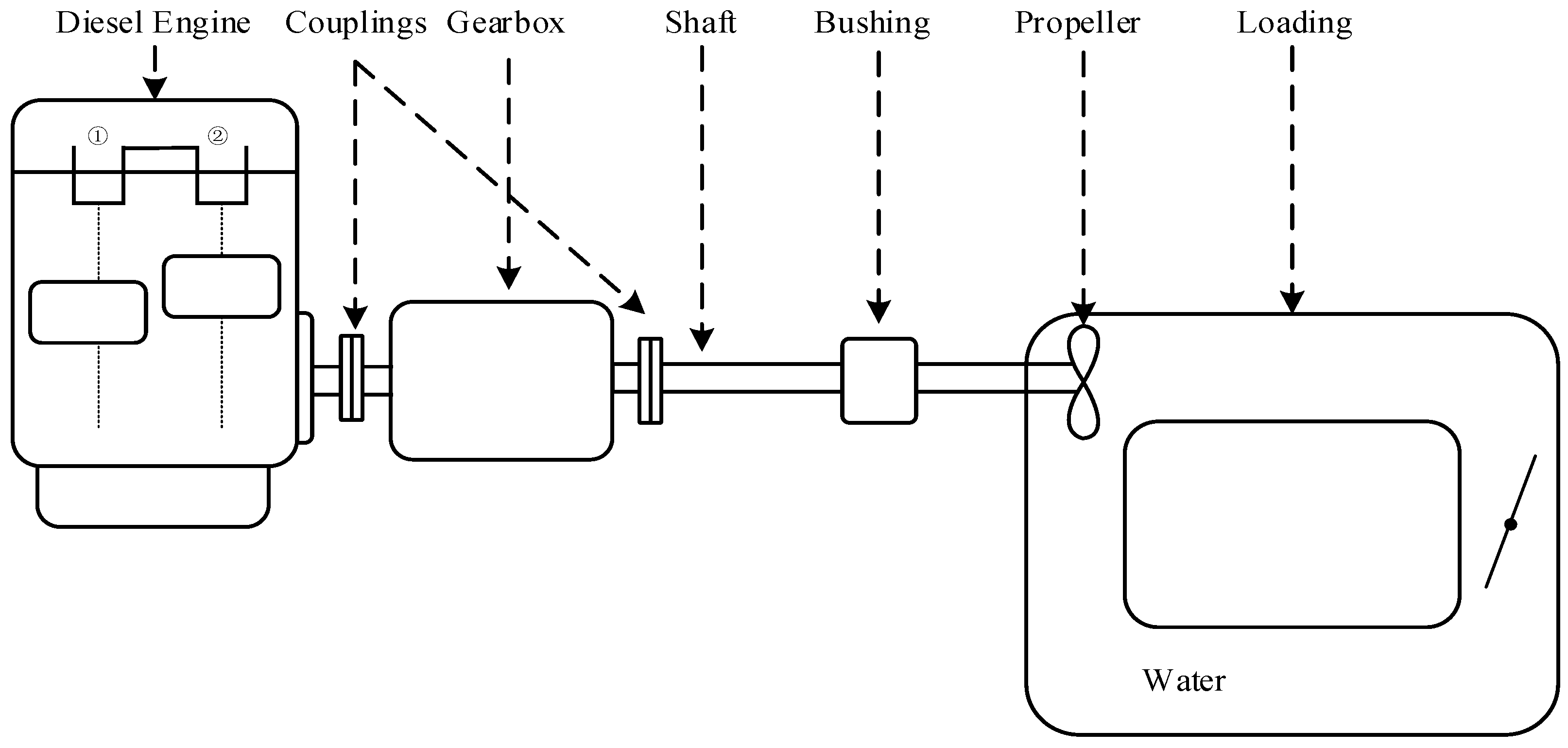
2.1. Marine System Simulator

A marine system simulator is designed in the laboratory for the investigation, which is shown in Figure 1. The test rig mainly consists of a two-cylinder diesel engine (Beta14), a gearbox (TMC40), a propeller, and a water tank. The Beta14 diesel engine is widely used in marine machinery and has a maximum power of 9.5 kW. Its specification is provided in

Table 1. Specification of Beta14 engine.

Specifications	Values
Model	Beta 14
Cylinder	2
Bore	67 mm
Stroke	68 mm
Displacement	479 cc
Combustion	Naturally aspirated, indirect injection
Power output	9.5 kW@3600 rpm
Maximum Torque	29.7 Nm@2600 rpm

. The mounting system is the original set from the manufacturer, and the installation requirements, including the angle, height, and positioning, were fully met. The frame used is rigid enough to have much higher natural frequencies than the mounting systems and engine operating speeds. The installation of the engine is well designed to simulate the real working conditions on a boat. We fully understand that the small marine engine used in the rig is different from the gigantic one. The deployment of the small marine engine is limited by lab space, risk and safety, funding, etc. The working principles of reciprocating diesel engines are the basis of the developed methods, which are transferable for monitoring large marine engines. The lubricant oil used for the engine is SAE 15 W/40. There are also circulations of freshwater and seawater for cooling purposes to simulate real marine working conditions. The engine is mounted on vibration absorber pension devices. A pair of spur pinions and gears in the gearbox transmit the torque from the clutch in the engine flywheel to the coupling. Then, the driving shaft drives the propeller immersed in water to rotate. To ensure the safe operation of the propeller, the tank is filled with water. There is a valve for adjusting the water circulation volume to simulate different load levels in the marine environment. The schematic diagram of the simulator is further demonstrated in Figure 2, which gives a clearer illustration of the configuration of the experiment setup. The rotating speed of the engine and the loading levels on the propeller are controlled by an integrated panel, which is located separately from the marine engine system simulator for safety. A dedicated in-house data acquisition software is being developed for the test, and the data collection strategy will be described next. The simulator can provide an essential platform for condition monitoring and fault diagnosis research, decreasing the costs and risks of direct field tests in the shipbuilding industry and for vessel owners.

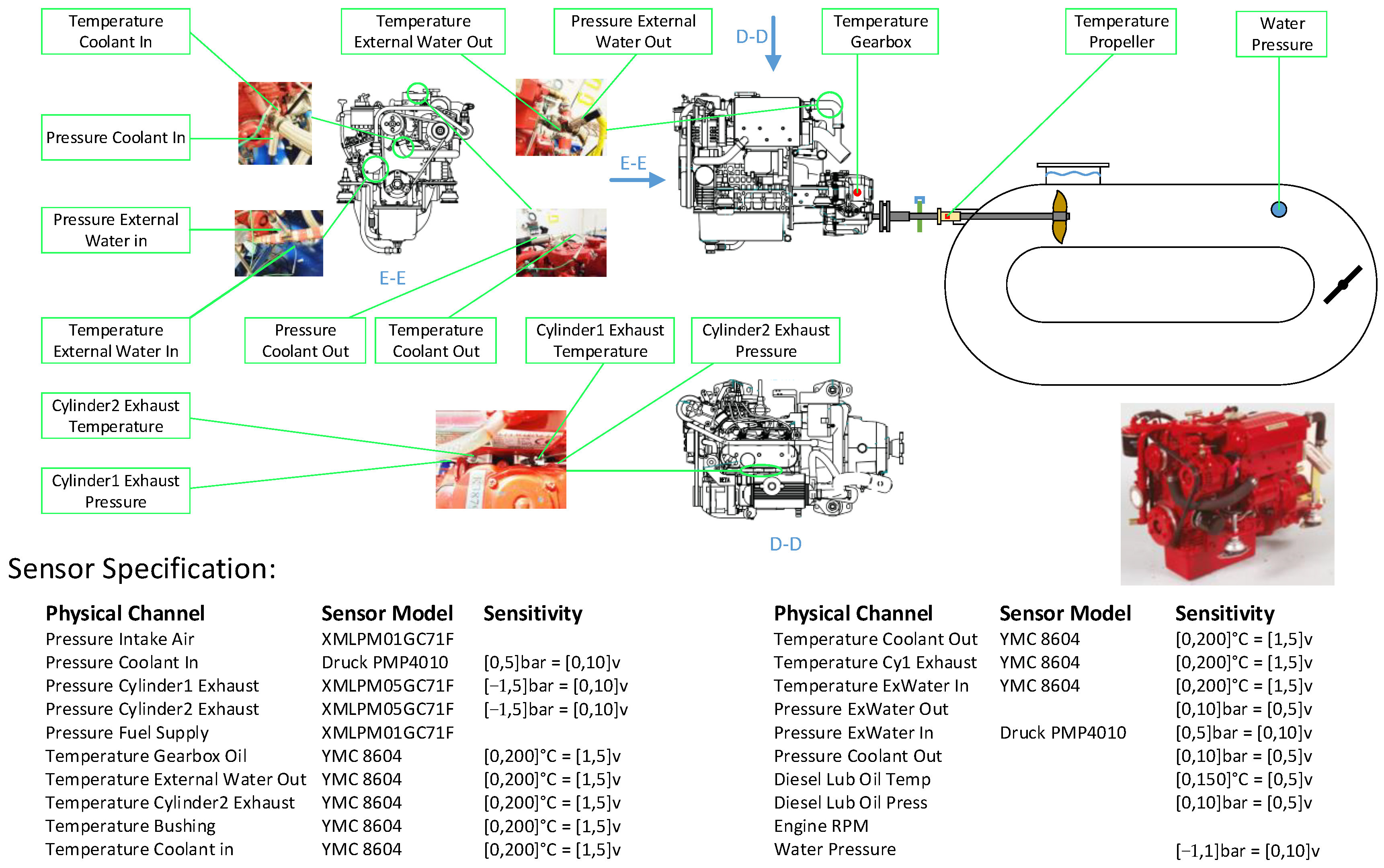
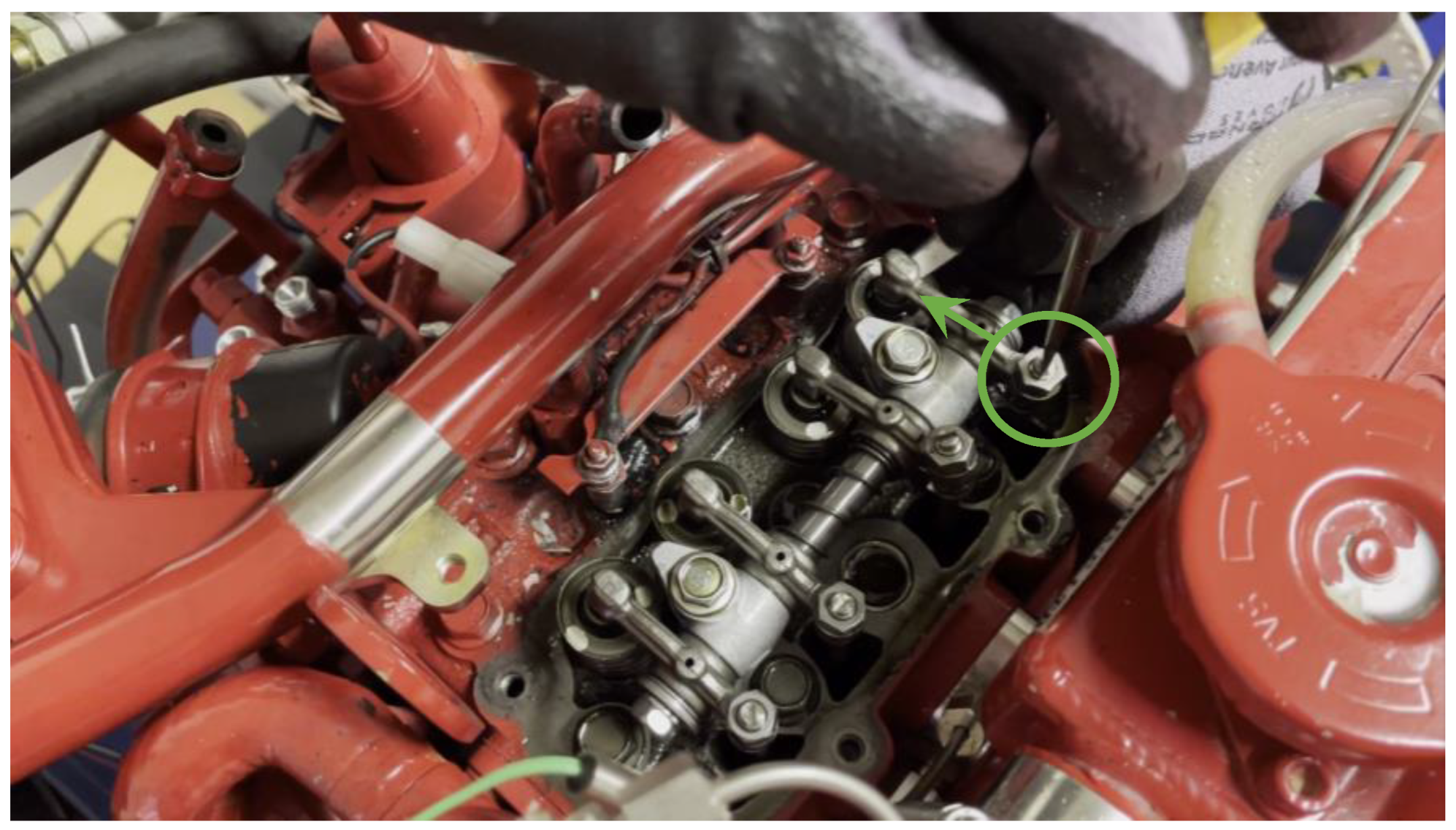
2.2. Sensor Placement

To facilitate the effective monitoring of all critical sub-systems in the marine power system, various sensors are placed to gather two types of data: static and dynamic. The static data specifically refers to the temperatures and pressures, which change slowly. The temperatures and pressures of the coolant, freshwater, seawater, cylinder exhaust gas, gearbox, and water in the tank are monitored. The sensors used and their sensitivities for static data collection are provided in Figure 3. For the static data, the sampling frequency is 1 Hz. Then, the static data will be transmitted by the CAN bus to a computer for further processing. Dynamic data represents the transiently changing sources, including TDC, IAS, and vibration signals. More specifically, the TDC and IAS of the engine, the IAS of the propeller, and the vibrations of the engine head, body, pump, gearbox, and propeller are monitored. The details of the transducer models used and their instalments are shown in Figure 4. In experimental tests, the static data is collected continuously, and the dynamic data is stored for 40 s every 3 min using a sampling frequency of 102.4 kHz. This high sampling frequency can ensure all the information in the dynamic data is preserved. Dynamic data is transmitted via the LAN cable to the connected computer. When novelties are detected based on the online CM method, an alarm will be sounded for the user’s attention. This strategy can save computation time and space for data storage while, in the meantime, being alerted. It should be noted that we previously mentioned that in-house data acquisition control software is used in our tests, and the above control parameters can be conveniently adjusted to meet different requirements.

3. Online Anomaly Detection

3.1. Processing of Data

For all collected static data, any extreme outlier data points will be filtered concerning the working conditions, i.e., the rotating speed of the engine and load levels. This is because the temperatures and pressures at a given working condition will change gradually from the perspective of a natural process. It also excludes any measurement errors that do not represent the real states. The engine torque overcomes the torque of the propeller, which is reflected by the water pressure in the tank where the propeller operates. We use the load level, i.e., the water pressure in the water tank as a condition parameter (the water pressure is measured in the water tank as marked in Figure 1) because the instantaneous torque generated by the engine is difficult to directly measure.

The dynamic data set collected in the test covers the instantaneous angular speeds (IAS) of the diesel engine and the propeller, as well as the vibrations of the engine head, engine body, pump, and journal bearing, as illustrated in the sensor placement shown in Figure 4. These channels measure the dynamic characteristics of the system at a very high sampling frequency. To effectively process the dynamic data, filtering and noise suppression are carried out. It enables accurate feature extraction and fault modelling. The opening and closing timing of intake and exhaust valves, as well as the combustion timing of the two-cylinder diesel engine, are analysed based on the working mechanisms, as shown in Figure 5. The two combustion actions in the two cylinders take place in the first cycle with a phase lag of 180°. In a complete working period, the intake and exhaust valves will open and close in the order given in Figure 5 to ensure the proper flow of air. The timing also provides useful hints for novelty detection.

The time-synchronous analysis (TSA) method and angular domain resampling (ADR) are used to process other vibration and IAS signals. The vibrations of the engine head are resampled in the angle domain. Moreover, a short-time Fourier transform (STFT) of the engine head vibration signal gives the instantaneous frequency map characteristics. The cylinder head vibrations are sensitive to the main impact events, for instance, combustion and valve landing. The opening of inlet and exhaust valves is relatively smooth and difficult to observe in certain health conditions. The low-frequency components are rich during the engine’s working cycle, which is induced by the engine’s rotation, air flow, and tribodynamics. The amplitude and timing of cylinder head vibrations are quite useful for engine health monitoring. Application of the envelope analysis to the engine head vibration data can help track the effects of combustion. The amplitudes caused by combustion in the two cylinders can provide useful information when there are anomalies. The analysis procedures discussed above are sequentially applied to other dynamic data channels, such as engine body vibrations, pump vibrations, journal bearing vibrations, and propeller IAS. These analysis results decrease the scale of data volumes and provide the basis for feature extractions that can be used for the online CM and FD of the marine engine system. For example, the encoder signal and engine IAS can be used for detecting misfire faults, incomplete combustion, and cylinder leakage faults. The fault location and severity can also be identified based on the timing and deviations of the features from baseline values. The engine head vibration signal provides features like combustion impact timing and amplitudes, valve landing impacts, and high-frequency RMS, which can be associated with injector and pump wear as well as valve leakage. The detailed monitoring and diagnosis rules and procedures will be elaborated in different fault simulations. The experimental rig is designed to measure multiple channel signals for comprehensive running condition detection and fault identification, although different types of faults are not necessarily present simultaneously in the marine engine system. More specifically, one can choose to plant a known fault to test the functionality of the CM system. However, a detection method is needed to enable efficient novelty monitoring after pre-processing and feature extraction from the static and dynamic data. In the rest of this section, a physics-based real-time CM modelling method for the marine power system will be established.

3.2. Physics-Based Multivariate Modelling

As explained previously, physics in such a marine engine system is important and any CM methods that do not rely on the physical working principles of the power system can produce results that are hard to interpret. The multivariate modelling is carried out based on the simplex-form polynomial formulation as

$$F\left(x_1,x_2,\cdots ,x_m\right)={\beta }_0+{\beta }_1{x}_1+{\beta }_2{x}_2+\cdots {+\beta }_{m+1}{x}_2+{\beta }_{m+2}{x}_1^2+{\beta }_{m+3}{x}_1{x}_2+\cdots ,$$

(1)

where m is the number of variables. In practice, only finite modelling order can be possible. After a re-arrangement, the compact form of an r-order multivariate model with the least number of terms can be given by

$$F(x_1,x_2,\cdots ,x_m)={\sum }_{0\le i_1+i_2+\cdots +i_m\le r}{\beta }_{i_1,i_{2,}\cdots ,i_m}{x}_1^{i_1}{x}_2^{i_2}\cdots x_m^{i_m},$$

(2)

where $i_1,i_2,\cdots ,i_m$ represent the indicators as well as the order of variables, ${\beta }_{i_1,i_{2,}\cdots ,i_m}$ is the unknown coefficient and $x_1,x_2,\cdots ,x_m$ denote the variables. Equation (2) can be further simplified as

$$F(x_1,x_2,\cdots ,x_m)={\mathit{\beta }}^T\mathit{X},$$

(3)

where

$$\mathit{\beta }=\left[{\beta }_{0,\cdots ,0},{\beta }_{\mathrm{1,0},\cdots ,0},{\cdots ,{\beta }_{0,\cdots ,\mathrm{0,1}},{\beta }_{\mathrm{2,0},\cdots ,0},\beta }_{\mathrm{1,1},0,\cdots ,0},\cdots ,{\beta }_{0,\cdots ,\mathrm{0,2}},\cdots ,{\beta }_{r,0,\cdots ,0},\cdots ,{\beta }_{0,\cdots ,0,r}\right],$$

(4)

$$\mathit{X}=\left[1,x_1,x_2,\cdots ,x_m,x_1^2,x_1{x}_2,\cdots ,x_m^2,\cdots ,x_1^r,\cdots ,x_m^r\right].$$

(5)

From Equations (4) and (5), it is easy to assign the powers of variables based on the subscript indices of the corresponding coefficients. The above formulation describes the inherent relationships between multiple variables. The running state of the marine power system being monitored is largely dependent on its working conditions. Therefore, the rotating speed and external load level (pressure in the water tank) are used as variables for other monitored static variables. For dynamic data, the RMS of the engine IAS for every data file stored in a specified time interval is used similarly to the engine RPM for static data. The averaged water load pressure in the tank for the same time interval is used for dynamic data. When the working condition variables themselves are to be modelled, the exhaust gas temperature or journal-bearing vibration features are used alternatively. Thus, complete relationships can be built. To obtain the unknown coefficients of the models for variables, baseline data is acquired using the healthy marine power system under different working conditions. Then, a fitting can be done to find the coefficients based on the fault-free datasets. When the models are fully established, they are used to monitor the condition of the power system by calculating the residuals between predicted data for variables using their models and measured data. The following residual for each monitored variable can be calculated:

$$\widehat{F_t}\left(x_1^{*}{,x}_2^{*},\cdots {,x}_m^{*}\right)={\mathit{\beta }}^T{\mathit{X}}^{*},$$

(6)

$$R\left(t\right)=t^{*}-\widehat{F_t},$$

(7)

where an asterisk means measured data, $\widehat{F_t}$ represents the predicted value obtained from the model of variable t, $R\left(t\right)$ is the residual between the predicted and measured values. Abnormally is deemed to happen if the residual is large, i.e.,

$$\left|R\left(t\right)\right|>\delta ,$$

(8)

where $\delta$ is a positive number generated by the prediction step, denoting the confidence level of the predicted value $\widehat{F_t}$. The above threshold criterion can also be expressed by

$$t^{*}>\widehat{F_t}\left(x_1^{*}{,x}_2^{*},\cdots {,x}_m^{*}\right)+\delta \mathrm{or}{t}^{*}<\widehat{F_t}\left(x_1^{*}{,x}_2^{*},\cdots {,x}_m^{*}\right)-\delta$$

(9)

Based on the above justification, any new data can be evaluated and the health state of the variable can be estimated. According to the physics of the system, a certain group of variables will indicate a specific fault in a subsystem, such as engines and bearings. Faults are identified and prompted when several data points exceed the limits to reduce false alarms.

4. Fault Simulations

In this section, two fault simulation experiments of the marine engine system are carried out, and the above method is applied to test its efficacy. For the baseline condition test, the working conditions are adjusted to cover more scenarios and ensure the physics-based models learn as much knowledge as possible about the engine system [25]. The rotating speed and load level evolutions are shown in Figure 6 and Figure 7. As can be seen from the two figures, different combinations of the two variables are included to simulate different working conditions. Next, three manually planted faults in the system are tested.

4.1. Misfire

A misfire fault is a common failure in internal combustion engines, and it leads to poor performance of the engine as well as degradation of other components. Spark failure, mixing issues of air and fuel, and incorrect valve timing are the main causes of the misfire fault. The pressure in cylinders can be used to monitor such faults, but it requires high-standard transducers, and their installation is a great challenge. Exhaust gas pressure and composition are also common indicators for diagnosing the misfire fault. However, its accuracy cannot be guaranteed in the complex working environment a marine engine is working in, and it needs additional gas composition analyzers. According to the physics behind the engine, the temperature of a misfired cylinder will decrease significantly. Due to the misfire in a cylinder, the IAS peak of the faulted cylinder will show prominent decreases due to the absent work the cylinder is normally doing. In fault simulation, the fuel from Cylinder 1 is redirected to a spare vessel, as shown in Figure 8. Thus, no fuel is injected into the faulted cylinder, and it cannot properly combust. In such a way, the misfire effects are simulated in the diesel engine.

The collected data for the misfire fault is sent to the CM model for novelty detection. Although many physical parameters are monitored, only the variables associated with the fault are analysed and presented. Others are normal within the model-predicted confidence interval. Figure 9 shows the healthy data and fault data for static variables, i.e., the exhaust gas temperatures, and Figure 10 demonstrates the trends for dynamic features, i.e., engine head vibration TSA peak values for combustions.

The baseline modelling for both static and dynamic data and its 99% confidence interval show excellent wrapping of most of the healthy data. As can be seen from Figure 9, the most direct indicator is demonstrated by the significant decrease in the exhaust gas temperature of the misfired cylinder 1, dropping from its predicted interval to 70–80 °C. This is natural since there is no combustion in the cylinder and the exhaust gas temperature is low. In the test, the rotating speed (around 1200 rpm) and load level (around 0.19 bar) are controlled to be the same as in healthy status. Thus, more work is done by Cylinder 2, and its exhaust gas temperature is higher than predicted. The engine head vibration signal is processed by the TSA technique to extract the amplitudes at the combustion timing of the two cylinders. Similar to the exhaust gas temperature, the vibration peak values corresponding to the combustion of Cylinder 1 are significantly lower than the model-predicted band, while those for Cylinder 2 combustion are approaching their upper limits, as shown in Figure 10. To further look into the physics, Figure 11 shows the engine IAS fluctuations with its mean component removed, which clearly indicates the effects of working strokes in cylinders. It is evidently shown that the impulse for cylinder 1 is reduced while the peak and its following part are higher than in healthy conditions. The reason why the impulse after the first peak is higher than normal is that the rotating speed is kept nearly the same for both states, and more work is done by the other cylinder when one cylinder misfires. The above characteristics can detect the misfire fault in the system and identify which cylinder is faulted.

4.2. Exhaust Valve Leakage

Exhaust and inlet valves often work in high-pressure and high-temperature environments. The frequent open and close operations cause the valves to wear and loosen, leading to leakage. The output power of the engine will be decreased due to this fault, which can pollute the environment. Although the fault can lead to a series of phenomena, the engine head vibration can be more robustly diagnosed. The vibration signals of the engine head are periodic due to the working cycles and non-stationary as well. Accurate monitoring of it can be difficult in engineering. However, the vibrational features associated with valve leakage are often exhibited in the high-frequency domain. Thus, it is feasible to identify the valve leakage fault by monitoring the vibrations of the engine head. In the simulation, the engine head is first removed. Then, the clearance of the exhaust valve is adjusted manually, as shown in Figure 12. After the adjustment, the engine head is reinstalled. The above modification produces a larger value of the clearance, which creates airflow through the valve and simulates the exhaust valve leakage issue in marine power systems.

Based on the physics and valve timing of the diesel engine, the main bearing impact RMS of the engine body vibrations and the TSA features of the engine head vibrations, including the high-frequency RMS associated with the inlet and exhaust actions and the valve impact RMS of the inlet and exhaust valves for both cylinders, are used to monitor the exhaust valve leakage fault. The leakage fault is implemented on the exhaust valve of Cylinder 2, as demonstrated in Figure 12. According to the test data and model predictions, the results for the high-frequency RMS of the engine head vibration signals are illustrated in Figure 13. The trends of the impact RMS caused by the inlet and exhaust valve landings for cylinders are depicted in Figure 14. Figure 15 shows the main bearing impact RMS results extracted from the TSA of the engine body vibration signals.

It can be seen from Figure 13 that the high-frequency RMS of the engine head vibration signals is significantly higher than the model-predicted confidence interval, indicating its abnormality. The valve landing RMS features in Figure 14 illustrate that those of the inlet valves for both cylinders are normal. The exhaust valve landing RMS for Cylinder 1 falls into the confidence interval, while that of Cylinder 2 exceeds the upper limit of predicted values. This is natural since the fault is pre-planted on the exhaust valve of Cylinder 2, and the results prove the ability of the model to identify the fault position. In setting the fault, the clearance value of the valve is adjusted to be larger than normal. Thus, the valve landing RMS of the engine head vibrations will increase. Similar characteristics are also found in the main bearing impact RMS of the engine body vibrations, as evidenced in Figure 15, where the deviation is more striking from the perspective of net magnitudes. The results validate the proposed model for diagnosing valve leakage faults.

5. Conclusions

In the present work, a marine system simulator is established, and a physics-based multivariate modelling method is proposed for the condition monitoring of the system. Measurements of many static and dynamic variables in the marine system, such as temperatures, pressures, and vibrations, are implemented. Data processing is described in detail, and the modelling theory is elaborated. The misfire of a cylinder and leakage of an exhaust valve are simulated in the test rig to test the validity of the proposed novelty detection method. In the misfire simulations, the temperature of the misfired cylinder exhaust gas is 30 °C lower than the estimated 99% confidence interval lower limit, while the engine head vibration TSA peak dropped from over 1000 m/s² to just a little above 200 m/s². For the exhaust valve leakage fault, the engine body vibration main bearing impact RMS associated with the leaked valve is almost 10 times the predicted values. These results show that the two faults are successfully diagnosed, and their positions are identified, indicating that the proposed physics-based approach is suitable for the condition monitoring of the power system. The findings reported could guide the engineers in efficient condition monitoring of such systems and aid in determining when the best time is to arrange maintenance. It is worth mentioning that more comprehensive fault simulations in different parts of the system will be carried out on the test rig for a broadened understanding of marine power systems. The CM method and measurement configuration can be integrated as a test system, which will be applied to onboard machines.

References

1. Xu, X.; Yan, X.; Yang, K.; Zhao, J.; Sheng, C.; Yuan, C. Review of condition monitoring and fault diagnosis for marine power systems. Transp. Saf. Environ. 2021, 3, 85–102. [Google Scholar] [CrossRef]
2. Zhang, H.; Li, Z.; Chen, Z. Application of grey modeling method to fitting and forecasting wear trend of marine diesel engines. Tribol. Int. 2003, 36, 753–756. [Google Scholar] [CrossRef]
3. Nejad, A.R.; Purcell, E.; Valavi, M.; Hudak, R.; Lehmann, B.; Gutiérrez Guzmán, F.; Behrendt, F.; Bõhm, A.M.; von Bock und Polach, F.; Nickerson, B.M. Condition monitoring of ship propulsion systems: State-of-the-art, development trend and role of digital Twin. In Proceedings of the ASME 40th International Conference on Offshore Mechanics and Arctic Engineering, Virtual, 21–30 June 2021; p. V007T007A005. [Google Scholar]
4. Byun, S.; Papaelias, M.; Márquez, F.P.G.; Lee, D. Fault-tree-analysis-based health monitoring for autonomous underwater vehicle. J. Mar. Sci. Eng. 2022, 10, 1855. [Google Scholar] [CrossRef]
5. Zhang, Y.; Hong, J.; Shi, H.; Xie, Y.; Zhang, H.; Zhang, S.; Li, W.; Chen, H. Magnetic plug sensor with bridge nonlinear correction circuit for oil condition monitoring of marine machinery. J. Mar. Sci. Eng. 2022, 10, 1883. [Google Scholar] [CrossRef]
6. Liang, X.; Fu, C.; Sun, X.; Duan, F.; Mba, D.; Gu, F.; Ball, A.D. An investigation of unsupervised data-driven models for internal combustion engine condition monitoring. In Mechanisms and Machine Science, Proceedings of the IncoME-VI and TEPEN 2021: Performance Engineering and Maintenance Engineering, Tianjin, China, 20–23 October 2021; Zhang, H., Feng, G., Wang, H., Gu, F., Sinha, J.K., Eds.; Springer: Cham, Switzerland, 2022; pp. 463–475. [Google Scholar]
7. Ma, J.; Fu, C.; Zhang, H.; Chu, F.; Shi, Z.; Gu, F.; Ball, A.D. Modelling non-Gaussian surfaces and misalignment for condition monitoring of journal bearings. Measurement 2021, 174, 108983. [Google Scholar] [CrossRef]
8. Jiang, J.; Hu, Y.; Fang, Y.; Li, F. Application and prospects of intelligent fault diagnosis technology for marine power system. Chin. J. Ship Res. 2020, 15, 56–67. [Google Scholar]
9. Vanem, E.; Storvik, G.O. Anomaly detection using dynamical linear models and sequential testing on a marine engine system. In Proceedings of the Annual Conference of the PHM Society, St. Petersburg, FL, USA, 2–5 October 2017. [Google Scholar]
10. Wang, J.; Zhang, C.; Ma, X.; Wang, Z.; Xu, Y.; Cattley, R. A multivariate statistics-based approach for detecting diesel engine faults with weak signatures. Energies 2020, 13, 873. [Google Scholar] [CrossRef] [Green Version]
11. Xu, Y.; Huang, B.; Yun, Y.; Cattley, R.; Gu, F.; Ball, A.D. Model based IAS analysis for fault detection and diagnosis of IC engine powertrains. Energies 2020, 13, 565. [Google Scholar] [CrossRef] [Green Version]
12. Perera, L.P.; Mo, B. Data analysis on marine engine operating regions in relation to ship navigation. Ocean Eng. 2016, 128, 163–172. [Google Scholar] [CrossRef]
13. Cao, W.; Dong, G.; Chen, W.; Wu, J.; Xie, Y. Multisensor information integration for online wear condition monitoring of diesel engines. Tribol. Int. 2015, 82, 68–77. [Google Scholar] [CrossRef]
14. Schneider, T.; Kruse, T.; Kuester, B.; Stonis, M.; Overmeyer, L. Evaluation of an energy self-sufficient sensor for monitoring marine gearboxes. Procedia Manuf. 2018, 24, 135–140. [Google Scholar] [CrossRef]
15. Fan, L.; Wen, L.; Bai, Y.; Lan, Q.; Xu, J.; Gu, Y. Research on the correlation between fuel injection quantity and key structural parameters for the fuel system of marine diesel engines. Proc. Inst. Mech. Eng. Part C J. Mech. Eng. Sci. 2021, 235, 7385–7398. [Google Scholar] [CrossRef]
16. Boullosa-Falces, D.; Barrena, J.L.L.; Lopez-Arraiza, A.; Menendez, J.; Solaetxe, M.A.G. Monitoring of fuel oil process of marine diesel engine. Appl. Therm. Eng. 2017, 127, 517–526. [Google Scholar] [CrossRef]
17. Johansen, S.S.; Nejad, A.R. On digital twin condition monitoring approach for drivetrains in marine applications. In Proceedings of the ASME 2019 38th International Conference on Ocean, Offshore and Arctic Engineering, Glasgow, Scotland, 9–14 June 2019. [Google Scholar]
18. Delvecchio, S.; Bonfiglio, P.; Pompoli, F. Vibro-acoustic condition monitoring of Internal Combustion Engines: A critical review of existing techniques. Mech. Syst. Signal Process. 2018, 99, 661–683. [Google Scholar] [CrossRef]
19. Fu, C.; Sinou, J.-J.; Zhu, W.; Lu, K.; Yang, Y. A state-of-the-art review on uncertainty analysis of rotor systems. Mech. Syst. Signal Process. 2023, 183, 109619. [Google Scholar] [CrossRef]
20. Dikis, K.; Lazakis, I.; Turan, O. Probabilistic risk assessment of condition monitoring of marine diesel engines. In Proceedings of the International Conference on Maritime Technology, Glasgow, Scotland, 7–9 July 2014. [Google Scholar]
21. Wang, R.; Chen, H.; Guan, C. A Bayesian inference-based approach for performance prognostics towards uncertainty quantification and its applications on the marine diesel engine. ISA Trans. 2021, 118, 159–173. [Google Scholar] [CrossRef] [PubMed]
22. Asuquo, M.P.; Wang, J.; Phylip-Jones, G.; Riahi, R. Condition monitoring of marine and offshore machinery using evidential reasoning techniques. J. Mar. Eng. Technol. 2021, 20, 93–124. [Google Scholar] [CrossRef]
23. Yan, X.; Sheng, C.; Zhao, J.; Yang, K.; Li, Z. Study of on-line condition monitoring and fault feature extraction for marine diesel engines based on tribological information. Proc. Inst. Mech. Eng. Part O J. Risk Reliab. 2015, 229, 291–300. [Google Scholar] [CrossRef]
24. Cai, C.; Weng, X.; Zhang, C. A novel approach for marine diesel engine fault diagnosis. Clust. Comput. 2017, 20, 1691–1702. [Google Scholar] [CrossRef]
25. Wang, J.; Sun, X.; Zhang, C.; Ma, X. An integrated methodology for system-level early fault detection and isolation. Expert Syst. Appl. 2022, 201, 117080. [Google Scholar] [CrossRef]
Figure 1. Marine system simulator.
Jmse 11 01241 g001
Figure 2. Schematic diagram of the experimental setup.
Jmse 11 01241 g002
Figure 3. Sensor placement for static data.
Jmse 11 01241 g003
Figure 4. Sensor placement for dynamic data.
Jmse 11 01241 g004
Figure 5. Timing for valves and combustion (IVC-intake valve closing, IVO-intake valve opening, EVC-exhaust valve closing and EVO-exhaust valve opening; ☆-combustion).
Jmse 11 01241 g005
Figure 6. Engine rotating speed for baseline data.
Jmse 11 01241 g006
Figure 7. Load levels for baseline data.
Jmse 11 01241 g007
Figure 8. Misfire fault simulation.
Jmse 11 01241 g008
Figure 9. Exhaust gas temperature for cylinders under healthy state and misfire of cylinder 1: solid lines-measured data, dashed lines-99% confidence interval predicted by the multivariate model. (C1 = Cylinder 1; C2 = Cylinder 2).
Jmse 11 01241 g009
Figure 10. Comparisons of engine cylinder head vibration TSA signal peak values under healthy conditions (solid lines-measured data, dashed lines-99% confidence interval predicted by the multivariate model): (a) C1, (c) C2 and faulty conditions, with misfire of cylinder 1: (b) C1 and (d) C2. (C1 = Cylinder 1; C2 = Cylinder 2).
Jmse 11 01241 g010
Figure 11. Engine IAS fluctuation comparisons for healthy state and misfire fault.
Jmse 11 01241 g011
Figure 12. Exhaust valve leakage simulation.
Jmse 11 01241 g012
Figure 13. Engine head vibration high-frequency RMS under healthy state and valve leakage: solid lines-measured data, dashed lines-predicted 99% confidence interval.
Jmse 11 01241 g013
Figure 14. Engine head vibration valves landing RMS under healthy state and valve leakage: solid lines-measured data, dashed lines—predicted 99% confidence interval.
Jmse 11 01241 g014
Figure 15. Engine body vibration main bearing impact RMS under healthy state and valve leakage: solid lines-measured data, dashed lines—predicted 99% confidence interval.
Jmse 11 01241 g015