Evolution Wave Condition Using WAVEWATCH III for Island Sheltered Area in the South China Sea

Abstract

Wave conditions around islands in the South China Sea (SCS) are of significant interest due to their importance for marine operations and coastal engineering. Understanding and accurately predicting wave characteristics in this region are crucial. In this study, the third-generation wave model WAVEWATCH III is employed to examine wave conditions around islands in the SCS. According to the water depth and significant wave height, the sea state around the island was classified into two categories: typhoon sea state and moderate sea state. Several popular wind input–dissipation source terms (ST2, ST4 and ST6) are used to assess the typhoon sea state and the moderate sea state separately. The results are validated by field wave data. ST4 and ST6 show good performance in significant wave height for moderate sea states, while ST2 is good at the mean wave period. For the typhoon sea state, ST2 gives the best results in significant wave height with larger correlation coefficients and a smaller RMSE. The above results provide valuable insights into the effects of different source terms on the accuracy of wave simulations for different sea states. The spatial distribution of the significant wave heights is also demonstrated with ST2, which may be useful for assessing the wave conditions of marine structures from the large scale of the SCS to the island scale of the Yongle Atoll.

1. Introduction

Wave conditions are very important for the safety of marine structures. The accurate assessment of wave conditions can optimize the design parameters and enhance the performance of marine structures [1]. Marine structures, such as very large floating structures, fish farming cages and plate forms, are very important for island development, especially in remote areas away from the mainland, providing spaces for living and production. However, the wave conditions around islands and reefs are highly dependent on the complex submarine topography. Due to the specific bathymetry around islands in the South China Sea, the physical processes involved in wave evolution are different between deep-sea areas and island areas. Therefore, the use of the WWIII model has been extended from deep-sea and continental shelf areas to shallow-water nearshore areas. The applicability of the WWIII model in near-island areas has been extensively verified [2,3,4,5]. Moreover, several studies have confirmed that the WWIII model provides generally good results at different wind forces in deep water by comparing it with other models such as SWAN, WAM, WAVAD and WWIII [6,7,8,9].

The WWIII model offers a diverse range of source terms, particularly for wind input–dissipation, and scholars have conducted numerous studies to determine their applicability and accuracy [10,11,12]. These include the WAM Cycle 3 (ST1) package [13,14], the Tolman and Chalikov (1996) package [15] (ST2), the WAM Cycle 4 (ST3) package [16,17], the Ardhuin et al. (2010) package [18] (ST4), and the Zieger et al. (2015) [19] source term (ST6). Several scholars have examined the performance of different wind input–dissipation source terms in different regions of the globe under different wind forces. By comparing the performance of ST2, ST3, ST4 and ST6, Liu et al. [20] found that ST2 was the least accurate formula for simulating Hurricane Ivan, while ST4 results were in better agreement with the measurements. The same hurricane simulation results [21] show that the most appropriate formula is not the same for different areas (Gulf of Mexico). For the northern Tyrrhenian Sea and off the Mediterranean Spanish coast, Mentaschi et al. [22] showed that the source term introduced by ST4 is the best overall choice. However, Kalantzi et al. [23] found that neither ST1 nor ST2 can properly simulate waves in the presence of swells. Foli et al. [24] demonstrated that ST2STAB (a variant of ST2) and ST6 were suitable for simulating wave height and direction, respectively, in the entire West African region. In particular, the ST2 has gained wide acceptance in typhoons and rough sea conditions [25,26,27,28,29].

In general, waves passing around islands will experience refraction, diffraction, and deformation [30,31]. Moreover, the South China Sea (SCS) is known to have abundant marine resources, particularly in the vicinity of reef islands [32,33]. The measurement location in our research has a depth of 30 m. Due to the significant differences in wave conditions, we have categorized them into a moderate sea state and a typhoon sea state based on the characteristic wave length. In the following sections, we aim to present a representative wave forecasting scheme for the Yongle Atoll area under different oceanic conditions, namely, the typhoon sea state and moderate sea state. Section 2 describes the study area, data and wave model. The numerical wave conditions are validated using field wave data, and the best parameter choices and plan are selected for the moderate sea state and the typhoon sea state in Section 3. Conclusions are given in Section 4.

2. Methods and Data

2.1. Study Area

Yongle Atoll, located in the northern part of the SCS (Figure 1), is vulnerable to frequent typhoons in the western Pacific Ocean. Due to the complex and variable seafloor topography around the islands and reefs, establishing an accurate numerical model for the Yongle Atoll is of great importance. Therefore, this study covers the entire marine environment of the SCS (longitudes 104–118° E; latitudes 12–24° N), including the Yongle Atoll area (longitudes 111.49–111.805° E; latitudes 16.4198–16.6180° N).

2.2. Spectral Balancing Equation

Third-generation wave models, such as WAVEWATCH III, are based on the wave spectrum balance equation and widely applied in both theoretical and practical applications [34]. In general, WWIII simulates the propagation of waves by solving the wave action balance equation:

$$\frac{D\left(N\left(k,\theta ;x,t\right)\right)}{Dt}=\frac{S\left(\mathrm{k},\theta ;x,t\right)}{\sigma }$$

(1)

$$N\left(k,\theta ;x,t\right)=\frac{F\left(k,\theta ;x,t\right)}{\sigma }$$

(2)

where $F$ is the fundamental spectrum; $N$ is the wave action density spectrum; $S$ represents the net effect of sources and sinks for the spectrum $F$. $k$, $\theta$, and $\sigma$ represent the wavenumber, wave direction, and intrinsic frequency, respectively, and $x$ and $t$ are variables that represent space and time [35]. Then, the balance Equation (1) is extended to the following conservative form:

$$\frac{\partial N}{\partial t}+{\nabla }_x\cdot \dot{x}N+\frac{\partial }{\partial k}\dot{k}N+\frac{\partial }{\partial \theta }\dot{\theta }N=\frac{S}{\sigma }$$

(3)

$$\dot{x}=c_g+U$$

(4)

$$\dot{k}=-\frac{\partial \sigma }{\partial d}\frac{\partial d}{\partial s}-k\cdot \frac{\partial U}{\partial s}$$

(5)

$$\dot{\theta }=-\frac{1}{k}\left[\frac{\partial \sigma }{\partial d}\frac{\partial d}{\partial m}+k\cdot \frac{\partial U}{\partial m}\right]$$

(6)

where $c_g=(c_g\sin \theta ,c_g\cos \theta )$ denotes the group velocity; $d$ is the mean water depth; and $U$ is the current velocity (depth- and time-averaged over the scales of individual waves). $S$ is a coordinate in the direction $\theta$, and $m$ is a coordinate perpendicular to $S$. Equation (3) is used for Cartesian coordinates. For large-scale calculations, this equation is usually applied to spherical coordinates, defined by longitude $\lambda$ and latitude $\varphi$ [36].

$$\frac{\partial N}{\partial t}+\frac{1}{\cos \varphi }\frac{\partial }{\partial \varphi }\dot{\varphi }N\cos \theta +\frac{\partial }{\partial \lambda }\dot{\lambda }N+\frac{\partial }{\partial k}\dot{k}N+\frac{\partial }{\partial \theta }{\dot{\theta }}_{g}N=\frac{S}{\sigma }$$

(7)

$$\dot{\varphi }=\frac{c_g\cos \theta +U_{\varphi }}{R}$$

(8)

$$\dot{\lambda }=\frac{c_g\sin \theta +U_{\lambda }}{R\cos \varphi }$$

(9)

$${\dot{\theta }}_g=\dot{\theta }-\frac{c_g\tan \varphi \cos \theta }{R}$$

(10)

where $R$ is the radius of the earth, and $U_{\varphi }$, and $U_{\lambda }$ are current components. $\theta =0$ corresponds to waves traveling from west to east.

In WWIII wave models, energy is conserved in the absence of currents. However, when currents are present, the energy of the spectrum is no longer conserved because the currents shift the average momentum acting on the waves [37,38]. Therefore, the wave action density spectrum is the preferred choice in the WWIII model.

The net source term $S$ in fact consists of four main components: an atmosphere–wave interaction term $S_{in}$, a nonlinear wave–wave interaction term $S_{nl}$, the dissipation term $S_{ds}$, and the wave–bottom interaction term $S_{bot}$. However, in this study, we need to consider the effect of shallow water on wave evolution around the Yongle Atoll. Specifically, depth-induced breaking ($S_{db}$) is crucial for numerical simulations in shallow water. To provide a more realistic initial wave growth, a linear input term $S_{ln}$ can also be added. In summary, the main source terms considered in the calculation process are presented in the following equation [26,39]:

$$S=S_{ln}+S_{in}+S_{nl}+S_{ds}+S_{bot}+S_{db}$$

(11)

2.3. Spatial Grids

To balance computational efficiency with accuracy, an unstructured triangular grid consisting of 42,445 nodes and 84,961 cells was selected for our calculations, as shown in Figure 2 [40]. Although our primary focus is on the Yongle Atoll area in the SCS, this grid covers the entire expansive computational domain of the SCS. To ensure computational efficiency, a coarser grid is utilized outside of the Yongle Atoll. The grid resolution becomes progressively finer closer to the Yongle Atoll, enhancing the accuracy of our calculations.

2.4. Wave Model Setup

The study utilized WAVEWATCH III version 5.16 to investigate the wind input–dissipation source terms for ocean wave simulations. The code for different source items is modular, providing multiple options for the same source term [41]. Wind input term $S_{in}$ and dissipation terms $S_{ds}$ are two different processes, but the balance of these two source terms determines the overall growth characteristics of wave energy and is considered interrelated. In this study, we focus on the effect of different input–dissipation source term packages, which are listed below.

• Tolman and Chalikov 1996 (ST2) package [15,42,43,44];
• Ardhuin et al. 2021 (ST4) package [18,45];
• Zieger et al. 2015 (ST6) package [19].

The wave energy balance equation [39] is solved using the same source terms as described in

Table 1. Source terms switches deployed in the WWIII model in this study.

Source Term	Switch	Description
Linear input term	LN1	Cavaleri and Malanotte-Rizzoli 1981 [46]
Nonlinear interactions	NL1	Discrete interaction approximation [47]
Wave–bottom interaction	BT1	JONSWAP bottom friction [36,48,49]
Wave breaking	DB1	Battjes and Janssen 1978 [50]
Wind input–dissipation term	ST2/ST4/ST6	Tolman and Chalikov 1996/Ardhuin et al. 2010/Zieger et al. 2015 [18,19]

. The spectrum is discretized using 30 frequencies ranging from 0.04118 to 0.6532 Hz with an increment factor of 1.1 and 36 directions with a 10-degree directional increment. To improve computational efficiency, WWIII utilizes four types of time steps: a maximum global time step and a maximum CFL time step for x-y of 20 s; a minimum source term time step of 20 s; and a maximum CFL time step for x-y of 10 s. Other parameter schemes remain the same as the default values of the WWIII model, and more details can be found in the user manual [35].

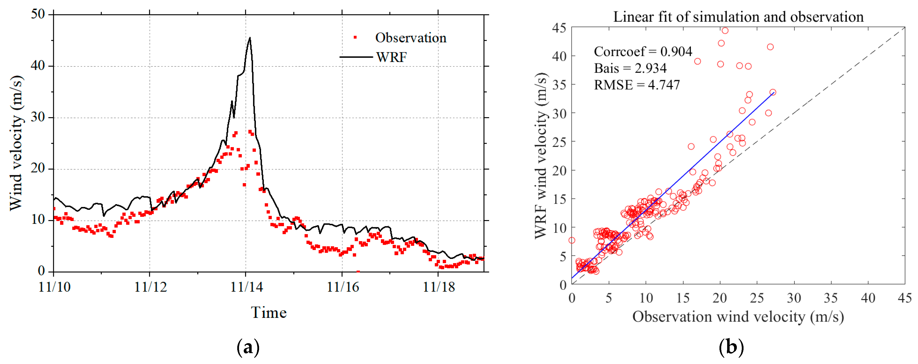
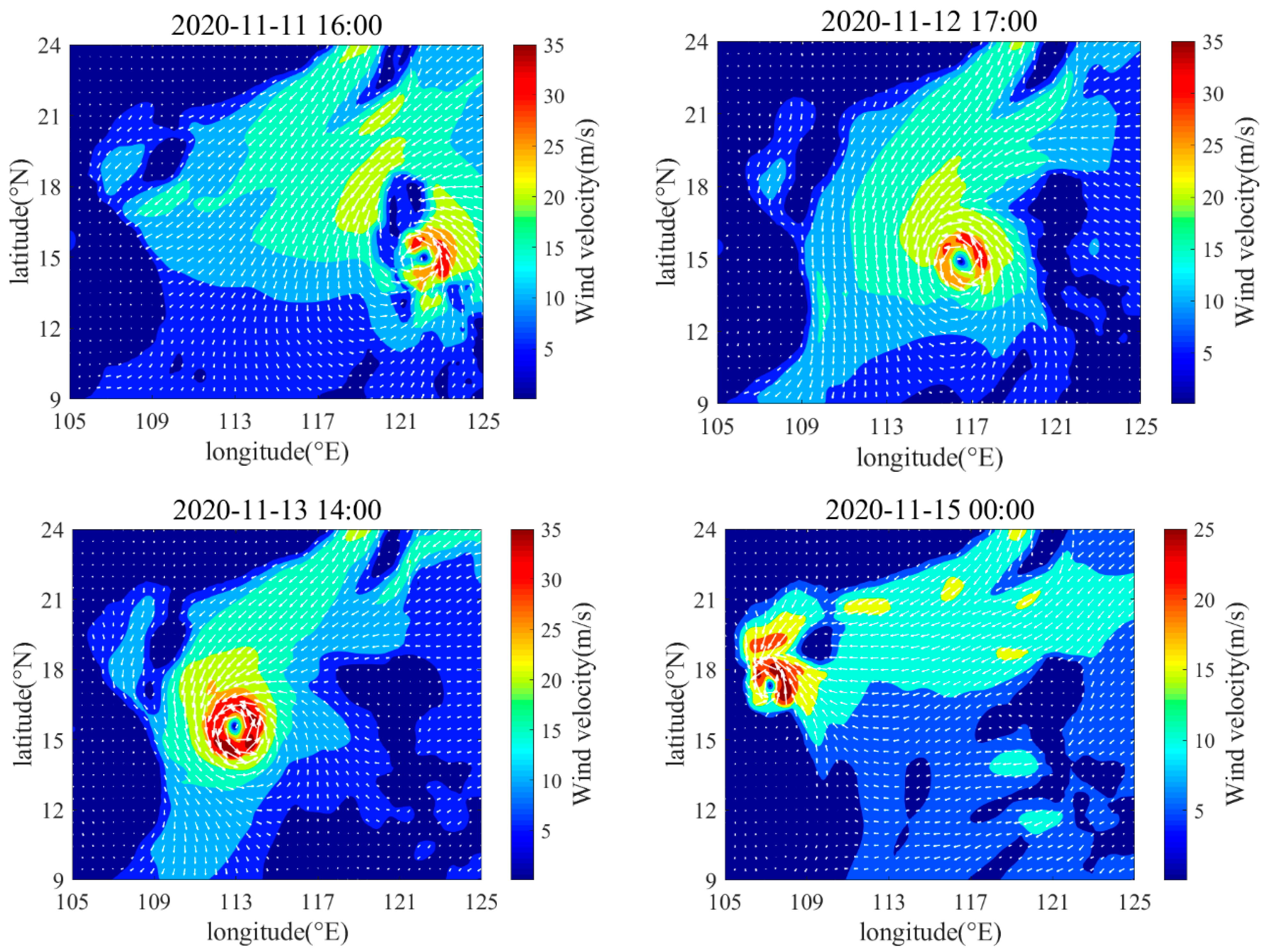
2.5. Wind Field Data

This study employs the Weather Research and Forecasting (WRF) model to perform reanalysis of wind fields. The wind field was forced with 1 h time step WRF from reanalysis dataset, with a spatial resolution of 0.1° in both longitude and latitude, and the number of grids is 201 and 151, respectively. Various studies [39,51,52,53] have shown that the accuracy of the wind field has a significant impact on the wave field. In order to verify the accuracy of the wind field, the correlation coefficient (Corrcoef), root mean square error (RMSE) and bias (Bias) are introduced in this paper to describe the relationship between the measured and simulated values. These statistics are defined by the following equations:

$$\mathrm{corrcoef}=\frac{{{\displaystyle \sum }}_{i=1}^N\left(x_i-\overline{x}\right)\left(y_i-\overline{y}\right)}{\sqrt{\left[{{\displaystyle \sum }}_{i=1}^N{\left(x_i-\overline{x}\right)}^2\right]\left[{{\displaystyle \sum }}_{i=1}^N{\left(y_i-\overline{y}\right)}^2\right]}}$$

(12)

$$RMSE=\sqrt{\frac{1}{N}{\displaystyle \sum }_{i=1}^N{\left(y_i-x_i\right)}^2}$$

(13)

$$\mathrm{Bias}=\overline{y}-\overline{x}$$

(14)

where $x_i$ and $y_i$ represent the measured and simulated values, respectively, and $N$ is the number of samples. The wind velocity simulation and observation comparison are presented in Figure 3. The results show a high correlation coefficient of 0.905, indicating good agreement. However, the simulated wind velocity is slightly higher than the measured wind velocity, with a bias of 1.233. Based on these results, the simulated wind field is suitable for use as input data for the calculation model.

2.6. Sea Condition

Moderate sea state is defined as SWH less than one meter in this paper, while severe wave condition, referred to as typhoon sea state, corresponds to SWH larger than one meter at Yongle Atoll. It should be noted that for the most common wave steepness of 1:30, one meter SWH corresponds to a wave length of 30 m, which is the wave depth of the measurement points as shown in Figure 4. Notably, the water depth of both points (Point 1 and Point 2) is 30 m.

The typhoon sea conditions in this article calculate the wave evolution from 3 September to 15 September 2020, during which the wind level in the target sea remains within level 5 (i.e., wind speed below 10.7 m/s), and the sea state is categorized as level 4.

The typhoon sea conditions in this article focus specifically on Typhoon No. 22 of 2020, known as “Vamco”. “Vamco” originated in the sea east of the Philippines on 9 No-vember 2020 and reached the eastern part of the SCS on 12 November. The path of the typhoon propagation from southeast to northwest is depicted in Figure 5.

To gain a clearer understanding of the wind velocity during the movement of the ty-phoon, Figure 6 displays the comparison between the measured and simulated wind velocity for “Vamco”. It is evident that the simulated wind velocity is considerably higher than the measured wind velocity near the peak of the typhoon, with the simulated values being about 1.8 times greater than the measured values. The velocity vectors of the typhoon’s passage are shown in Figure 7.

3. Results and Discussions

3.1. Moderate Sea State Wave Hindcasts

3.1.1. Significant Wave Height (SWH)

During the moderate sea state, the SWHs at both point 1 and 2 did not exceed 1 m and showed fluctuations in response to changes in wind velocity. A comparison of the time history curves between the simulated SWHs and the measured values revealed the performance of the different input–dissipation source term schemes in Figure 8. All three input–dissipation source term schemes were able to adequately capture the trend of the SWHs in the moderate sea state. However, the SWHs simulated by the ST2 scheme were consistently larger than the measured values, especially after 8 September 2020. This suggests that the ST2 scheme dissipates energy more slowly than the ST4 and ST6 schemes, as evidenced by the slow decrease in SWH simulated by ST2 as wind speed decreased oscillating after 8 September 2020 [19].

At point 1, the performance of each source term indicates that ST2 has a poor correlation between the simulated and the measured data, as reflected by its high average relative error of 46.24%. In contrast, both the ST4 and ST6 schemes provide a better representation of SWH, with small and close average relative errors for both. The results at point 2 also support this conclusion. Overall, the analysis suggests that the ST4 and ST6 schemes are more suitable for simulating SWHs under moderate sea state conditions.

Based on the scatter plot comparison in Figure 9 and the data presented in

Table 2. Statistical data of SWH using different source term schemes.

Source Scheme	Measurement Point	Corrcoef	RMSE	Bias
ST2	Point 1	0.778	0.076	0.010
	Point 2	0.762	0.073	0.102
ST4	Point 1	0.860	0.029	0.072
	Point 2	0.861	0.024	0.069
ST6	Point 1	0.845	0.013	0.061
	Point 2	0.835	0.010	0.062

, it is evident that all of the source schemes exhibit a strong linear relationship with the measured significant wave heights (SWH). ST4 and ST6 show particularly promising results in terms of correlation coefficients, RMSE, and bias. Specifically, ST4 demonstrates the highest correlation coefficients of 0.860 and 0.861 at the respective points, indicating a strong relationship between the simulated and measured SWH. It is closely followed by ST6 with correlation coefficients of 0.845 and 0.835. Similarly, ST6 performs better in terms of RMSE and bias, which are smaller than those of the other schemes. ST4 is the second-best performing scheme, following closely behind ST6. Based on the analysis of the above results, ST4 and ST6 are the most suitable schemes for simulating the SWHs under the moderate sea state as they have the highest correlation coefficients and smaller RMSE and bias values.

3.1.2. Mean Wave Period Validation

The mean wave period was validated in a similar manner to the SWH, and the simulated and measured periods were compared (Figure 10). The mean wave period simulated generally reflects the variation during this period, and the measured periods fluctuate up and down around 3 s. Each of the three schemes accurately describes the changes in the time period up to 9 September 2020, while the simulated mean wave periods for all three schemes after this date are larger than the measured values, with the ST4 scheme being significantly overestimated.

In terms of the mean wave period simulation, ST2 exhibits the best performance for points 1 and 2. The average relative errors recorded for ST2 are the smallest at 14.10% and 14.29% for points 1 and 2, respectively. The ST6 is a close second in terms of performance. Therefore, the ST2 and ST6 schemes are more suitable for mean wave period simulation in moderate sea states.

The input–dissipation source terms exhibit variable performance when simulated with different parameters. ST2 performs best when estimating mean wave periods, while ST4 and ST6 outperform other source terms in estimating SWHs in moderate sea states.

3.2. Typhoon Sea State Wave Hindcasts

3.2.1. Significant Wave Height (SWH)

Three different schemes (referred to as ST2, ST4 and ST6) were employed to simulate the SWH trend. All three schemes provide a good description of the trend and show a peak at the same time as the measured data in Figure 11. However, the extreme values of all three simulations are overestimated. ST2 overestimates the extreme SWH by about 1.8 times the measured value, while ST4 and ST6 overestimate it by 2.3 and 2.6 times, respectively.

Comparing the SWH results, it is evident that the calculated values using ST2 are closer to the true values, as seen from the results at points 1 and 2. At point 1, the average relative errors for ST2, ST4 and ST6 are 16.95%, 17.7% and 77.19%, respectively. At point 2, the errors are 22.08%, 59.94% and 91.66%, respectively. The relative errors at both points follow the same order, indicating that ST4 and ST6 overestimate the SWH more before and after the typhoon passage, which suggests that the schemes reduce the dissipation term.

Based on the analysis of the wind velocity data and the simulation results of SWH, it can be concluded that the ST2 provides the closest estimation to the measured values of SWH during Vamco. Despite the overestimation of extreme values, the ST2 scheme still provides a good description of the peak of SWH if there is no error in the wind field. Therefore, the ST2 scheme is more accurate in describing the wind-generated wave process and fits better in the study of typhoon waves near the islands and reefs.

From the linear fit results, as shown in

Table 3. Statistical data of SWH using different source term schemes during Vamco.

Source Scheme	Measurement Point	Corrcoef	RMSE	Bias
ST2	Point 1	0.918	0.180	0.396
	Point 2	0.894	0.244	0.455
ST4	Point 1	0.933	0.592	0.927
	Point 2	0.905	0.718	1.006
ST6	Point 1	0.936	0.909	1.276
	Point 2	0.894	1.055	1.373

and Figure 12, it can be observed that all three schemes exhibit a strong linear relationship with the measured values. However, when comparing the results in Table 3, it can be seen that the ST2 scheme has smaller RMSE and bias values, indicating a more accurate simulation of the typhoon wave evolution in the island area.

Considering the above results, it can be concluded that ST2 has a higher correlation coefficient with the measured values while maintaining a low average relative error. Therefore, compared to other source terms, ST2 is more suitable for simulating SWH in the island area under typhoon sea states.

3.2.2. Mean Wave Period Validation

The simulation results of the three schemes (Figure 13) show that the mean wave period variation is relatively stable before the typhoon impact. However, after the typhoon passed, the mean wave period increased significantly and deviated from the trend of the measured values, which is inconsistent with the actual situation. None of the three source terms provide satisfactory results for the simulation of the mean wave period.

After comparing the wave parameters mentioned above, it is evident that the simulation of the mean wave period is not as accurate as that of SWH, which is consistent with the previous analysis [54,55]. The simulation of typhoon-generated waves is a challenging task due to the rapid fluctuations in wind speed and direction [24]. Additionally, this marine environment is likely to be influenced by strong local currents [56,57]. The effect of current action will also be the next step to be explored.

Although the selection of source terms may depend on different regions and sea conditions, ST2 has been widely recognized for its good performance in simulating severe sea conditions, including typhoon sea states. For instance, Sheng et al. [26] found that the ST2 formula was the best option for simulating typhoon Fung-wong around the Zhoushan islands. Similarly, during Hurricane Katrina in the Gulf of Mexico, Montoya et al. [29] showed that the ST2 formula provided better results. Additionally, ST2 has also demonstrated good simulation performance under rough sea conditions [25,28,29].

3.2.3. Wave Spectrum

The wave spectrum is a statistical representation of wave surface elevation and is considered the most important form of wave description [58]. Numerous studies have focused on wave spectra [59,60,61]. In this section, the optimal source term determined in the previous section, ST2, is used to simulate the wave spectrum and compare the simulated results with the measured values.

During the typhoon transit, the wave spectrum (shown in Figure 14) exhibits a double peak spectrum mainly due to the presence of wind–sea states induced by local winds and waves from the open ocean around the island. By comparing the simulated wave spectrum with the field measurements, it is found that the shape and variance density of the wave spectrum simulated by ST2 agree well with the measured values, further demonstrating the accuracy of the ST2 simulations in the typhoon sea state.

3.2.4. Spatial Distribution of Significant Wave Heights

Using ST2, the optimal source term determined above, the spatial distribution of SWH under the typhoon sea state is studied, as shown in Figure 15. Prior to the approach of the typhoon, the SWH in the Yongle Atoll area was 1 m or less. As the typhoon approached, the SWH gradually increased throughout the region, particularly in the deep waters outside the island. The SWH peaked at 1:00 UTC on 14 November 2020, with peaks reaching 12 m in deep water. However, in the lagoon area of the Yongle Atoll, the peak occurred a few hours after the outer deep water area and did not exceed 4 m.

4. Summary and Conclusions

This study evaluates the performance of three popular wind input–dissipation source terms of the WAVEWATCH III numerical wave model in hindcasting ocean waves in the Yongle Atoll area of the SCS. As the physical processes of the moderate and typhoon sea states differ, the three source terms are compared graphically and statistically with the field wave data to identify the most suitable source term for each sea state.

In a moderate sea state with SWHs less than one meter, all three schemes show good results in the growth range. However, ST4 and ST6 perform better than ST2 in capturing the decaying process, indicating that dissipation is more sensitive. However, ST4 and ST6 do not perform well in simulating the mean wave period during and after the decaying process, whereas ST2 shows better results.

In the typhoon sea state, all three source terms tend to overestimate SWH, but ST2 provides the best results throughout the entire Typhoon Vamco process. The accuracy of SWH is highly influenced by wind velocity, and the shared increases between wind velocity and SWH peaks is consistent with the measured values. Therefore, obtaining more accurate wind speed and source terms is crucial for improving the accuracy of SWH predictions. ST2 is effective in simulating the shape and variance density of the wave spectrum, providing further evidence of its accuracy in typhoon sea states. However, all three source terms tend to overestimate the mean wave period, especially during the decaying process of the typhoon sea state. In sum, different input–dissipation packages are validated using measured wave data around the island, and the best packages vary for the typhoon sea state and the moderate sea state.

This study provides valuable insights into wave hindcasting in the Yongle Atoll area of the South China Sea. Valuable insights are provided for understanding wave dynamics and the impact of different source terms on wave simulation accuracy. These insights can inform and guide similar studies and wave modeling efforts to improve coastal hazard assessments and climate change impact studies.

References

1. Zhou, L.; Li, Z.; Mou, L.; Wang, A. Numerical simulation of wave field in the South China Sea using WAVEWATCH III. Chin. J. Oceanol. Limnol. 2014, 32, 656–664. [Google Scholar] [CrossRef]
2. Aymeric, J.; Lefebvre, J.P.; Douillet, P.; Ouillon, S.; Schmied, L. Wind wave measurements and modelling in a fetch-limited semi-enclosed lagoon. Coast. Eng. 2008, 56, 599–608. [Google Scholar]
3. Mediavilla, D.G.; Sepúlveda, H.H. Nearshore assessment of wave energy resources in central Chile (2009–2010). Renew. Energy 2016, 90, 136–144. [Google Scholar] [CrossRef]
4. Ali, A.; Roland, A.; Van Der Westhuysen, A.; Meixner, J.; Chawla, A.; Hesser, T.J.; Smith, J.M.; Sikiric, M.D. Large-scale hurricane modeling using domain decomposition parallelization and implicit scheme implemented in WAVEWATCH III wave model. Coast. Eng. 2020, 157, 103656. [Google Scholar]
5. Aror, R.D.; Patty, W.; Ramdhani, A. Utilization of Wavewatch III Model Output Data for High Wave Analysis. ILMU KELAUTAN Indones. J. Mar. Sci. 2019, 24, 132–138. [Google Scholar] [CrossRef]
6. Jiang, L.F.; Zhang, Z.X.; Qi, Y.Q. Simulations of SWAN and WAVEWATCH III in northern south China sea. In Proceedings of the Twentieth International Offshore and Polar Engineering Conference, Beijing, China, 20–25 June 2010; OnePetro: Richardson, TX, USA, 2010. [Google Scholar]
7. Hanson, J.L.; Tracy, B.A.; Tolman, H.L.; Scott, R.D. Pacific hindcast performance of three numerical wave models. J. Atmos. Ocean. Technol. 2009, 26, 1614–1633. [Google Scholar] [CrossRef]
8. Ortiz-Royero, J.C.; Mercado-Irizarry, A. An intercomparison of SWAN and WAVEWATCH III models with data from NDBC-NOAA buoys at oceanic scales. Coast. Eng. J. 2008, 50, 47–73. [Google Scholar] [CrossRef]
9. Padilla-Hernandez, R.; Perrie, W.; Toulany, B.; Smith, P.C.; Zhang, W.; Jimenez-Hernandez, S. Intercomparison of modern operational wave models. In Proceedings of the 8th International Workshop on Wave Hindcasting and Forecasting, Oahu, HI, USA, 14–19 November 2004. [Google Scholar]
10. Qingxiang, L.; Rogers, W.E.; Babanin, A.V.; Young, I.R.; Romero, L.; Zieger, S.; Qiao, F.; Guan, C. Observation-Based Source Terms in the Third-Generation Wave Model WAVEWATCH III: Updates and Verification. J. Phys. Oceanogr. 2019, 49, 489–517. [Google Scholar]
11. Wei, Z.; Guan, S.; Hong, X.; Li, P.; Tian, J. Examination of wind-wave interaction source term in WAVEWATCH III with tropical cyclone wind forcing. Acta Oceanol. Sin. 2011, 30, 1–13. [Google Scholar]
12. Amrutha, M.M.; Kumar, V.S.; Sandhya, K.G.; Nair, T.B.; Rathod, J.L. Wave hindcast studies using SWAN nested in WAVEWATCH III—Comparison with measured nearshore buoy data off Karwar, eastern Arabian Sea. Ocean. Eng. 2016, 119, 114–124. [Google Scholar] [CrossRef]
13. Komen, G.J.; Hasselmann, K. On the existence of a fully developed wind-sea spectrum. J. Phys. Oceanogr. 1984, 14, 1271–1285. [Google Scholar] [CrossRef]
14. Snyder, R.L.; Dobson, F.W.; Elliott, J.A.; Long, R.B. Array measurements of atmospheric pressure fluctuations above surface gravity waves. J. Fluid Mech. 1981, 102, 1–59. [Google Scholar] [CrossRef]
15. Tolman, H.L.; Chalikov, D. Source terms in a third-generation wind wave model. J. Phys. Oceanogr. 1996, 26, 2497–2518. [Google Scholar] [CrossRef]
16. Bidlot, J.; Janssen, P.; Abdalla, S.; Hersbach, H. A Revised Formulation of Ocean Wave Dissipation and Its Model Impact; European Centre for Medium-Range Weather Forecasts: Reading, UK, 2007. [Google Scholar]
17. Janssen, P.A. Quasi-linear theory of wind-wave generation applied to wave forecasting. J. Phys. Oceanogr. 1991, 21, 1631–1642. [Google Scholar] [CrossRef]
18. Ardhuin, F.; Rogers, E.; Babanin, A.V.; Filipot, J.-F.; Magne, R.; Roland, A.; Van Der Westhuysen, A.; Queffeulou, P.; Lefevre, J.-M.; Aouf, L.; et al. Semiempirical Dissipation Source Functions for Ocean Waves. Part I: Definition, Calibration, and Validation. J. Phys. Oceanogr. 2010, 40, 1917–1941. [Google Scholar] [CrossRef]
19. Zieger, S.; Babanin, A.V.; Erick Rogers, W.; Young, I.R. Observation-based source terms in the third-generation wave model WAVEWATCH. Ocean. Model. 2015, 96, 2–25. [Google Scholar] [CrossRef]
20. Liu, Q.; Babanin, A.; Fan, Y.; Zieger, S.; Guan, C.; Moon, I.J. Numerical simulations of ocean surface waves under hurricane conditions: Assessment of existing model performance. Ocean. Model. 2017, 118, 73–93. [Google Scholar] [CrossRef]
21. Kalourazi, M.Y.; Siadatmousavi, S.M.; Yeganeh-Bakhtiary, A.; Jose, F. WAVEWATCH-III source terms evaluation for optimizing hurricane wave modeling: A case study of Hurricane Ivan. Oceanologia 2021, 63, 194–213. [Google Scholar] [CrossRef]
22. Mentaschi, L.; Besio, G.; Cassola, F.; Mazzino, A. Performance evaluation of Wavewatch III in the Mediterranean Sea. Ocean. Model. 2015, 90, 82–94. [Google Scholar] [CrossRef]
23. Kalantzi, G.D.; Gommenginger, C.; Srokosz, M. Assessing the Performance of the Dissipation Parameterizations in WAVEWATCH III Using Collocated Altimetry Data. J. Phys. Oceanogr. 2009, 39, 2800–2819. [Google Scholar] [CrossRef]
24. Foli, B.A.K.; Ansong, J.K.; Addo, K.A.; Wiafe, G. A WAVEWATCH III® Model Approach to Investigating Ocean Wave Source Terms for West Africa: Input-Dissipation Source Terms. Remote Sens. Earth Syst. Sci. 2022, 5, 95–117. [Google Scholar] [CrossRef]
25. Umesh, P.A.; Behera, M.R. Performance evaluation of input-dissipation parameterizations in WAVEWATCH III and comparison of wave hindcast with nested WAVEWATCH III-SWAN in the Indian Seas. Ocean. Eng. 2020, 202, 106959. [Google Scholar] [CrossRef]
26. Sheng, Y.; Shao, W.; Li, S.; Zhang, Y.; Yang, H.; Zuo, J. Evaluation of Typhoon Waves Simulated by WaveWatch-III Model in Shallow Waters Around Zhoushan Islands. J. Ocean. Univ. China 2019, 18, 365–375. [Google Scholar] [CrossRef]
27. Wang, J.; Zhang, J.; Yang, J.; Bao, W.; Wu, G.; Ren, Q. An evaluation of input/dissipation terms in WAVEWATCH III using in situ and satellite significant wave height data in the South China Sea. Acta Oceanol. Sin. 2017, 36, 20–25. [Google Scholar] [CrossRef]
28. Seemanth, M.; Bhowmick, S.A.; Kumar, R.; Sharma, R. Sensitivity analysis of dissipation parameterizations in a third-generation spectral wave model, WAVEWATCH III for Indian Ocean. Ocean. Eng. 2016, 124, 252–273. [Google Scholar] [CrossRef]
29. Montoya, R.D.; Osorio Arias, A.; Ortiz Royero, J.C.; Ocampo-Torres, F.J. A wave parameters and directional spectrum analysis for extreme winds. Ocean. Eng. 2013, 67, 100–118. [Google Scholar] [CrossRef]
30. Sun, Z.; Zhang, H.; Liu, X.; Ding, J.; Xu, D.; Cai, Z. Wave energy assessment of the Xisha Group Islands zone for the period 2010–2019. Energy 2021, 220, 119721. [Google Scholar] [CrossRef]
31. Tolman, H.L. Treatment of unresolved islands and ice in wind wave models. Ocean. Model. 2003, 5, 219–231. [Google Scholar] [CrossRef]
32. Sun, Z.; Zhang, H.; Xu, D.; Liu, X.; Ding, J. Assessment of wave power in the South China Sea based on 26-year high-resolution hindcast data. Energy 2020, 197, 117218. [Google Scholar] [CrossRef]
33. Bi, F.; Song, J.; Wu, K.; Xu, Y. Evaluation of the simulation capability of the Wavewatch III model for Pacific Ocean wave. Acta Oceanol. Sin. 2015, 34, 43–57. [Google Scholar] [CrossRef]
34. Lee, H.S. Evaluation of WAVEWATCH III performance with wind input and dissipation source terms using wave buoy measurements for October 2006 along the east Korean coast in the East Sea. Ocean. Eng. 2015, 100, 67–82. [Google Scholar] [CrossRef]
35. WID Group. User Manual and System Documentation of WAVEWATCH III Version 5.16; NOAA/NWS/NCEP/MMAB Technical Note 329; WID Group: Bernay, France, 2016; pp. 1–326. [Google Scholar]
36. The Wamdi Group. The WAM model—A third generation ocean wave prediction model. J. Phys. Oceanogr. 1988, 18, 1775–1810. [Google Scholar] [CrossRef]
37. Longuet-Higgins, M.S.; Stewart, R.W. Radiation stress and mass transport in gravity waves, with application to ‘surf beats’. J. Fluid Mech. 1962, 13, 481–504. [Google Scholar] [CrossRef]
38. Longuet-Higgins, M.S.; Stewart, R.W. The changes in amplitude of short gravity waves on steady non-uniform currents. J. Fluid Mech. 1961, 10, 529–549. [Google Scholar] [CrossRef]
39. Tolman, H.L.; Balasubramaniyan, B.; Burroughs, L.D.; Chalikov, D.V.; Chao, Y.Y.; Chen, H.S.; Gerald, V.M. Development and Implementation of Wind-Generated Ocean Surface Wave Modelsat NCEP. Weather. Forecast. 2002, 17, 311–333. [Google Scholar] [CrossRef]
40. Roland, A. Development of WWM II: Spectral Wave Modelling on Unstructured Meshes. Ph.D. Thesis, Technische Universität Darmstadt, Institute of Hydraulic and Water Resources Engineering, Darmstadt, Germany, 2008. [Google Scholar]
41. Tolman, H.L. User Manual and System Documentation of WAVEWATCH III TM Version 3.14; Technical Note, MMAB Contribution; U. S. Department of Commerce National Oceanic and Atmospheric Administration National Weather Service: Camp Springs, MD, USA, 2009; Volume 276.
42. Tolman, H.L. Alleviating the garden sprinkler effect in wind wave models. Ocean. Model. 2002, 4, 269–289. [Google Scholar] [CrossRef]
43. Chalikov, D. The parameterization of the wave boundary layer. J. Phys. Oceanogr. 1995, 25, 1333–1349. [Google Scholar] [CrossRef]
44. Chalikov, D.V.; Belevich, M.Y. One-dimensional theory of the wave boundary layer. Bound. Layer Meteorol. 1993, 63, 65–96. [Google Scholar] [CrossRef]
45. Bidlot, J. Present Status of Wave Forecasting at ECMWF; Workshop on Ocean Waves: South Bend, IN, USA, 2012; pp. 25–27. [Google Scholar]
46. Tolman, H.L. Effects of numerics on the physics in a third-generation wind-wave model. J. Phys. Oceanogr. 1992, 22, 1095–1111. [Google Scholar] [CrossRef]
47. Hasselmann, S.; Hasselmann, K.; Allender, J.H.; Barnett, T.P. Computations and parameterizations of the nonlinear energy transfer in a gravity-wave specturm. Part II: Parameterizations of the nonlinear energy transfer for application in wave models. J. Phys. Oceanogr. 1985, 15, 1378–1391. [Google Scholar] [CrossRef]
48. Tolman, H.L. A third-generation model for wind waves on slowly varying, unsteady, and inhomogeneous depths and currents. J. Phys. Oceanogr. 1991, 21, 782–797. [Google Scholar] [CrossRef]
49. Hasselmann, K.; Barnett, T.P.; Bouws, E.; Carlson, H.; Cartwright, D.E.; Enke, K.; Ewing, J.A.; Gienapp, A.; Hasselmann, D.E.; Kruseman, P.; et al. Measurements of wind-wave growth and swell decay during the Joint North Sea Wave Project (JONSWAP). Ergaenzungsheft Dtsch. Hydrogr. Z. Reihe A 1973. [Google Scholar]
50. Battjes, J.A.; Janssen, J. Energy loss and set-up due to breaking of random waves. In Proceedings of the 16th International Conference on Coastal Engineering, Coastal Engineering Proceedings, Hamburg, Germany, 27 August–3 September 1978; p. 32. [Google Scholar]
51. Desbiolles, F.; Blanke, B.; Bentamy, A. Short-term upwelling events at the western African coast related to synoptic atmospheric structures as derived from satellite observations. J. Geophys. Res. Ocean. 2014, 119, 461–483. [Google Scholar] [CrossRef]
52. Mulligan, R.P.; Bowen, A.J.; Hay, A.E.; Van Der Westhuysen, A.J.; Battjes, J.A. Whitecapping and wave field evolution in a coastal bay. J. Geophys. Res. 2008, 113. [Google Scholar] [CrossRef]
53. Holthuijsen, L.H.; Booij, N.; Bertotti, L. The Propagation of Wind Errors Through Ocean Wave Hindcasts. J. Offshore Mech. Arct. Eng. 1996, 118, 184–189. [Google Scholar] [CrossRef]
54. Li, B.; Chen, W.; Li, J.; Liu, J.; Shi, P.; Xing, H. Wave energy assessment based on reanalysis data calibrated by buoy observations in the southern South China Sea. Energy Rep. 2022, 8, 5067–5079. [Google Scholar] [CrossRef]
55. Shi, H.; Cao, X.; Li, Q.; Li, D.; Sun, J.; You, Z.; Sun, Q. Evaluating the Accuracy of ERA5 Wave Reanalysis in the Water Around China. J. Ocean. Univ. China 2021, 20, 1–9. [Google Scholar] [CrossRef]
56. Zhang, H.; He, H.; Zhang, W.-Z.; Di Tian, D. Upper ocean response to tropical cyclones: A review. Geosci. Lett. 2021, 8, 1. [Google Scholar] [CrossRef]
57. Chen, C. Case study on wave-current interaction and its effects on ship navigation. J. Hydrodyn. 2018, 30, 411–419. [Google Scholar] [CrossRef]
58. Holthuijsen, L.H. Waves in Oceanic and Coastal Waters; Cambridge University Press: Cambridge, UK, 2010. [Google Scholar]
59. Mahmoudof, S.M.; Badiei, P.; Siadatmousavi, S.M.; Chegini, V. Spectral Wave Modeling in Very Shallow Water at Southern Coast of Caspian Sea. J. Mar. Sci. Appl. 2018, 17, 140–151. [Google Scholar] [CrossRef]
60. Dora, G.U.; Kumar, V.S. Sea state observation in island-sheltered nearshore zone based on in situ intermediate-water wave measurements and NCEP/CFSR wind data. Ocean. Dyn. 2015, 65, 647–663. [Google Scholar] [CrossRef]
61. Chen, Y.H.; Wang, H. Numerical model for nonstationary shallow water wave spectral transformations. J. Geophys. Res. Oceans 1983, 88, 9851–9863. [Google Scholar] [CrossRef]
Figure 1. Map of the entire study area indicating the location of the Yongle Atoll.
Jmse 11 01158 g001
Figure 2. Calculated unstructured terrain grid over the entire South China Sea region with local refinement in the target area.
Jmse 11 01158 g002
Figure 3. Comparison of measured wind velocity (red dots) and simulated wind velocity (black line) (a) and the scatter plots (b). The black dashed line is the reference, while the solid line is the linear fit line for the various model source terms.
Jmse 11 01158 g003
Figure 4. Yongle Atoll in SCS and the location of actual measurement points.
Jmse 11 01158 g004
Figure 5. Tracks of typhoon Vamco crossing the South China Sea. Different colors indicate different typhoon levels: orange is level 12–13, peach is level 14, and yellow is level 11.
Jmse 11 01158 g005
Figure 6. Comparison of measured wind velocity (red dots) and simulated wind velocity (black line) (a) and the scatter plots (b). The black dashed line is the reference, while the solid line is the linear fit line for the various model source terms.
Jmse 11 01158 g006
Figure 7. The wind field of Vamco at several typical moments. The arrows and colors indicate wind direction and wind speed, respectively.
Jmse 11 01158 g007
Figure 8. Comparison of SWHs between simulated and measured data at point 1 (a) and 2 (b), where the red dots are the measured values, and the black, green and blue lines represent the calculated results of the ST2, ST4 and ST6 schemes, respectively.
Jmse 11 01158 g008
Figure 9. Linear fitting of SWH using ST2 (a), ST4 (b) or ST6 (c) (left: point 1; right: point 2). The black dashed line is the reference, while the solid line is the linear fit line for the various model source terms.
Jmse 11 01158 g009
Figure 10. Comparison of mean wave period between simulated and measured data at point 1 (a) and 2 (b), where the red dots are the measured values, and the black, green and blue lines represent the calculated results of the ST2, ST4 and ST6 schemes, respectively.
Jmse 11 01158 g010
Figure 11. Comparison of SWH between simulated and measured data at point 1 (a) and 2 (b) during Vamco. The red dots and the three different colored lines (for ST2, ST4 or ST6 source terms) are the measured and simulated wave heights, respectively.
Jmse 11 01158 g011
Figure 12. Linear fitting of SWH using ST2 (a), ST4 (b) or ST6 (c) (left: point 1; right: point 2). The black dashed line is the reference, while the solid line is the linear fit line for the various model source terms.
Jmse 11 01158 g012
Figure 13. Comparison of mean wave period between simulated and measured data at point 1 (a) and 2 (b) during Vamco, where the red dots are the measured values, and the black, green and blue lines represent the calculated results of the ST2, ST4 and ST6 schemes, respectively.
Jmse 11 01158 g013
Figure 14. Comparison of wave spectrum between simulated and measured data during Vamco, where the solid line is the simulated value of WWIII, and the dotted line is the measured value.
Jmse 11 01158 g014
Figure 15. The spatial distribution of SWHs of Vamco at several typical moments. The colors indicate the size of the SWH.
Jmse 11 01158 g015