Coordinated Obstacle Avoidance of Multi-AUV Based on Improved Artificial Potential Field Method and Consistency Protocol

Abstract

Formation avoidance is one of the critical technologies for autonomous underwater vehicle (AUV) formations. To this end, a cooperative obstacle avoidance algorithm based on an improved artificial potential field method and a consistency protocol is proposed in this paper for the local obstacle avoidance problem of AUV formation. Firstly, for the disadvantage that the traditional artificial potential field method can easily fall into local minima, an auxiliary potential field perpendicular to the AUV moving direction is designed to solve the problem that AUVs can easily have zero combined force in the potential field and local minima. Secondly, the control law of AUV formation that keeps the speed and position consistent is designed for the problem that the formation will change during the local obstacle avoidance of the formation system. The control conflict problem of the combined algorithm of the artificial potential field law and the consistency protocol is solved by adjusting the desired formation of the consistency protocol through the potential field force. Finally, the bounded energy function demonstrates system convergence stability. The simulation verification confirmed that the AUV formation could achieve the convergence of the formation state under local obstacle avoidance.

1. Introduction

Autonomous underwater vehicles (AUVs) have recently become a new marine development tool for marine resource exploitation and environmental exploration operations [1]. They have the advantages of autonomy, independence, a tiny target and high applicability. However, it is difficult for a single underwater autonomous vehicle to meet the increasing mission requirements in the complex and broad ocean environment. Single unmanned underwater autonomous vehicles have a limited energy load, small range, low task performance efficiency and instability. With the multi-autonomous underwater vehicle (MAUV) system [2] coming into operation, the mutual coordination between single AUVs [3] more rationally compensates for the shortcomings of single AUVs.

In recent years, many researchers have investigated formation avoidance algorithms in complex environments [4]. Obstacle avoidance can be divided into path planning for global obstacle avoidance and path planning for local obstacle avoidance. If the global environment information is known, international path planning can be seen as a nonlinear optimization problem to find the optimal solution for global variables. Many scholars have proposed many standard global path-planning algorithms at home and abroad, for example, the A* algorithm (Dechter, R and Pearl, 1985) [5], genetic algorithm (Cobb and Grefenstette, 1993) [6], fast extended random tree (Cui, RX and Li, Y, 2016) [7], particle swarm algorithm (Eberhart and Kennedy, 1995) [8], ant colony algorithm [9] and so on. In addition, the local obstacle avoidance aspects are more applied such as the artificial potential field method [10], fuzzy decision making (Smith, SM and Ganesan, K, 1998) [11], neural network [12], reinforcement learning methods [13], etc.

In this paper, the artificial potential field method is chosen as the base algorithm for path planning. The advantages of the artificial potential field method are simple algorithms, fast operation, high safety performance and more suitability for the collaborative planning of multiple intelligences. It can be used not only as a path-planning method but also as a feedback control strategy. The potential field of obstacles can be used as the control rate of AUVs, which can better adapt to the changes in the target and dynamic obstacles in the environment, and is robust to control and sensing errors, so the artificial potential field method can be used as a real-time obstacle avoidance algorithm.

However, the artificial potential field method is prone to the problem of unreachable targets and easily falls into local minima in trajectory planning. To solve these problems, some improvements in the artificial potential field method are needed.

Due to the rapid change in the ocean environment and many uncertainties, although global path planning can plan a better path, the path cannot be used as the actual reference path of the AUV. Cheng Chun Lei considered the ocean current’s force [14]. He synthesized the current’s velocity with the AUV’s velocity, combined with the artificial potential field method to overcome the influence of the ocean current on path planning. Song proposed an improved artificial potential field method by improving parameters such as angle limit to solve the problem that the artificial potential field algorithm can easily fall into a particular terrain and improve the algorithm’s stability [15]. Zhao, ZY proposed a hybrid adaptive preference method based on the improved artificial potential field (HAP-IAPF) [16]. Adaptive weight control units are used to adjust the preference strategy. Cooperative multi-AUV hunting in dynamic underwater obstacle environments is achieved under weakly connected conditions. Wang SM combined the H-infinity controller with the artificial potential field method (APFM) for the subsea navigation of autonomous underwater vehicles (AUVs) [17]. Depth control and altitude control prevent AUVs from colliding with the seafloor or obstacles, and simulations and laboratory tests of various seafloor profiles show that the combination of the H-infinity controller and APFM is feasible and effective. Zhen, QZ addressed the attitude adjustment problem in AUV deployment and the detection of seafloor topographic undulations and proposed a finite-time position and attitude tracking control method combining artificial potential fields and virtual structures [18]. This control method ensures that AUVs avoid colliding with each other during the dive and form and change formations after reaching a set depth. Orozco-Rosas proposed a membrane-evolutionary artificial potential field method for solving the path-planning problem of mobile robots, which combines membrane computation with genetic algorithms (membrane-inspired evolutionary algorithms with a first-class membrane structure) and artificial potential field methods to find the parameters that generate feasible and safe paths [19].

The rest of this paper is organized as follows. Section 2 gives the AUV dynamic and kinetic model and the problem description. Section 3 presents the improved artificial potential field method and the consistency protocol. The flow and stability proof of the cooperative obstacle avoidance algorithm is given in Section 4. The simulation experiments are given in Section 5. The discussions are given in Section 6. Finally, the conclusions are obtained in Section 7.

2. Problem Statement and Model Description

2.1. Problem Description

The unknown underwater environment is characterized by complex terrains such as coral reefs, islands, trenches and valleys. The obstacles encountered by AUVs underwater vary in shape, complexity and number. In order to ensure the safety of the AUV and the successful completion of the mission, the AUV must be capable of avoiding the following complex obstacles [20]:

• Movement limitation: In the actual motion state, AUVs are limited by the performance of their equipment and so on. Therefore, it is necessary to consider the impact of the actual model of the AUV in the motion limitation function on track planning during AUV navigation.
• Obstacle types: When AUVs perform missions in unknown underwater environments, they encounter multiple obstacle types. In this paper, the threat values of each point of the obstacles to AUVs are represented uniformly for modeling the probabilistic threat environment. Grouping different types of obstacles under the same map helps improve the speed and stability of the algorithm.

2.2. The Basics of Feedback Linearization

Definition 1

([21]). Lee derivative. For single-input single-output systems:

$$\begin{array}{l}\dot{x}=f(x)+g(x)u\\ y=h(x)\end{array}$$

(1)

where $f, g$ and $h$ are sufficiently smooth over the domain of definition $D\subset {\mathbb{R}}^{\mathrm{n}}$. Then the mapping $f$: $D\to {\mathbb{R}}^{\mathrm{n}}$ and the mapping $g$: $D\to {\mathbb{R}}^{\mathrm{n}}$ are said to be vector fields over the definition domain $D$.

Output y is derived from the above equation:

$$\dot{y}=\frac{\partial h}{\partial x}[f(x)+g(x)u]\triangleq L_{f}h(x)+L_{g}h(x)u$$

(2)

where $L_{f}h(x)=\frac{\partial h}{\partial x}f(x)$. $h$ is the Lee derivative concerning $f$.

The Lie derivative has an important role in differential geometry, mainly in the nature that the derivative f of a smooth function h(x) is still a smooth function. Therefore, the second-order Lie derivative of y can be expressed as

$$y^{(2)}=\frac{\partial (L_{f}h(x))}{\partial x}[f(x)+g(x)u]=L^2{}_{f}h(x)+L_g{L}_{f}h(x)u$$

(3)

Definition 2

([22]). Relative order. For the system (7), if for all x, it can be expressed as

$$L_g{L}_f^{i-1}h(x)=0 ,i=1,2,\dots ,\rho -1; L_g{L}_f^{\rho -1}h(x)\ne 0$$

(4)

Then the above nonlinear system is said to exist in region $x\in D_0$ with relative order $\rho$, $1\le \rho \le n$.

For the multi-input multi-output nonlinear system shown in Equation (7) as a standard affine MIMO system, the definition is

$$\begin{array}{c}\mathit{f}(x)={[f_1(x),f_2(x),\dots ,f_m(x)]}^{\mathrm{T}},\mathit{h}(x)={[h_1(x),h_2(x),\dots ,h_p(x)]}^{\mathrm{T}},\\ \mathit{g}(x)={[g_1(x),g_2(x),\dots ,g_q(x)]}^{\mathrm{T}}.\end{array}$$

(5)

Definition 3

([22]). MIMO Relative Order. For the multi-input multi-output nonlinear system shown in Equation (1), set $p=q$. If any $1\le i\le p, 1\le j\le p, 0\le k<{\rho }_i-1$ system satisfies

$$L_{gj}{L}_f^k{h}_i(x)=0$$

(6)

where for any $1\le i\le p$, there exists at least one B such that C. There also exists a non-singular matrix:

$$\mathsf{\Gamma }(x\mathbf{)}=\left[\begin{array}{cccc}{L}_{g_1}{L}_f^{{\rho }_1-1}{h}_1(x)& L_{g_2}{L}_f^{{\rho }_1-1}{h}_1(x)& \cdots & L_{g_p}{L}_f^{{\rho }_1-1}{h}_1(x)\\ L_{g_1}{L}_f^{{\rho }_2-1}{h}_2(x)& L_{g_2}{L}_f^{{\rho }_2-1}{h}_2(x)& \cdots & L_{g_p}{L}_f^{{\rho }_2-1}{h}_2(x)\\ ⋮& ⋮& \ddots & ⋮\\ L_{g_1}{L}_f^{{\rho }_p-1}{h}_p(x)& \cdots & \cdots & L_{g_p}{L}_f^{{\rho }_p-1}{h}_p(x)\end{array}\right]$$

(7)

Then the relative order of the system is defined as $\rho ={\rho }_1+{\rho }_2+\cdots +{\rho }_p$, where ${\rho }_i$ is the corresponding $h_i(x)$ of relative order.

Citation: For the affine multi-input multi-output nonlinear system shown in Equation (1), if the system satisfies the following conditions, the system can be linearized with feedback:

(1)

The nonlinear system input vector is equal in dimension to the output vector $p=q$;

(2)

Nonlinear systems exist of relative order $\rho ={\rho }_1+{\rho }_2+\cdots +{\rho }_p$;

(3)

The dimensionality of the state vector of a nonlinear system is equal to the relative order of the system $m=\rho$.

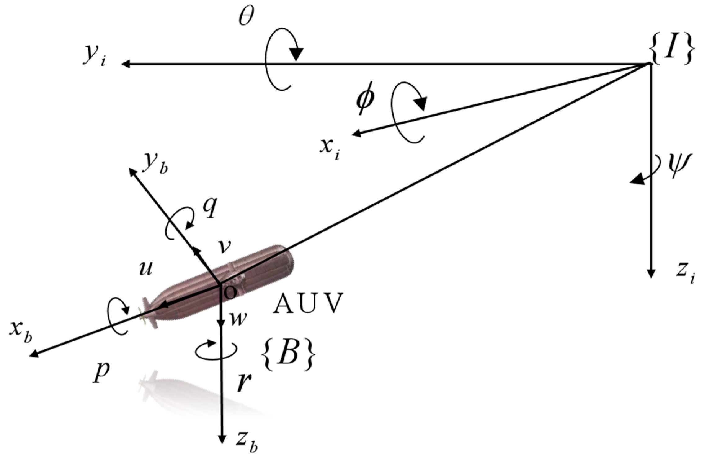
2.3. AUV Movement Model

According to Figure 1, the dynamics of AUVs are usually modeled by a six-degree-of-freedom (DOF) model. However, AUVs do not have actuators for rolling control, so rolling motion is usually not considered. In the inertial coordinate system and its own fixed coordinate system, according to (Fossen, 2011) [23], the kinematic and dynamical model of the AUV can be represented by five degrees of freedom as follows [23]:

$$\left\{\begin{array}{l}\dot{\mathit{\eta }}=\mathit{R}(\psi ,\theta )v\\ \mathit{M}\dot{\mathit{v}}+\mathit{C}(\mathit{v})\mathit{v}+\mathit{D}(\mathit{v})\mathit{v}+\mathit{g}(\mathit{\eta })=\mathit{T}\end{array}\right.$$

(8)

where $\mathit{\eta }={\left[x,y,z,\theta ,\psi \right]}^T$, and $\mathit{v}={\left[u,v,w,q,r\right]}^T$. $\mathit{R}(\psi ,\theta )$ is the Jacobian coefficient from the body-fixed frame to the earth-fixed frame. $\mathit{M}$ is the inertia matrix, $\mathit{C}(\mathit{v})$ is the hydrodynamic Coriolis and centripetal force matrix, $\mathit{D}(\mathit{v})$ is the nonlinear fluid hydrodynamic damping matrix, $\mathit{g}(\mathit{\eta })$ is the restoring force (moment) vector, and $\mathit{T}$ is the external force and external moment vector applied to the vehicle.

The navigator system itself is strongly coupled and vulnerable to the influence of external waves and currents. The nonlinear characteristics of the navigator cause some difficulties in engineering processing, so this paper linearizes the model of the navigator with feedback.

First, the AUV dynamics can be expressed as a general nonlinear system [22].

$$\begin{array}{l}\dot{\mathit{x}}(t)=\mathit{f}\left(\mathit{x}(t)\right)+\mathit{g}\left(\mathit{x}(t)\right)\mathit{u}(t)\\ \mathit{y}(t)=\mathit{h}\left(\mathit{x}(t)\right)\end{array}$$

(9)

where $\mathit{x}\in {\mathbb{R}}^{\mathrm{m}}$ is the system state vector, $\mathit{u}\in {\mathbb{R}}^{\mathrm{p}}$ is the system control input vector, and $\mathit{y}\in {\mathbb{R}}^{\mathrm{q}}$ is the system output vector. $\mathit{f}(\mathit{x})$, $\mathit{g}(\mathit{x})$ and $\mathit{h}(\mathit{x})$ are the corresponding system vector coefficients.

Non-singular damping matrix ${\mathit{M}}_x$ can be defined as

$${\mathit{M}}_x=\left[\begin{array}{cc}\mathit{I}& 0\\ 0& {\mathit{M}}_c\end{array}\right]$$

(10)

where ${\mathit{M}}_c\in {\mathbb{R}}^{5\times 5}$ stands for the hydrodynamic added mass of the related AUV model [22].

The system function $\mathit{f}(\mathit{x})$ and $\mathit{g}(\mathit{x})$ can be expressed as

$$\left\{\begin{array}{l}\mathit{f}\left(\mathit{x}\right)={\mathit{M}}_x^{-1}{\mathit{f}}^{\prime }\left(\mathit{x}\right)\\ \mathit{g}\left(\mathit{x}\right)={\mathit{M}}_x^{-1}{\mathit{g}}^{\prime }\left(\mathit{x}\right)\end{array}\right.$$

(11)

The output equation of the system can be defined as

$$\mathit{h}(\mathit{x})={\left[\begin{array}{lllll}x\hfill & y\hfill & z\hfill & \theta \hfill & \psi \hfill \end{array}\right]}^{\mathrm{T}}$$

(12)

Based on the nonlinear model of an AUV and the principle of feedback linearization, the feedback control rate and the set of coordinate transformations are found to obtain the feedback linearization model of the unmanned aerial vehicle.

The system function vector $\mathit{f}(\mathit{x})$, $\mathit{h}(\mathit{x})$, $\mathit{g}(\mathit{x})$ can be obtained from the previous presentation.

$$\mathit{f}(\mathit{x})={\mathit{M}}_x^{-1}{\mathit{f}}^{\prime }(x)=\left[\begin{array}{cc}\mathit{I}& 0\\ 0& {\mathit{M}}_c^{-1}\end{array}\right]\left[\begin{array}{c}\mathit{R}(\mathit{\eta })\mathit{v}\\ \mathit{N}(\mathit{\eta },\mathit{v})\end{array}\right]$$

(13)

$$\mathit{h}(\mathit{x})={\left[h_1(x),h_2(x),h_3(x),h_4(x),h_5(x)\right]}^{\mathrm{T}}={\left[x,y,z,\theta ,\psi \right]}^{\mathrm{T}}$$

(14)

$$\mathit{g}(\mathit{x})=\left[{\mathit{g}}_1(\mathit{x}),{\mathit{g}}_2(\mathit{x}),\cdots ,{\mathit{g}}_5(\mathit{x})\right]=\left[\begin{array}{c}\mathit{0}\\ {\mathit{M}}^{-1}{\mathit{g}}^{\prime }(\mathit{x})\end{array}\right]$$

(15)

where, $\mathit{0}$ is a $5\times 5$ zero matrix.

Based on the Lee derivative [24] and the definition of $\mathit{g}(\mathit{x})$, for any $1\le i\le 10$, $1\le j\le 10$, it follows that

$$L_{g_i}{h}_j(x)=0$$

(16)

By calculating the above equation, we can obtain the matrix $\mathsf{\Gamma }(\mathit{x})=[{\mathsf{\Gamma }}_{ij}(\mathit{x})]$, ${\mathsf{\Gamma }}_{ij}(\mathit{x})=L_{g_j}{L}_f{h}_i(x)$ and $1\le i\le p,1\le j\le p$ where matrix $\mathsf{\Gamma }(\mathit{x})$ is a non-singular matrix, and ${\rho }_1+{\rho }_2+{\rho }_3+{\rho }_4+{\rho }_5=10$. The relative order is the same as the system order, i.e., the nonlinear model of the navigator can be linearized by feedback. By transforming $z=\phi (x)$ by coordinates, it follows that

$$\begin{array}{l}{\mathit{x}}_i={\left[\begin{array}{lllll}{h}_1(x)\hfill & h_2(x)\hfill & h_3(x)\hfill & h_4(x)\hfill & h_5(x)\hfill \end{array}\right]}^{\mathrm{T}}\\ {\mathit{v}}_i={\left[\begin{array}{lllll}{L}_f{h}_1(x)\hfill & L_f{h}_2(x)\hfill & L_f{h}_3(x)\hfill & L_f{h}_4(x)\hfill & L_f{h}_5(x)\hfill \end{array}\right]}^{\mathrm{T}}\end{array}$$

(17)

Based on the definition of the Lee derivative,

$$\begin{array}{l}{\dot{\mathit{x}}}_i={\mathit{v}}_i\\ {\dot{\mathit{v}}}_i=L_f^2\mathit{h}(\mathit{x})+L_g{L}_f\mathit{h}(\mathit{x})\mathit{u}\end{array}$$

(18)

Control inputs in the new coordinate system:

$$\mathit{u}=\mathit{B}(x)+\mathsf{\Gamma }(x)\mathit{u}=L_f^2\mathit{h}(x)+L_g{L}_f\mathit{h}(x)\mathit{u}$$

(19)

In the presence of a transformed coordinate system and feedback control inputs:

$$\tilde{\mathit{u}}={\mathsf{\Gamma }}^{-1}(x)(\mathit{u}-\mathit{B}(x))$$

(20)

To sum up, the standard feedback linearization dynamic second-order integral model of an AUV could be reorganized as follows:

$$\begin{array}{l}{\dot{\mathit{x}}}_i(t)={\mathit{v}}_i(t)\\ {\dot{\mathit{v}}}_i(t)={\tilde{\mathit{u}}}_i(t)\end{array}$$

(21)

where ${\mathit{x}}_i\in {\mathbb{R}}^5$, ${\mathit{v}}_i\in {\mathbb{R}}^5$, and ${\mathit{u}}_i\in {\mathbb{R}}^5$.

2.4. Formation Communication Topology

In the consistency control of the AUV formation, there are $n$ AUVs among the formation members, and the communication relationship between the formations is represented as $G(U,\epsilon ,\mathit{A})$. $U$ indicates a single member of the formation. $\mathit{\epsilon }$ denotes all communication chains. $\mathit{A}$ denotes the adjacency matrix of the formation communication relationship. The Laplace matrix is defined as $\mathit{L}=\mathit{D}(G)-\mathit{A}(G)$ where $\mathit{D}(G)=diag(d(i))$ denotes its entry-degree matrix. $d(i)$ is the number of AUVs that can transmit information to any single $U$ in the formation AUV. If the AUV formation members can communicate in both directions, based on the principle of the graph theory, it is indicated that graph A is an undirected graph, as shown in Figure 2 [24].

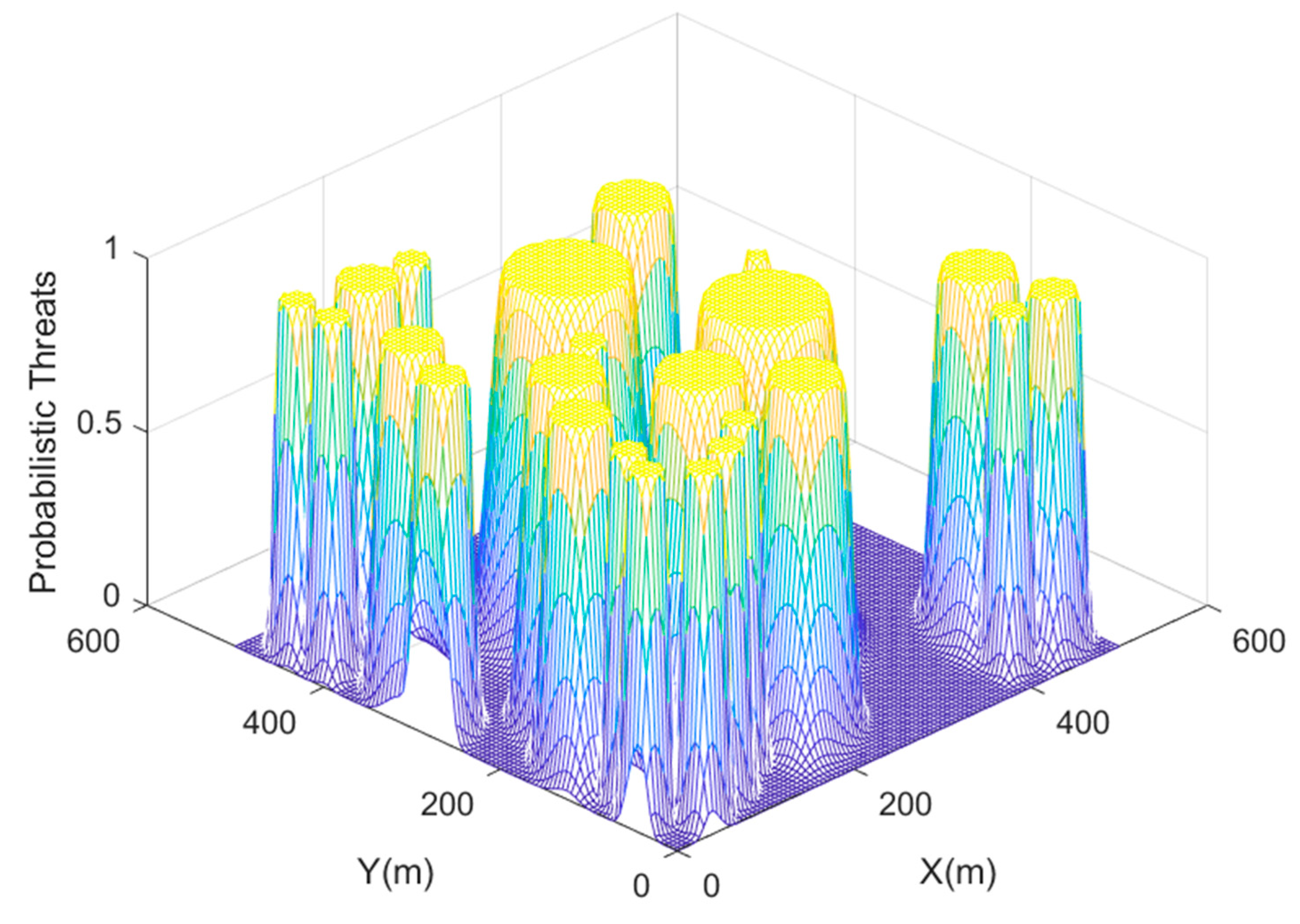
2.5. Probabilistic Threat Environment

To represent the threats to AUVs in complex subsea environments, probabilistic threat environment maps are defined in this paper to model them. The probabilistic threat map is a function of location and describes the threat probability of the threat sources at different locations to which the AUV is exposed [25]. It is an environment that shows the distribution of threats in the environment in a probabilistic form. Each location coordinate corresponds to a probability density value as an indication of the risk of AUV exposure to a threat source at that coordinate point. The following is a description of the probabilistic threat environment function model encountered by AUVs in this paper.

In the course of AUV formation navigation, underwater terrain and obstacle threats are threats that need to be completely avoided in the path-planning process. In this case, such threats are equated into a circular domain, and the probability threat value at each point decreases as it increases with the center of the circle. Therefore, a two-dimensional Gaussian distribution function model can be used to model the threat. For a threat source modeled by a Gaussian distribution, two characteristic parameters are needed to represent the threat source [26]: one that indicates the mean parameter of the centroid of the modeled threat source as $\mathit{\mu }$ and one that indicates the variance value of the modeled threat area of action ${\mathit{K}}_i$. The threat source modeled by a Gaussian distribution can be expressed as

$$f(r)=\frac{1}{2\pi \sqrt{\det ({\mathit{K}}_i)}}\exp \left[-\frac{1}{2}{(\mathit{r}-\mathit{\mu })}^{\mathrm{T}}{\mathit{K}}_i(\mathit{r}-\mathit{\mu })\right]$$

(22)

where $\mathit{\mu }=\left[\begin{array}{c}{\mu }_x\\ {\mu }_y\end{array}\right],{\mathit{K}}_i=\left[\begin{array}{cc}{\sigma }_x^2& 0\\ 0& {\sigma }_y^2\end{array}\right]$.

Suppose there are m suspicious locations in the region, the threat probability for any location $\mathit{r}$ in the region can be expressed as a multidimensional Gaussian probability function:

$$threat(\mathit{r})={\displaystyle \sum _{i=1}^m\frac{1}{2\pi \sqrt{\det ({\mathit{K}}_i)}}}\exp [-\frac{1}{2}{(\mathit{r}-{\mathit{r}}_i)}^{\mathrm{T}}{\mathit{K}}_i(\mathit{r}-{\mathit{r}}_i)]$$

(23)

The probabilistic threat environment represented by a multidimensional Gaussian probability function can be shown in Figure 3.

3. Improvement of Artificial Potential Field Method

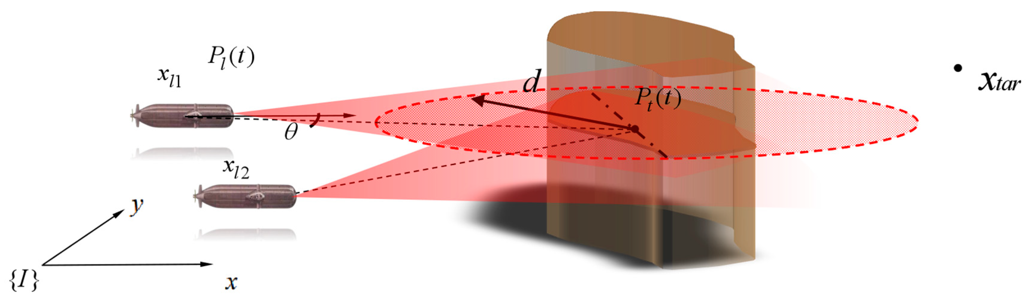
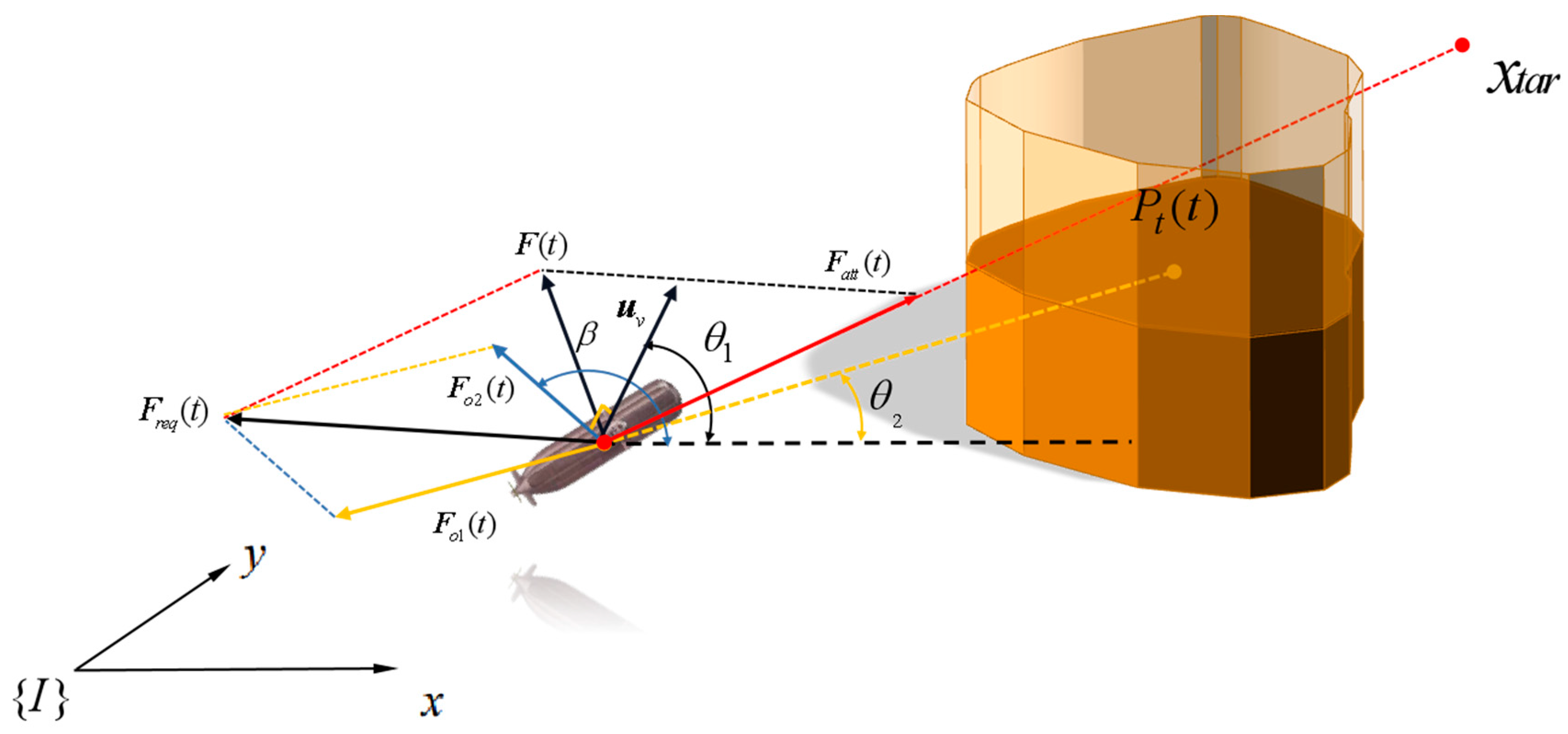
3.1. Auxiliary Potential Field Repulsion Field Design for Obstacles

The artificial potential field method is widely used in the scenario of local obstacle avoidance, which has the advantages of good real time and does not rely on global information [27]. However, it has disadvantages such as the overlapping potential fields of adjacent obstacles and the fact that it can easily fall into local minima. This will prevent the AUV from obtaining the optimal path. During the control of the AUV, the time for the AUV obstacle avoidance operation command is insufficient due to the missing longitudinal control of the AUV. Based on the shortcomings of the traditional artificial potential field method, we designed an obstacle-assisted potential field on the traditional artificial potential field method to avoid falling into local minima due to zero combined forces.

According to Figure 4, the obstacle reference point in the same plane as the AUV is defined as $p_t(t)=(x(t),y(t),z(t))$. The coordinate of the target point is defined as $x_{tar}(x_{tar},y_{tar},z_{tar})$. The current position of the AUV is denoted as ${\mathit{p}}_l(t)=[x_l(t),y_l(t),z_l(t)]$.

The repulsive force generated by the obstacle point on the AUV is ${\mathit{F}}_{o1}(t)$. The repulsive force generated by the auxiliary potential field on the AUV is ${\mathit{F}}_{o2}(t)$. The attraction of the target point to the AUV is ${\mathit{F}}_{att}(t)$. The coordination control within the AUV is ${\mathit{F}}_{in}(t)$.

In a probabilistic threat environment, the probabilistic threat value of the obstacle also affects the potential energy function of the AUV. The potential energy function varies with the transformation of the probabilistic threat value at the current location. With a time-varying distance vector, the potential energy function at the current position of the AUV at the current time can be expressed as

$$\mathit{U}=threat(\mathit{r})={\displaystyle \sum _{i=1}^m\frac{1}{2\pi }}\exp [-\frac{1}{2}{({\mathit{r}}_i)}^{\mathrm{T}}{\mathit{K}}_i({\mathit{r}}_i)]$$

(24)

The potential energy function with reference to the barrier point:

$${\mathit{U}}_{req}{}_1({\mathit{p}}_t(t))=\left\{\begin{array}{l}{\gamma }^2\exp \left\{-\frac{1}{2}{({\mathit{p}}_l(t)-{\mathit{p}}_t(t))}^{\mathrm{T}}{\mathit{K}}_{\mathit{i}}({\mathit{p}}_l(t)-{\mathit{p}}_t{(t)}_{\mathit{i}})\right\} △l\le d\\ 0△l>d\end{array}\right.$$

(25)

where $\gamma$ denotes the potential energy function coefficient, ${\mathit{K}}_i$ is the diagonal matrix indicating the threat intensity at the obstacle reference point, $△l=\left|p_l(t)-p_t(t)\right|$ is expressed as the distance between the AUV and the obstacle reference point, and d is the radius of the potential field action.

The potential energy function based on the reference barrier point yields the following gradient function:

$${\mathit{F}}_{o1}(t)=-\nabla {\mathit{U}}_{req1}({\mathit{p}}_l(t))=-\left\{\begin{array}{l}\left[\begin{array}{cc}\frac{\partial U_{req}({\mathit{p}}_l(t))}{\partial △x}& \frac{\partial U_{req}(p_l(t))}{\partial △y}\end{array}\right] △l\le d\\ 0△l>d\end{array}\right.$$

(26)

In order to prevent the AUV from falling into a local optimal solution, the artificial potential field method is improved here by constructing an obstacle-assisted potential field [28]. As shown in Figure 5, the direction of the potential field force of the auxiliary obstacle is perpendicular to the direction of travel of the AUV. The angle formed with the AUV is ${\theta }_1$.

Obstacle-assisted potential energy function $U_{req2}(p_t(t))$ is designed as

$${\mathit{U}}_{req2}({\mathit{p}}_t(t))=\frac{1}{2}{g}_v{(1+v)}^2{\mathit{R}}_{req2}^v(\beta )$$

(27)

where $g_v=k_o^2(1+r_n)$ is the random adjustment gain of the auxiliary potential field function. $k_o^2$ is the gain adjustment factor. $0\le r_n\le 1$; $r_n$ indicates a random number between 0 and 1. ${\mathit{R}}_{req2}^v(\beta )={[\begin{array}{cc}{\mathit{R}}_1& {\mathit{R}}_2\end{array}]}^T$ is expressed as the potential field transformation angle matrix where ${\mathit{R}}_1={[\begin{array}{cc}\cos (\beta )& \sin (\beta )\end{array}]}^T$, and ${\mathit{R}}_2={[-\sin (\beta )\cos (\beta )]}^T$.

$\beta$ indicates the rotation angle, which is related to the speed of the AUV itself and the relative angle of the obstacle. As shown in Figure 3, at this point $0<{\theta }_1-{\theta }_2<\pi /2$. The direction of the potential field force is a $\pi /2$ clockwise rotation of the current bow of the AUV in the direction of velocity.

$$\beta =\left\{\begin{array}{c}{\theta }_1+\pi /2\hspace{1em}\hspace{1em}\hspace{1em}0<{\theta }_1-{\theta }_2\le \pi /2\hfill \\ {\theta }_1-\pi /2\hspace{1em}\hspace{1em}\hspace{1em}-\pi /2<{\theta }_1-{\theta }_2\le 0\hfill \\ \hspace{1em}0\hspace{1em}\hspace{1em}\hspace{1em}\hspace{1em}\hspace{1em}\hspace{1em}\hspace{1em}else\hfill \end{array}\right.$$

(28)

The potential energy function based on the auxiliary potential field yields the following gradient function:

$${\mathit{F}}_{o2}(t)=-\nabla U_{req2}({\mathit{p}}_t(t))=g_v{(1+v)}^2{\mathit{R}}_{req2}^v(\beta ){\overrightarrow{\mathit{n}}}_v$$

(29)

where the unit vector of the current velocity direction of the navigator is denoted as ${\overrightarrow{\mathit{n}}}_v$.

The repulsion control input ${\mathit{F}}_{req}(t)$ is denoted as

$${\mathit{F}}_{req}(t)={\mathit{F}}_{o1}(t)+{\mathit{F}}_{o2}(t)$$

(30)

3.2. Gravitational Field Design for Target Points

Based on the artificial potential field method, it is known that the target point will exert a gravitational effect on the AUV formation, and the potential energy function of the target point on the current AUV is denoted as

$${\mathit{U}}_{att}(p_l(t))=\frac{\kappa }{{\lambda }^2}\rho ({\mathit{p}}_l(t),{\mathit{x}}_{tar})+\frac{\kappa }{\rho ({\mathit{p}}_l(t),{\mathit{x}}_{tar})+\lambda }$$

(31)

where $\lambda ,\kappa$ denotes the positive coefficient of the potential energy function.

The gradient of the potential energy function based on the target point is

$$\nabla {\mathit{U}}_{att}({\mathit{p}}_l(t))=\frac{\partial U_{att}({\mathit{p}}_l(t))}{\partial \rho }{\overrightarrow{\mathit{n}}}_{att}$$

(32)

where ${\overrightarrow{\mathit{n}}}_{att}$ is the unit vector from the navigator to the target point:

$$\frac{\partial U_{att}({\mathit{p}}_l(t))}{\partial \rho }=\frac{\kappa }{{\lambda }^2}-\frac{\kappa }{{(\rho ({\mathit{p}}_l(t),{\mathit{x}}_{tar})+\lambda )}^2}$$

(33)

$${\overrightarrow{\mathit{n}}}_{att}=\frac{{\mathit{p}}_l(t)-{\mathit{x}}_{tar}}{‖{\mathit{p}}_l(t)-{\mathit{x}}_{tar}‖}$$

(34)

Gravity control input ${\mathit{F}}_{att}(t)$ is denoted as

$${\mathit{F}}_{att}(t)=-\nabla {\mathit{U}}_{att}({\mathit{p}}_l(t))$$

(35)

The potential energy gradient function of the target point can be regarded as a constant value because the target point is at a location far from the AUV, and the potential energy gradient function of the target point remains essentially constant.

3.3. Coordination and Control within the Formation

In order to ensure the overall robustness of the formation, it should be less likely to have obvious formation changes due to the disturbance of the external environment and obstacle avoidance behavior, the risk of AUVs colliding with each other within the formation should be reduced, it should be ensured that the AUVs can converge stably, based on the communication structure in the formation AUVs, and the coordination control force within the formation should be based on the position and velocity state information of each AUV [29].

$${\mathit{F}}_{in}(t)=-\omega {\mathit{x}}_i(t)+{\mathit{K}}_{in}\left[{\mathit{K}}_p{\displaystyle \sum _{j\in N_i^x}{a}_{ij}(t)({\mathit{x}}_j-{\mathit{x}}_i)}+{\mathit{K}}_v{\displaystyle \sum _{j\in N_i^v}{b}_{ij}(t)}({\mathit{v}}_j-{\mathit{v}}_i)\right]$$

(36)

where ${\mathit{K}}_{in}$ and $\omega$ denote the control gain of the formation coordination control input. $a_{ij}(t)$ and $b_{ij}(t)$ are the communication weights within the system. ${\mathit{K}}_p$ and ${\mathit{K}}_v$ denote the control gains in the position and velocity communication topologies, respectively.

Based on the forces on the AUV in the potential field, the control input $\mathit{F}(t)$ to the AUV can be expressed as

$$\mathit{F}(t)={\mathit{F}}_{att}(t)+{\mathit{F}}_{req}(t)+{\mathit{F}}_{in}(t)$$

(37)

3.4. Algorithm Flow of Cooperative Obstacle Avoidance

The AUV formation is controlled by the formation clustering algorithm to complete the overall movement of the formation before the threat is perceived [30]. When a threatening obstacle is encountered, the above-mentioned obstacle avoidance algorithm is used to successfully avoid the high-threat obstacle by multi-beam sonar sensing, and the improved artificial potential field algorithm is used to return to the cluster formation control after removing the obstacle.

Based on (21), the second-order integral model of an AUV is denoted as

$$\begin{array}{l}{\dot{\mathit{x}}}_i(t)={\mathit{v}}_i(t)\\ {\dot{\mathit{v}}}_i(t)={\tilde{\mathit{u}}}_i(t)\end{array}$$

(38)

The actual position and velocity state information during the AUV voyage can be expressed as ${\mathit{D}}_i(\mathit{x})={[x_i(t),{\mathit{v}}_i(t)]}^T$. The desired time-varying formation state is expressed as ${\overline{\mathit{D}}}_i(x)={[{\overline{\mathit{x}}}_i(t),{\overline{\mathit{v}}}_i(t)]}^T$. The pre-command generates the initial desired formation, and the desired formation is modified by the modified artificial potential field method above when the AUV cluster system senses an obstacle. The corrected desired formation is denoted as $\overline{\mathit{H}}(x)=\overline{\mathit{D}}(x)+\mathit{F}(x)$, where $\mathit{F}(x)=-\nabla {\mathit{U}}_{req}({\mathit{x}}_i(t))-\nabla {\mathit{U}}_{att}({\mathit{x}}_i(t))$.

The consistency protocol at this point is denoted as

$${\tilde{\mathit{u}}}_i(t)=\mathit{F}(\mathit{x})+{\mathit{K}}_1({\mathit{D}}_i(x)-{\overline{\mathit{H}}}_i(t))+{\mathit{K}}_2{\displaystyle \sum _{j\in N_i}{w}_{ij}(({\mathit{D}}_j(x)-{\overline{\mathit{H}}}_j(t))-({\mathit{D}}_i(x)-{\overline{\mathit{H}}}_i(t))}$$

(39)

where ${\mathit{K}}_1={\mathit{K}}_{in}{\mathit{K}}_p$, ${\mathit{K}}_2={\mathit{K}}_{in}{\mathit{K}}_v$, and $w_{ij}$ indicates the coefficient of the effect of the current position on its motion state.

The AUV formation cooperative obstacle avoidance algorithm flow is shown in Figure 6. The obstacle avoidance algorithm in this paper adopts the strategy of disbanding the formation and reconfiguring the formation to solve the control problem of the cluster before and after obstacle avoidance; that is, the AUV formation is controlled by the cluster formation algorithm to complete the control of the whole formation movement behavior when it does not encounter an obstacle; the AUV switches to the obstacle avoidance algorithm when it encounters an obstacle, and the AUV relies on its own sensor data and the artificial potential field algorithm to complete obstacle avoidance. After the AUV formation leaves the obstacle terrain, it returns to the cluster formation control and continues to perform operational tasks.

4. Stability Analysis

The different potential field effects due to the obstacle space produce different directional forces in the formation system. It causes the AUV to produce obstacle avoidance routes in different directions [31]. In this paper, the AUV formation system will form two small subsystems. The total number of AUVs in the two subsystems is m. The number of AUVs in the two subsystems is $m_1$ and $m_2$, respectively, and $m_1+m_2=m$.

The stability of the system can be proven by constructing an energy function. The energy functions of the two systems are defined as $W_1(V(t),X(t))$ and $W_2(V(t),X(t))$, respectively. $V(t)$ is denoted as the velocity energy function, $X(t)$ is denoted as the position energy primary function, and $\eta (V(t))$ is denoted as the sum of the energies of the subsystem potential fields.

$$W_1(V_i(t),X_i(t))=V_i(t)+X_i(t)+2{\eta }_1(V_i(t))$$

(40)

$$W_2(V_j(t),X_j(t))=V_j(t)+X_j(t)+2{\eta }_2(V_j(t))$$

(41)

where $V_i(t)={\displaystyle \sum _{i=1}^{m_1}{\mathit{v}}_i^{\mathrm{T}}}{\mathit{v}}_i(t)$, $X_i(t)=\omega {\displaystyle \sum _{i=1}^{m_1}{\mathit{x}}_i^{\mathrm{T}}}{\mathit{x}}_i(t)$, ${\eta }_1(V_i(t))={\displaystyle \sum _{i=1}^{m_1}(U_{req}^i(\mathit{x}(t))+U_{att}^i(x(t)))}$, $V_j(t)={\displaystyle \sum _{j=1}^{m_2}{\mathit{v}}_j^{\mathrm{T}}}{\mathit{v}}_j(t)$, $X_j(t)=\omega {\displaystyle \sum _{j=1}^{m_2}{\mathit{x}}_i^{\mathrm{T}}}{\mathit{x}}_i(t)$, and ${\eta }_2(V_j(t))={\displaystyle \sum _{j=1}^{m_2}(U_{req}^j(\mathit{x}(t))+U_{att}^j(x(t)))}$.

The two subsystems are similar in the formation process and the stability proof process. In this section, only one subsystem stability proof is carried out, and the conclusion is given.

Theorem 1.

The initial energy function of the system includes the velocity energy function, the position energy function and the sum of the energy of the potential field. Then, the initial energy function A of the system is bounded, and then the formation can be transformed by autonomous formation, and the following conclusion holds: in the process of formation avoidance, the splitting transformation of the formation is generated, and the subsystem always keeps converging.

$${\dot{W}}_1(V(t),X(t))<0,{\dot{W}}_2(V(t),X(t))<0$$

(42)

Proof. 

The subsystem energy function is derived as follows:

$${\dot{W}}_1(V(t),X(t))=2{\displaystyle \sum _{i=1}^{m_1}{\mathit{v}}_i^T(t){\dot{\mathit{v}}}_i(t)}+2\omega {\displaystyle \sum _{i=1}^{m_1}{\mathit{x}}_i^T(t){\dot{\mathit{x}}}_i(t)}+2{\dot{\eta }}_1(\zeta (t))$$

(43)

Equation (39) is substituted into (43):

$$\begin{array}{ll}{\dot{W}}_1(V(t),X(t))=& 2{\displaystyle \sum _{i=1}^{m_1}{\mathit{v}}_i^T(t)(-{\nabla }_l{\psi }_t-{\nabla }_l{\psi }_o-\omega {\mathit{x}}_i(t))}\\ & +2{\displaystyle \sum _{i=1}^{m_1}{\mathit{v}}_i^T(t)\left({\mathit{K}}_{in}^p{\displaystyle \sum _{j\in N_i^x}{a}_{ij}}(t)({\mathit{x}}_j-{\mathit{x}}_i)+{\mathit{K}}_{in}^v{\displaystyle \sum _{j\in N_i^x}{b}_{ij}}(t)({\mathit{v}}_j-{\mathit{v}}_i)\right)}\\ & +2{\dot{\eta }}_1(V(t))+2\omega {\displaystyle \sum _{i=1}^{m_1}{\mathit{x}}_i^T(t){\mathit{v}}_i(t)}\end{array}$$

(44)

Since ${\mathit{v}}_i(t)$ and ${\mathit{x}}_i(t)$ are column vectors of the same dimension, there exists ${\mathit{x}}_i^{\mathrm{T}}(t){\mathit{v}}_i(t)={\mathit{v}}_i^{\mathrm{T}}(t){\mathit{x}}_i(t)$. □

$$\begin{array}{ll}{\dot{W}}_1(V(t),X(t))=& -2{\displaystyle \sum _{i=1}^{m_1}{\mathit{v}}_i^{\mathrm{T}}(t)({\nabla }_l{\psi }_t+{\nabla }_l{\psi }_o)}\\ & +2{\displaystyle \sum _{i=1}^{m_1}{\mathit{v}}_i^{\mathrm{T}}(t){\mathit{K}}_{in}^p{\displaystyle \sum _{j\in N_i^x}{a}_{ij}}(t)({\mathit{x}}_j-{\mathit{x}}_i)}\\ & +2{\displaystyle \sum _{i=1}^{m_1}{\mathit{K}}_{in}^v{\displaystyle \sum _{j\in N_i^x}{b}_{ij}}(t)({\mathit{v}}_j-{\mathit{v}}_i)+2{\dot{\eta }}_1(\mathit{x}(t))}\end{array}$$

(45)

The derivative of the total potential energy function of the subsystem can be obtained from its definition.

$${\dot{\eta }}_1(V(t))={\left({\displaystyle \sum _{i=1}^{m_1}({\psi }_o^i(△l)+{\psi }_t^i}(△l))\right)}^{\prime }=X(t){\displaystyle \sum _{i=1}^{m_1}({\nabla }_l{\psi }_o^i)}+X(t){\displaystyle \sum _{i=1}^{m_1}({\nabla }_l{\psi }_t^i(△l))}$$

(46)

Equation (46) is substituted into (43):

$${\dot{W}}_1(V(t),X(t))=-2X^{\mathrm{T}}(t)\left({\mathit{L}}_p\otimes {\mathit{K}}_{in}^p\right)V(t)-2X^{\mathrm{T}}(t)\left({\mathit{L}}_p\otimes {\mathit{K}}_{in}^v\right)X(t)$$

(47)

Lemma 1.

When$x\in {\mathbb{R}}^n$,$y\in {\mathbb{R}}^n$, and$\beta >0$, there exists the following inequality that holds:

$${\mathit{x}}^{\mathrm{T}}\mathit{y}+{\mathit{y}}^{\mathrm{T}}\mathit{x}\le \beta {\mathit{x}}^{\mathrm{T}}\mathit{x}+{\beta }^{-1}{\mathit{y}}^{\mathrm{T}}\mathit{y}$$

(48)

Based on the above lemma, the following inequalities exist:

$$-2X^{\mathrm{T}}(t)\left({\mathit{L}}_p\otimes {\mathit{K}}_{in}^p\right)V(t)\le -\delta X^{\mathrm{T}}(t)-V^{\mathrm{T}}(t){\left({\mathit{L}}_p\otimes {\mathit{K}}_{in}^p\right)}^{\mathrm{T}}\left({\mathit{L}}_p\otimes {\mathit{K}}_{in}^p\right)V(t)$$

(49)

Equation (47) is substituted into (49):

$${\dot{W}}_1(V(t),V(t))\le -\delta {\mathrm{ X}}^{\mathrm{T}}(t)X(t)-{\mathrm{ V}}^{\mathrm{T}}(t)\mathsf{\Theta }V(t)$$

(50)

where $\mathsf{\Theta }={\left({\mathit{L}}_p\otimes {\mathit{K}}_{in}^p\right)}^{\mathrm{T}}\left({\mathit{L}}_p\otimes {\mathit{K}}_{in}^p\right)+2\left({\mathit{L}}_p\otimes {\mathit{K}}_{in}^v\right)$.

According to the properties of the Laplacian matrix, it must be a vivacious semi-definite matrix. From this, it can be deduced that the formation must be able to converge stably.

5. Simulation Verification and Analysis

The following simulation example verifies the effectiveness of the research on the multi-AUV coordinated obstacle avoidance method based on the improved artificial potential field method and the consistency protocol algorithm. Since this paper conducts the study of the local obstacle avoidance problem of AUV formation, only local threat environment modeling is performed when designing the environment.

The simulation considers four AUV formation systems that can communicate with each other, and its communication topology is shown in Figure 2. Then, its Laplace matrix is

$${\mathit{ L}}_p=\left[\begin{array}{cccc}2& -1& -1& 0\\ -1& 2& 0& -1\\ -1& 0& 2& -1\\ 0& -1& -1& 2\end{array}\right]$$

(51)

The initial position status information of each AUV is $x_i\in [0,50]$, $y_i\in [0,140]$, and $i\in \left\{1,2,3,4\right\}$. The initial velocity of the AUV is 0. Probabilistic threat intensity diagonal matrix ${\mathit{K}}_i$ is $0.002I_{3\times 3}$. Potential field coefficient $\gamma =1,\kappa =0.1,\lambda =1$. Obstacles are randomly distributed in the map. The target points for the cooperative operation of the AUV formation are $[300,y_i,-5]$. After reaching consistency, the distance between the formation AUVs is maintained at 10 m.

Figure 7 gives the paths of the formation AUVs in the process of coordinated obstacle avoidance. The formation AUVs feel different threat levels and decelerate differently after entering the potential field area, but each keeps a relative distance between the formations, and no collision behavior occurs, and finally, the formation achieves consistency according to the consistency protocol.

Figure 8, Figure 9 and Figure 10 show the changes in position attitude and each velocity state during the formation dissolution, formation coordinated obstacle avoidance process and formation reconfiguration process of multi-AUVs in the face of obstacles, respectively. From Figure 8, it can be seen that the spatial position relationship of the AUV formation in the formation system can still converge after passing through the potential field region and generating the separation of obstacle avoidance actions. In Figure 9 and Figure 10, the motion states of each AUV show a similar converge–separate–converge pattern as the potential field appears.

Based on the comprehensive simulation results above, it can be judged that the algorithm based on the improved artificial potential field method and consistency protocol proposed in this chapter can effectively solve the problem of multi-AUV coordinated obstacle avoidance and ensure the convergence and stability of the formation while ensuring the formation avoidance of obstacles and formation change.

6. Discussion

The improved artificial potential field method presented in this paper is partially applicable to the obstacle avoidance control of a single AUV when the virtual gravitational force F_in(t) among the formation members is neglected. When the AUV formation faces multiple obstacles, different coverage circle domains can be constructed separately for the obstacles, and there may be an overlap of exclusion regions between the obstacles. In this way, the path of the formation is not optimal because the submersible cannot enter the region. Therefore, for the AUV formation path optimization problem in a complex obstacle environment, relevant algorithms for the real-time dynamic obstacle avoidance and path optimization of the submersible formation can be constructed in the future by combining the construction of a local path optimization algorithm with the improved artificial potential field method introduced above.

7. Conclusions

For the local obstacle avoidance problem of AUV formations, we proposed a cooperative obstacle avoidance algorithm based on an improved artificial potential field method and a consistency protocol. Firstly, for the disadvantage that the traditional artificial potential field method can easily fall into local minima, an auxiliary potential field perpendicular to the AUV moving direction was designed to solve the problem that AUVs can easily have zero combined force in the potential field and local minima. Secondly, for the problem that the formation will change during local obstacle avoidance, an AUV formation control method that keeps the speed and position consistent was designed. The control conflict problem of the combined algorithm of the artificial potential field law and the consistency protocol was solved by adjusting the desired formation of the consistency protocol through the potential field force. Finally, the stability of system convergence was demonstrated by a bounded energy function. We verified by simulation that the AUV formation can achieve convergence of the formation state in the case of the local obstacle avoidance method proposed in the paper. The effectiveness of the proposed algorithm is confirmed.

References

1. Antonelli, G. Underwater Robots; Springer: Berlin/Heidelberg, Germany, 2014; pp. 20–23. [Google Scholar]
2. Sahu, B.K.; Subudhi, B. Flocking control of multiple AUVs based on fuzzy potential functions. IEEE Trans. Fuzzy Syst. 2018, 26, 2539–2551. [Google Scholar] [CrossRef]
3. Xin, L.; Zhu, D. An adaptive SOM neural network method to distributed formation control of a group of AUVs. IEEE Trans. Ind. Electron. 2018, 65, 8260–8270. [Google Scholar]
4. Fu, J.; Sun, G. Trajectory Homotopy to Explore and Penetrate Dynamically of Multi-UAV. IEEE Trans. Intell. Transp. Syst. 2022, 23, 24008–24019. [Google Scholar] [CrossRef]
5. Dechter, R.; Pearl, J. Generalized best-first search strategies and the optimalityof A*. Assoc. Comput. Mach. 1985, 32, 505–536. [Google Scholar] [CrossRef]
6. Cobb, H.G.; Grefenstette, J. Genetic algorithms for tracking changing environments. In Proceedings of the International Genetic Algorithms Conference, San Francisco, CA, USA, 1 June 1993; Naval Research Lab: Washington, DC, USA, 1993; pp. 1–8. [Google Scholar]
7. Cui, R.X.; Li, Y.; Yan, W.S. Mutual information-based multi-AUV path planning for scalar field sampling using multidimensional RRT*. IEEE Trans. Syst. Man Cybern. Syst. 2016, 46, 993–1004. [Google Scholar] [CrossRef]
8. Eberhart, R.; Kennedy, J. A new optimizer using particle Swarm Theory. In Proceedings of the Sixth International Symposium on Micro Machine and Human Science, Nagoya, Japan, 4–6 October 1995; IEEE: Piscataway, NJ, USA, 1995; pp. 39–43. [Google Scholar]
9. Ma, Y.N.; Gong, Y.J.; Xiao, C.F.; Gao, Y.; Zhang, J. Path planning for autonomous underwater vehicles: An ant colony algorithm incorporating alarm pheromone. IEEE Trans. Veh. Technol. 2018, 68, 141–154. [Google Scholar] [CrossRef]
10. Noguchi, Y.; Maki, T. Path planning method based on artificial potential field and reinforcement learning for intervention AUVs. In 2019 IEEE Underwater Technology (UT); IEEE: Piscataway, NJ, USA, 2019; pp. 1–6. [Google Scholar]
11. Smith, S.M.; Ganesan, K.; An, P.E.; Dunn, S.E. Strategies for simultaneous multiple autonomous underwater vehicle operation and control. Int. J. Syst. Sci. 1998, 29, 1045–1063. [Google Scholar] [CrossRef]
12. Sun, B.; Zhu, D.Q.; Tian, C.; Luo, C.M. Complete coverage autonomous underwater vehicles path planning based on glasius bio-inspired neural network algorithm for discrete and centralized programming. IEEE Trans. Cogn. Dev. Syst. 2018, 11, 73–84. [Google Scholar] [CrossRef]
13. Yan, C.; Xiang, X.J.; Wang, C. Towards real-time path planning through deep reinforcement learning for a UAV in dynamic environments. J. Intell. Robot. Syst. 2020, 98, 297–309. [Google Scholar] [CrossRef]
14. Cheng, C.L.; Zhu, D.Q.; Sun, B.; Chu, Z.Z.; Nie, J.D.; Zhang, S. Path planning for autonomous underwater vehicle based on artificial potential field and velocity synthesis. In Proceedings of the IEEE 28th Canadian Conference on Electrical and Computer Engineering, Halifax, NS, Canada, 3–6 May 2015; pp. 717–721. [Google Scholar]
15. Song, J.; Hao, C.; Su, J.C. Path planning for unmanned surface vehicle based on predictive artificial potential field. Int. J. Adv. Robot. Syst. 2020, 17, 1729881420918461. [Google Scholar] [CrossRef]
16. Zhao, Z.Y.; Hu, Q. A cooperative hunting method for multi-AUV swarm in un-dewater weak in formation environment with Obstacles. J. Mar. Sci. Eng. 2020, 10, 1266. [Google Scholar] [CrossRef]
17. Wang, S.M.; Fang, M.C.; Hwang, C.N. Vertical obstacle avoidance and navigation of autonomous underwater vehicles with H infinity controller and the artificial potential field method. J. Navig. 2019, 72, 207–228. [Google Scholar] [CrossRef]
18. Zhen, Q.Z.; Wan, L.; Li, Y.L.; Jiang, D.P. Formation control of a multi-AUVs system based on virtual structure and artificial potential field on SE(3). Ocean. Eng. 2022, 253, 111148. [Google Scholar] [CrossRef]
19. Orozco-Rosas, U.; Montiel, O.; Sepulveda, R. Mobile robot path planning using membrane evolutionary artificial potential field. Appl. Soft Comput. 2021, 77, 236–251. [Google Scholar] [CrossRef]
20. Li, J.; Zhang, J.X.; Zhang, H.H.; Yan, Z.P. A predictive guidance obstacle avoidance algorithm for AUV in unknown environments. Sensors 2019, 19, 2862. [Google Scholar] [CrossRef]
21. Lin, X.G.; Tian, W.D.; Zhang, W. The leaderless multi-AUV system fault-tolerant consensus strategy under heterogeneous communication topology. Ocean. Eng. 2021, 237, 109594. [Google Scholar] [CrossRef]
22. Yan, Z.P.; Liu, Y.B.; Zhou, J.J.; Zhang, W.; Wang, L. Consensus of multiple autonomous underwater vehicles with double independent Markovian switching topologies and timevarying delays. Chin. Phys. B 2017, 26, 040203. [Google Scholar] [CrossRef]
23. Fossen, T.I. Handbook of Marine Craft Hydrodynamics and Motion Control; John Wiley and Son: Chichester, UK, 2011. [Google Scholar]
24. Li, J.; Zhang, H.D.; Chen, T.; Wang, J.Q. AUV Formation Coordination Control Based on Transformed Topology under Time-Varying Delay and Communication Interruption. J. Mar. Sci. Eng. 2022, 10, 950. [Google Scholar] [CrossRef]
25. Zhang, B.T.; Liu, Y.; Liu, Y.; Wang, J. A path planning strategy for searching the most reliable path in uncertain environments. Int. J. Adv. Robot. Syst. 2017, 13, 23–32. [Google Scholar] [CrossRef]
26. Johnson, P.; Vernotte, A.; Ekstedt, M.; Lagerstrom, R. pwnPr3d: An Attack-Graph-Driven Probabilistic Threat-Modeling Approach. In Proceedings of the 2016 11th International Conference on Availability, Reliability and Security (ARES), ARES 2016, Salzburg, Austria, 31 August–2 September 2016; pp. 278–283. [Google Scholar]
27. Khatib, O. Real-time obstacle avoidance for manipulators and mobile robots. Int. J. Robot. Res. 1986, 5, 90–98. [Google Scholar] [CrossRef]
28. Zhang, W.; Wei, S.L.; Zeng, J.; Wang, N.X. Multi-UUV path planning based on improved artificial potential field method. Int. J. Robot. Autom. 2021, 36, 231–239. [Google Scholar]
29. Chen, Y.L.; Ma, X.W.; Bai, G.Q.; Sha, Y.B.; Liu, J. Multi-autonomous underwater vehicle formation control and cluster search using a fusion control strategy at complex underwater environment. Ocean. Eng. 2021, 216, 108048. [Google Scholar] [CrossRef]
30. Liang, D.; Liu, Z.Y.; Bhamra, R. Collaborative Multi-Robot Formation Control and Global Path Optimization. Appl. Sci. 2022, 12, 7046. [Google Scholar] [CrossRef]
31. Civelek, C. Stability analysis of engineering/physical dynamic systems using residual energy function. Arch. Control Sci. 2019, 28, 201–222. [Google Scholar]
Figure 1. AUV model in 6-DOF.
Jmse 11 01157 g001
Figure 2. AUV formation communication topology flow.
Jmse 11 01157 g002
Figure 3. Probabilistic Threat Environment Map.
Jmse 11 01157 g003
Figure 4. AUV formation obstacle recognition.
Jmse 11 01157 g004
Figure 5. Based on obstacle-assisted potential field artificial potential field method.
Jmse 11 01157 g005
Figure 6. Formation cooperative obstacle avoidance algorithm flow.
Jmse 11 01157 g006
Figure 7. Multi-AUV formation obstacle avoidance path.
Jmse 11 01157 g007
Figure 8. Position state curve of multi-AUV.
Jmse 11 01157 g008
Figure 9. Linear velocity profile of multi-AUV.
Jmse 11 01157 g009
Figure 10. Attitude and angular velocity profile of multi-AUV.
Jmse 11 01157 g010
Disclaimer/Publisher’s Note: The statements, opinions and data contained in all publications are solely those of the individual author(s) and contributor(s) and not of MDPI and/or the editor(s). MDPI and/or the editor(s) disclaim responsibility for any injury to people or property resulting from any ideas, methods, instructions or products referred to in the content.