A Methodology to Design a Wind Transfer Function: Application to the Valdevaqueros Dune (SW Spain)

Abstract

In general, weather forecasting has been significantly developed at a large scale and, joined with statistical techniques, is used to predict at a local scale. However, there is no way to propagate winds between two nearby locations; this is a spatial transference, for example, for the waves. After studying coastal dunar systems affected by winds, we have proposed a way for the spatial propagation of wind for scales under 10 km. The proposed transference is based on local data, and it is developed in an easy and accurate way by different regression methods and the wind profile theory. The aim of this article is to establish a methodology for achieving a wind transfer function for local applications. For this purpose, we analyzed and compared data from a field experiment and from a nearby weather station. A combination of the wind profile and statistical downscaling technique formed the basis of this research, which leads to transfer equations for wind speeds and directions. To clarify the procedure, the proposed methodology was applied to the Valdevaqueros Coastal Dune in order to develop a transfer function using time series data from a nearby meteorological station located in Tarifa.

1. Introduction

There are different techniques focused on weather prediction, but only a few of them apply to the aims of this study, spatial wind transference at a local scale. Statistical downscaling (SD) is the technique used for reduced areas (up to 10 km) at different time scales (hourly, daily, monthly) [1]. SD allows for achieving local climate information from coarse scales using analog, regression analysis, or neural network methods [2,3]. Another branch of downscaling is dynamic downscaling (DD), but this does not solve the issue of predicting wind in the near field due to different factors such as atmospheric/oceanic boundary conditions, circulation, or limited spatial resolution [3]. Devis et al. [4] developed a comparison between these two types of downscaling and concluded that DD is valid for models whose distances are greater than 50 km and have boundaries provided by global circulation models (GCMs).

Although some authors maintain that the achieved results from GCMs are not suitable enough to be used in applications typical at the local scale [5], SD techniques nested to global circulation models (GCMs) are aimed at weather forecasting at high resolution. They have been improved so much (such as the COSMO-REA6 reanalysis system [6,7]), but they are not entirely applicable to the purpose of this article, the spatial transference of wind in a tractable way. However, from GCM experiences, we can take highly developed techniques from SD, such as perfect prognosis (PP) [2] and model output statistics (MOSs) [8], which are designed for local predictions from GCMs. The main limitations of both techniques are the relationships between the predictors and GCMs [2,9].

There have been some successful examples of the local transference of meteorological phenomena. One such example involved wave propagation on the coastal shoreline [10]. This study was conducted by the Puertos del Estado (the state-owned Spanish port system, www.puertos.es). Other examples published by Vidal et al. [11] and Jigena et al. [12] analyzed hydrodynamic currents and shoreline changes on Deception Island. From these examples, we can extract the idea of propagation but applied to the wind between two points as a novelty.

The target of this paper is to develop a methodology aimed at achieving the best transference and propagation of wind velocity at a certain point based on the records from a nearby meteorological station, the same idea as wave propagation from deep water to a point near the coast.

Transfer functions are a type of regionalization technique belonging to SD based on the regression relationship between large (>50 km) and local scales (<10 km). This regression enables one to study local weather, but it does not seem that these functions were developed directly from the meteorological data series [13], and there is no methodology linked to data collection field experiments.

Thus, a methodology to achieve an equation that manages the relationship between meteorological station data and the measured winds in a local area should be developed, e.g., to determine the winds acting over a coastal dunar system. However, such a method could also be extrapolated to other systems under the same conditions, such as harbors, shorelines, other coastal dunes [14], wind farm foundations [15], and beach geomorphology [16].

Because the available data are taken from field experiments carried out specifically in situ and from a nearby meteorological station, this study focuses on achieving a wind transfer function and proposing a corresponding methodology. This goal was possible using regression methods and the wind profile theory (power law) [17]. The power law can be applied to estimate the vertical wind profile using the roughness characteristics of the site [18]. Both the regression methods and the wind power law are used here to develop an equation for wind speed. The same procedure is used to determine the direction relationship. In other words, we use the SD ideas to develop a method to propagate wind.

2. Study Area

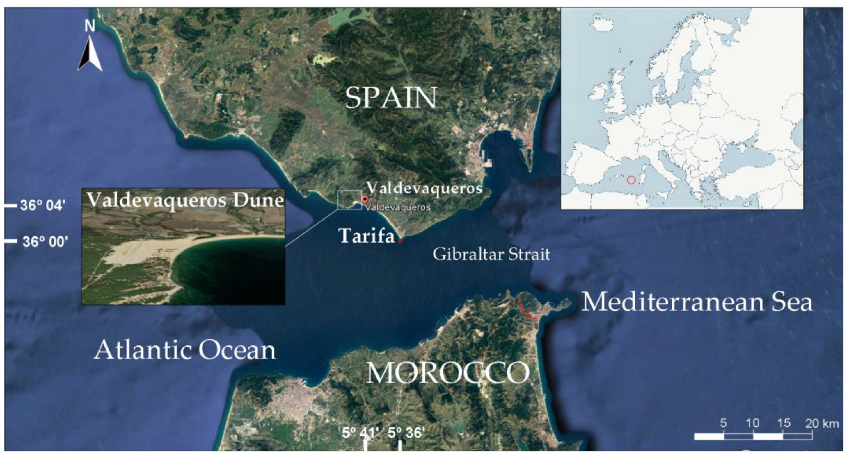
The study area is a coastal dune located in Valdevaqueros (Cadiz) on the southernmost point of Spain (Gibraltar Strait). The base data are meteorological data from Tarifa (Cádiz) and a 2012 field experiment carried out at the dune. The Valdevaqueros Dune (Cádiz) is approximately 10 km away from the meteorological station of Tarifa. The meteorological station of Tarifa is located on a promontory above the port basin and is managed by the Spanish Official Meteorology Agency (AEMET, www.aemet.es, accessed on 16 April 2023). The elevation (altitude) of the ground level at the Tarifa station is around 32.00 m above mean sea level (a.m.s.l.), which is used as a vertical datum for this research. Figure 1 illustrates the study site and shows the relative location of the meteorological station of Tarifa and the Valdevaqueros Dune.

This dune is in one of the windiest points in Spain. The system is formed by accumulations of sand that migrate from the beach due to intense easterly winds. The result is a sand formation oriented to the NE-SW, as Figure 2a,b show. Its dynamic is causing a relevant impact from a scientific and social point of view [19]. Here, the frequent occurrence of easterly winds has generated a highly mobile dune [20]. High sand migration rates occur in the dune because 70% of the wind speed exceeds the threshold velocity for sediment. The climatic conditions are unique for this area [21], mainly due to the presence of a long shoreline (more than 40 kilometers) and a cove before reaching the dune. This stretch of shoreline is only interrupted when the lagoon of the Valle River connects with the sea during the great floods [20]. The wind-blown sediment is a well-graded material composed mainly of quartz, with an average sand size of 0.3 mm [21,22].

The chosen study area is the Valdevaqueros Dune because it experiences a displacement of up to 1 m per day due to the eastern wind. The existence of a weather station (Tarifa) close to the dune and a predominant wind component from the weather station to the dune made us consider this place suitable for developing the methodology to propagate the wind from one point to another. Last, the dune advance is quick, and the sands are constantly invading the only road that connects to the rural settlement of Punta Paloma [23,24,25], as shown in Figure 2c. This transfer equation intends to be an additional tool in understanding how the movement is produced.

3. Materials and Methods

3.1. Methodology

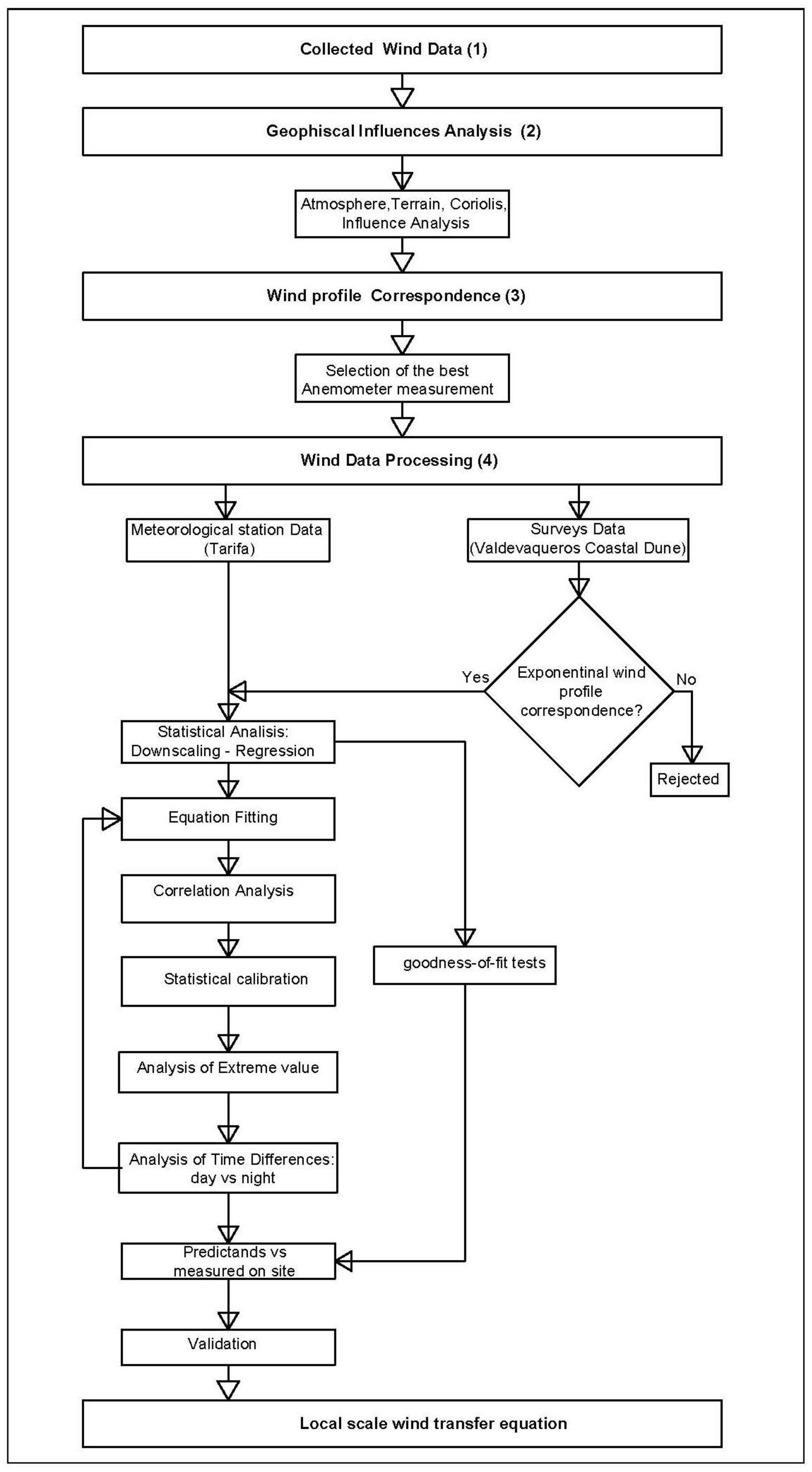
Data processing was established according to SD based on regression in order to obtain an equation for determining wind transfer between the Tarifa station and the dune. We also sought an accurate and tractable mathematical form.

3.1.1. Wind Data Processing

The first action was to check the difference between the samples and identify if they belonged to the same population (parts from the same group with the same features). For this goal, we used the Kruskal–Wallis (K-W) [26] (median test) and Mann–Whitney (M-W) tests [27,28]. Additionally, an analysis of variance (ANOVA) test [29] was applied to determine the strength of the relationship between the variables. There was a significant relationship between samples from both measurements when the uncertainty (p-value) was less than 5%. Otherwise, the samples were considered independent. The confidence level was 95%.

The next step consisted of searching for the type of regression that fit the transfer functions with the maximum correspondence between the predictors (velocities from Tarifa Station) and the predictands (velocities from the Valdevaqueros Dune).

All tests were carried out using the version 19.4.02 of Statgraphics Centurion software (Statgraphics Technologies, Inc., The Plains, VA, USA). The flow diagram in Figure 3 summarizes the proposed methodology.

3.1.2. Collected Wind Data

The present methodology is focused on a comparison of wind time series at the Tarifa meteorological station (Cadiz) (predictors) along with the record of a field experiment carried out at the Valdevaqueros Dune (Cadiz) in 2012 (predictands).

Table 1. Number of records per device and location.

Date	Year	Location	Elevation (Meters a.m.s.l)	Number of Records
March	2012	Tarifa (Met. Station)	32.00	16,210
October	2012	Tarifa (Met. Station)	32.00	17,847
6–27 March	2012	Valdevaqueros Dune	1.75	1286
6–27 March	2012	Valdevaqueros Dune	2.00	1286
6–27 March	2012	Valdevaqueros Dune	2.50	1286
6–27 March	2012	Valdevaqueros Dune	5.50	1286
1–23 October	2012	Valdevaqueros Dune	1.75	2468
1–23 October	2012	Valdevaqueros Dune	2.00	2468
1–23 October	2012	Valdevaqueros Dune	2.50	2468
1–23 October	2012	Valdevaqueros Dune	5.50	2468

shows the amount of processed data. The term “elevation” used below indicates the vertical distance from the anemometer to the mean sea level.

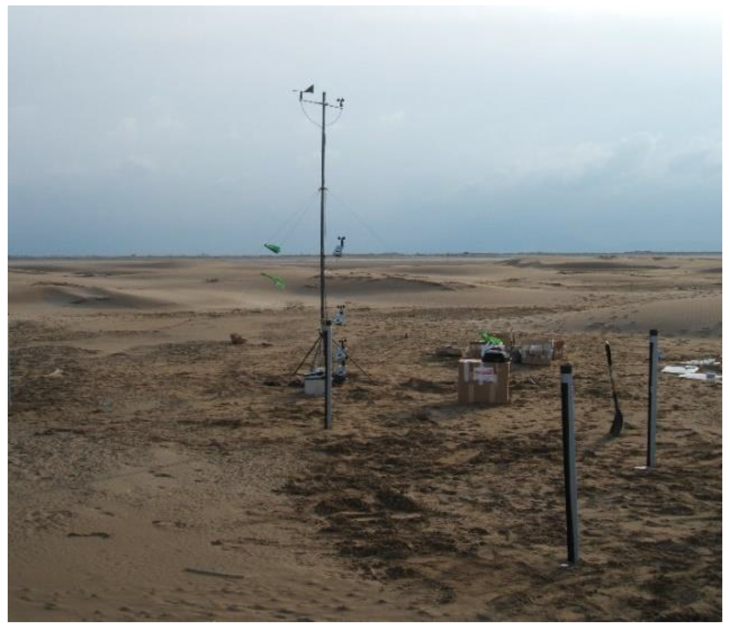
The field experiment carried out in 2012 measured wind data using a mast with anemometers at different heights of 0.25, 0.50, 1.00, and 4.00 m. Figure 4 shows the anemometer after being assembled on the windward part of the coastal dune (shoreline).

The elevation of the ground level where the anemometer mast was assembled was around 1.5 m a.m.s.l.

Table 2. Elevation of the assembled anemometers above ground level and above mean sea level.

Height of Anemometer Above Ground Level (m)	Elevation (Meters a.m.s.l)
0.25 m anemometers height	1.75 m
0.50 m anemometers height	2.00 m
1.00 m anemometers height	2.50 m
4.00 m anemometers height	5.50 m

shows the height of anemometers above the ground level and their corresponding elevation in meters above mean sea level:

The main features of the anemometers are included in

Table 3. Specification of assembled anemometers.

Model:	RM Young Model 03101
Range:	0 to 50 m s−1 (112 mph), gust survival 60 m s−1 (134 mph)
Sensor:	12 cm diameter cup wheel assembly, 40 mm diameter hemispherical cups
Accuracy:	±0.5 m s−1 (1.1 mph)
Threshold:	0.5 m s−1 (1.1 mph)

.

These anemometers registered data from the wind (velocity and direction) each minute during the months of March and October in 2012. The data were recorded each minute. All collected data were treated and used; however, due to the large quantity of these data, they are not included in the text to avoid disturbing the aim of this paper.

The time series data from the Tarifa station were provided by AEMET. These wind data from Tarifa Station (currently operational) were collected in ten-minute intervals, providing velocity values and angles for the direction of wind measured at this location.

Table 4. Data from the Tarifa weather station. Source: AEMET.

Network Code Indicator	Weather Name	Region	Town	Elevation (m)	Latitude	Longitude	Synoptical Indicative
6001	Tarifa	Cadiz	Tarifa	32	36°0′50″ N	5°35′56″ W	8458

shows the geographic features of the Tarifa Weather Station.

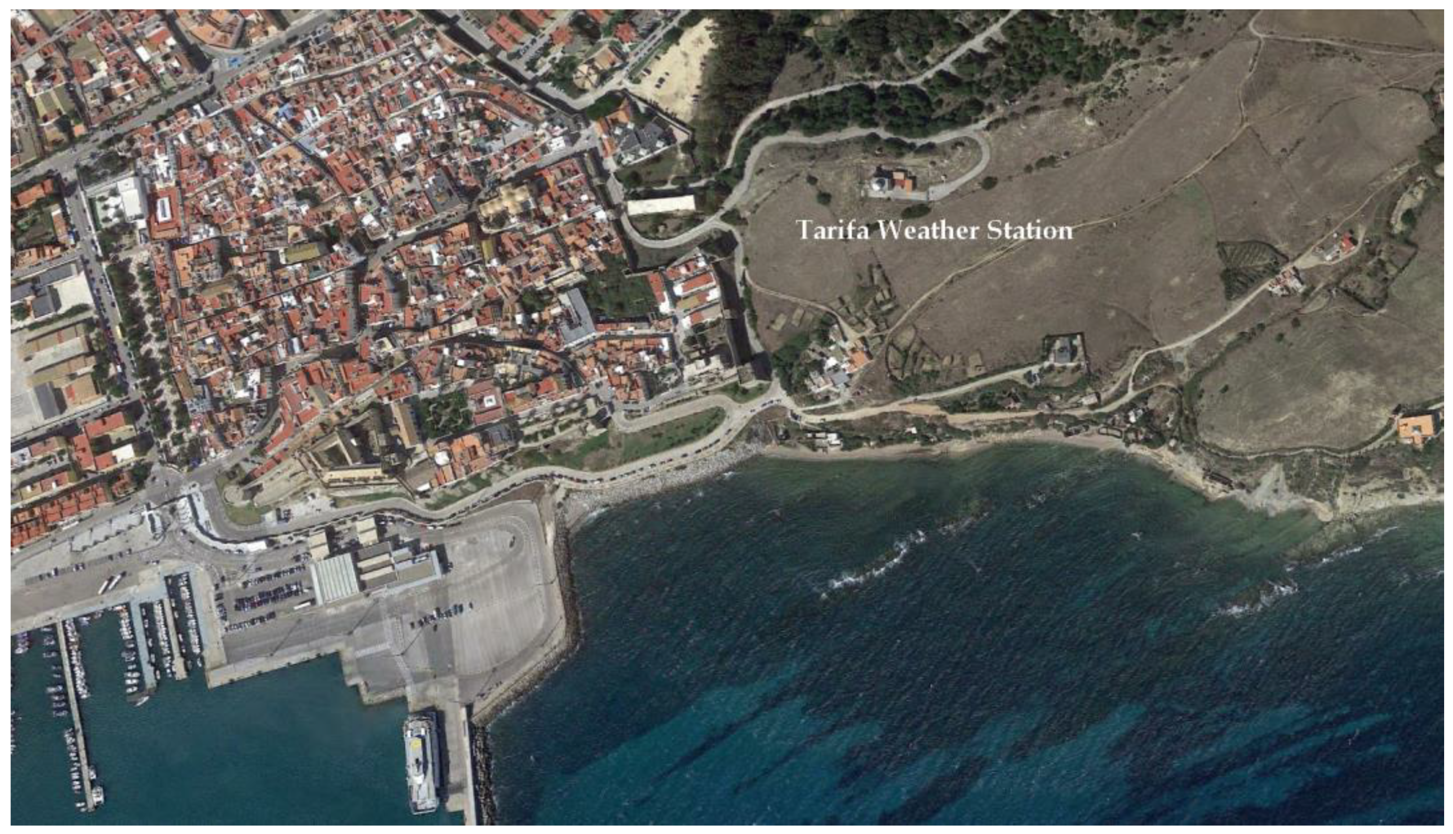
The elevation of the Tarifa anemometer is 10 m above the existing ground, which corresponds to 42 m. Figure 5 shows the location of the weather station.

In order to outline the wind behaviors at Tarifa Station,

Table 5. Comparative average data from Tarifa. Period 2010–2012.

Year	2010			2011			2012
Month	Average Speed (m/s)	Average Direction		Average Speed (m/s)	Average Direction		Average Speed (m/s)	Average Direction
January	5.72	177 º	S	5.49	159 º	SSE	4.59	145 º	SE
February	5.69	174 º	S	4.58	180 º	S	4.59	160 º	SSE
March	6.37	169 º	S	6.18	152 º	SSE	6.59	160 º	SSE
April	7.00	145 º	SE	7.63	143 º	SE	5.00	271 º	W
May	5.51	180 º	S	6.71	151 º	SSE	6.25	173 º	S
June	4.45	213 º	SSW	6.23	180 º	S	5.52	214 º	SW
July	6.80	150 º	SSE	5.36	209 º	SSW	5.87	204 º	SSW
August	6.35	126 º	SE	5.96	225 º	SW	5.36	222 º	SW
September	5.71	161 º	SSE	6.59	171 º	S	5.58	187 º	S
October	5.44	182 º	S	8.29	111 º	ESE	4.77	182 º	S
November	4.47	214 º	SW	4.69	162 º	SSE	4.46	173 º	S
December	6.16	150 º	SSE	3.93	199 º	SSW	3.71	206 º	SSW

shows the average speed and direction of wind for the period from 2010 to 2012. The table was elaborated from the data provided by AEMET. We can see that the variation in both average speed and average direction is very little.

3.1.3. Wind Profile Validation: Orographic Influence Analysis

The influence of the surrounding terrain and atmosphere was disregarded because the anemometers were placed only a few meters above sea level, and there were no significant landforms to consider [30,31,32,33]. The effects of these two factors could predetermine the intensity and acceleration of the winds in the area. First, the topography (rough terrain or complex orography) could produce an acceleration, and valleys yield a decrease in wind velocity [34]. However, in this case, both the dune and the meteorological station are located on points along the shoreline separated by 10 km, with no significant topography or sharp valley formations. The effects of the atmospheric gradient between the two points were found to be negligible at the shoreline [35]. Moreover, according to Barcons et al. (2018) [34], the Monin–Obukhov similarity theory [36] can be used to establish when the atmosphere has an influence. The relationship between the height (Z) and Obukhov length (L) [13] indicates when the atmosphere is stable, unstable, or neutral. The study area can be considered to have a neutral atmosphere with no effects on the winds.

Another physical law used in this study is the wind profile theory. This theory has been broadly used in research on the atmospheric boundary (within the surface layer) up to 100 m [37]. The investigation was carried out on the shoreline, and the wind profile power law is applicable up to 100 m height above the surface, so the application criterion is completely valid.

Finally, Coriolis acceleration is important for high scales with GCMs, but it was not included in our transfer function in a direct way due to the low roughness, flat terrain, and proximity of the two points in the study area. The roughness and terrain conditions are included in the power law, which is used to choose the best data. Overall, the local scale of the current study reduces the influence of orographic variables [38,39].

3.1.4. Wind Profile Correspondence

The following step evaluates the level of correspondence between both measurements. Here, we sought to determine if there was any relationship and how to compare the values. The wind profile power law was used to check which measurements from the field experiments in 2012 had the highest grade of correspondence with data from the Tarifa weather station. The selection of data from the anemometers consisted of determining the measurement that most closely approximated the wind profile. For the wind profile power law [17], we used Equation (1), frequently called the Hellman power law equation [18]. The logarithmic wind profile was also analyzed. However, this kind of profile is most suitable for wind power where the surface characteristics and the area have an important weight in the final expression [17,18].

$$Vz=Vref{\left(\frac{Z}{Zref}\right)}^{\alpha }$$

(1)

where Vz is the unknown velocity at the known elevation Z, Vref is the reference velocity at the known elevation Zref, and α is the wind shear coefficient for a certain area. The value for coefficient α is taken as 0.14; according to Rehman et al. (2015), this value is acceptable for heights up to 10 m [40] without introducing considerable deviations. The application of Equation (1) in this study aimed at verifying the anemometer height offering the best correspondence with the wind profile.

3.1.5. Day and Night Variation

As is generally the case, the wind blows stronger during the day than at night in the study area. Overall, wind speeds at Tarifa are always higher than the wind speeds in Valdevaqueros, independent of the time of the day. It has been observed that the variation in wind velocity is not so higher than 10 m/s between day and night. However, the directions have different behavior depending on if we are referring to the Tarifa station or the Valdevaqueros Dune. In the case of Tarifa, it is observed that the direction for the early hours of the morning is WNW. From 3 pm to 8 pm, approximately the main direction is ENE, and the rest of the day, ESE to S prevail as the main directions. This pattern practically remained constant both in winter and summer.

In the case of Valdevaqueros Dune, the directions behave differently between warm and cold seasons. In winter, it has been observed that the directions of WNW and NW are alternated as predominant throughout the day. On the other hand, in summer, the early hours of the morning start with NNE or NE winds, and they become ESE winds after noon to end the day, converted into SSE and S winds.

4. Results

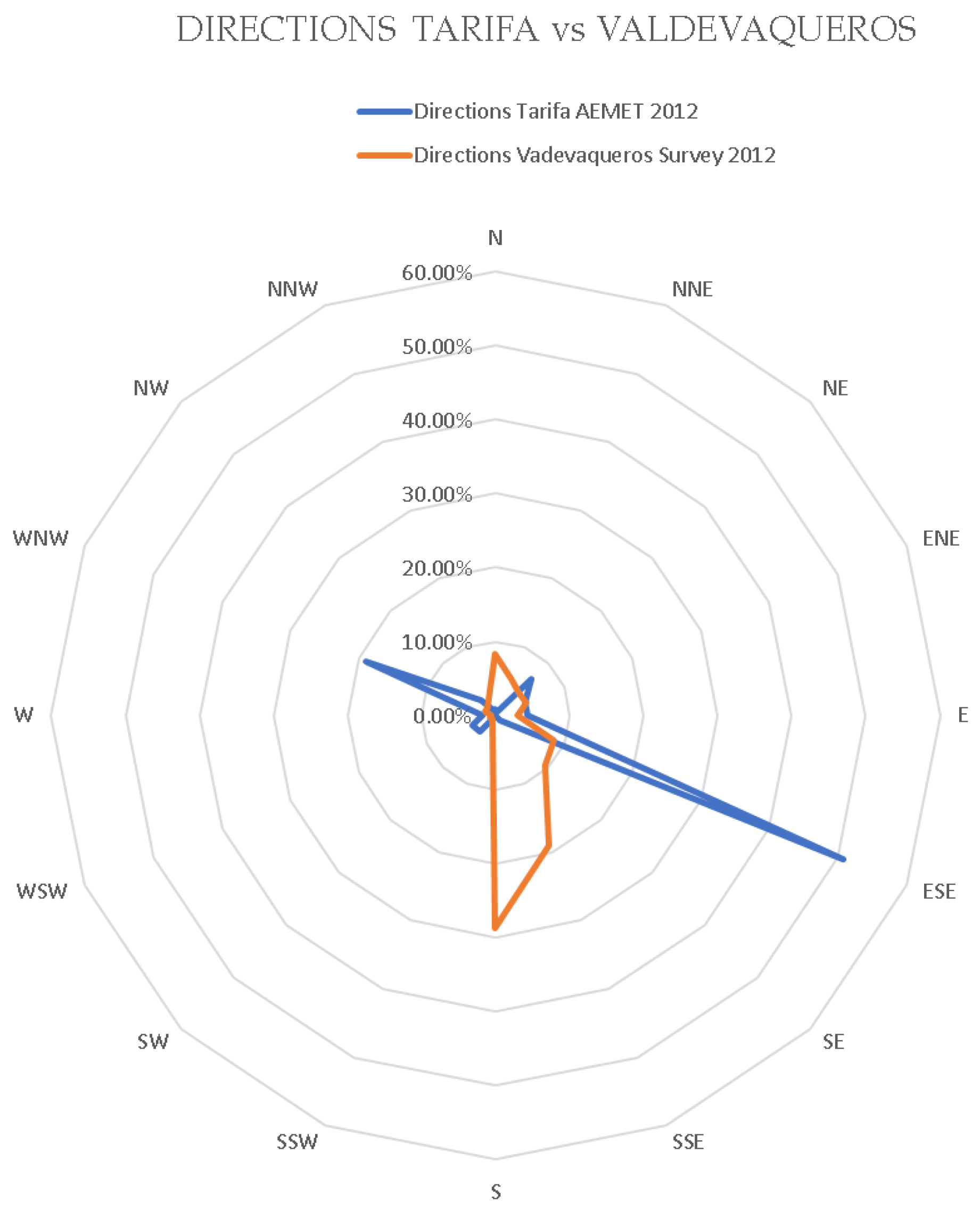
The data from the anemometers had to be processed and fitted with data from the meteorological station of Tarifa in order to align the correspondence between sampling frequencies. Figure 6 shows the different directions between the two measurements.

Before detailing the obtained results, we conducted a comparison between the collected data. The model has been trained (calibration) using the data from the field experiment carried out in March 2012, and it has been validated according to the data from the field experiment from October 2012.

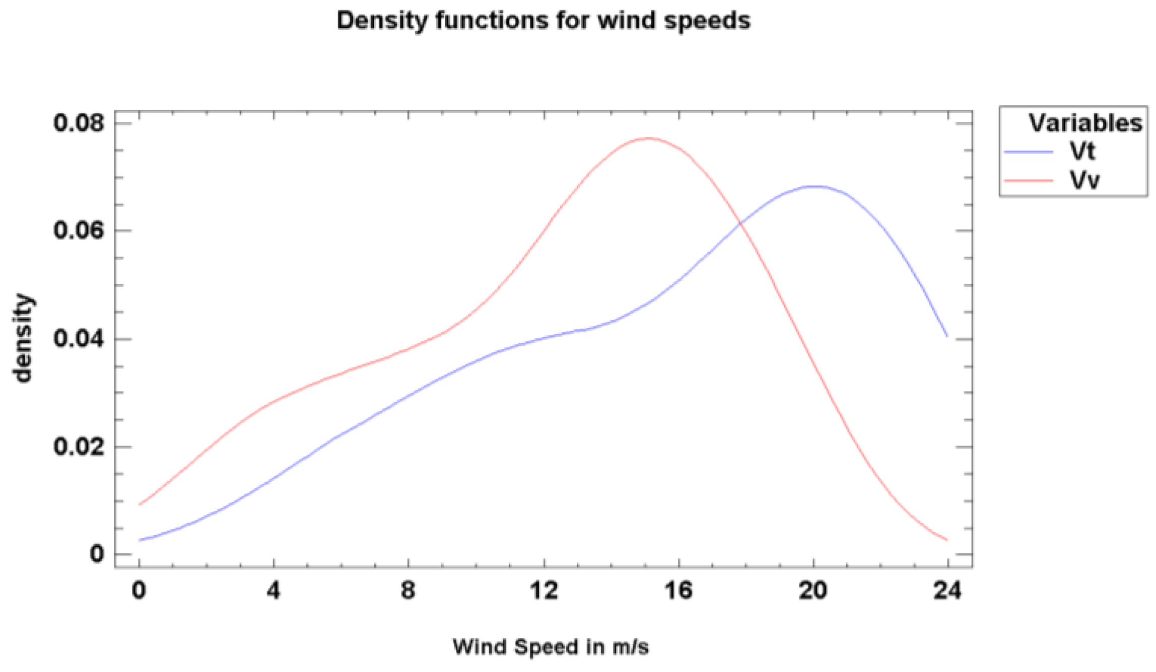
Figure 7 depicts the comparison between the two samples, where Vt is the wind velocity at Tarifa (predictors) station, and Vv is the wind velocity at Valdevaqueros Dune (predictands).

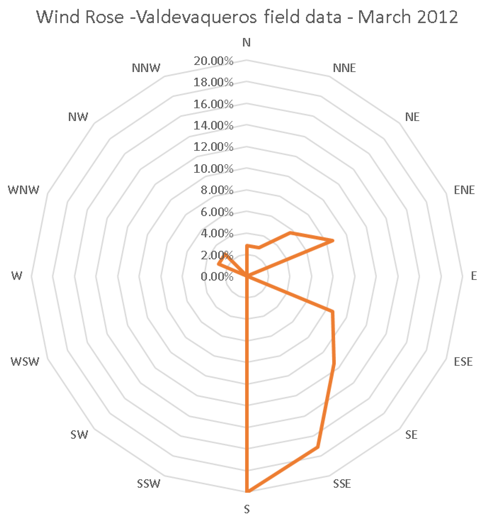
Regarding the wind directions, the values measured at Valdevaqueros indicated higher variability than those at Tarifa Station. Therefore, there is no main prevailing direction, but the east and south are the most representative directions overall. Figure 8 reflects the randomness of the directions measured at the coastal dune in March 2012.

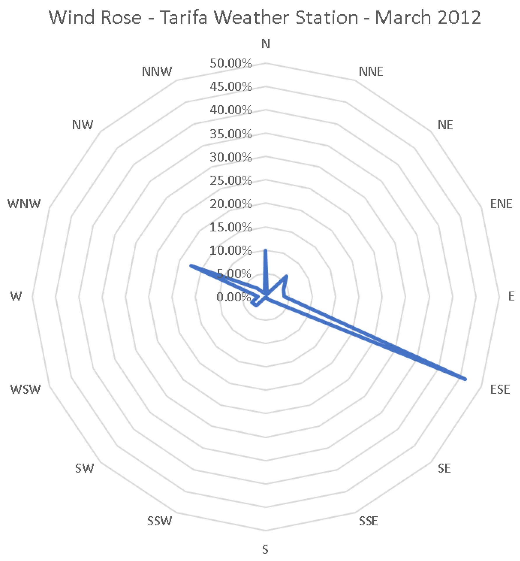
The prevailing direction at Tarifa is east–southeast, with a few variations turning around the north and west, which barely represent around 20% of the historical data. Figure 9 outlines the frequency of wind directions at Tarifa in March 2012.

East wind components predominate in the area, with a trend of changing wind from north to east–south. In both samples, the E–S wind component comprised 51% of the accounting records. The maximum values corresponded to the E–S direction, with higher values recorded for the ESE component. Figure 6 and Figure 7 show the changes in wind direction from Tarifa to Valdevaqueros because of the coast orientation.

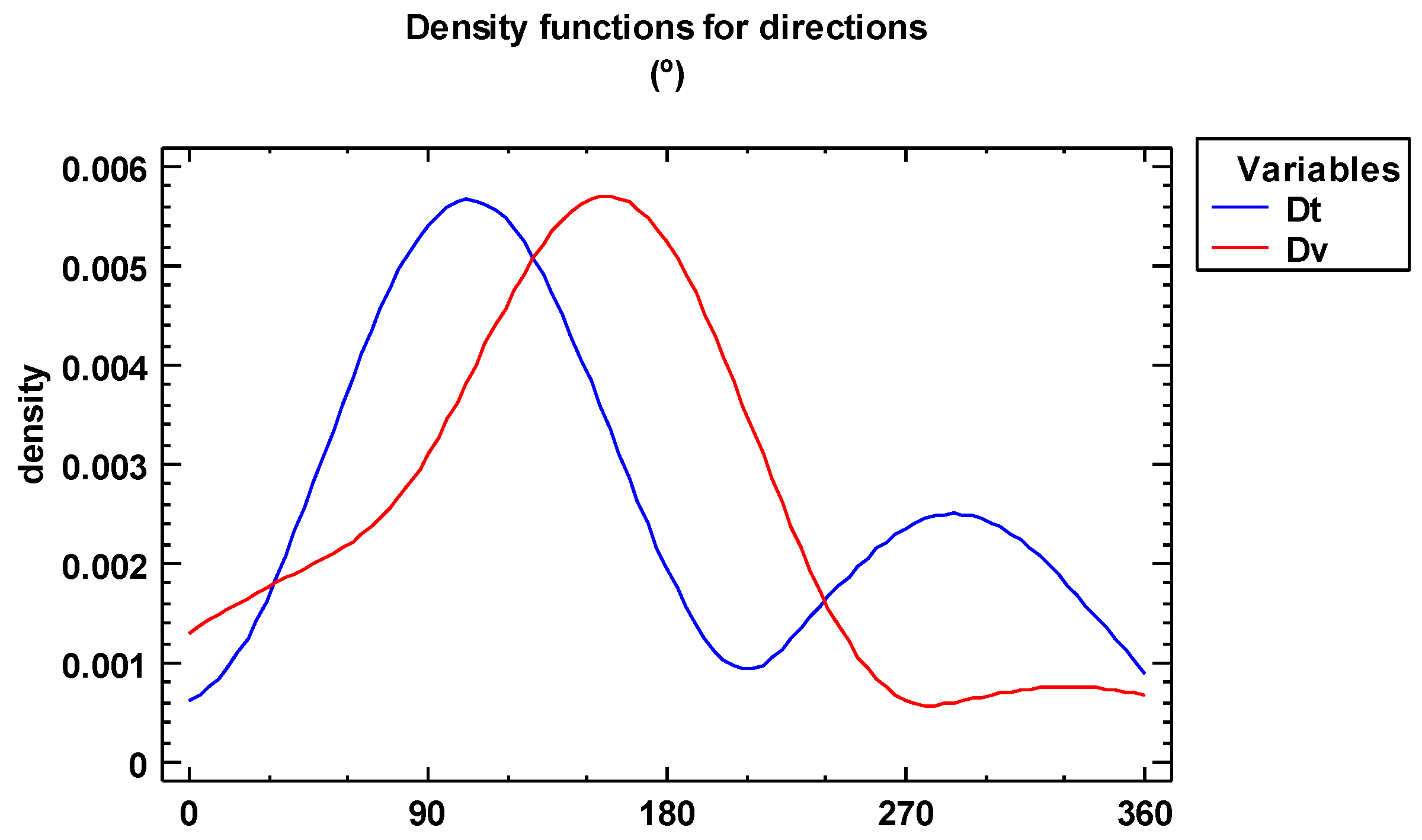
Figure 10 depicts the differences between the density traces of both samples, where Dt is the wind direction at the Tarifa (predictor) station, and Dv is the wind direction at Valdevaqueros Dune (predictand).

In a first approximation, we compared the anemometer data with the ones from the meteorological station of Tarifa. The aim was to determine the preliminary results obtained only by regression techniques without considering the power law application. Afterward, both outcomes, preliminary and final, were compared. The point here was to demonstrate that we can directly know which anemometer height fits better with the power law use. This saves an arduous, even difficult, process of fitting the data from each anemometer.

Table 6. Preliminary correlation (R) and determination (R²) coefficients: anemometers vs. Tarifa.

Vz	Correlation R	R2 (%)
V0.25	0.95	90.25
V0.50	0.91	82.81
V1.00	0.97	94.09
V4.00	0.91	82.81

shows the average correlation and determination coefficients for different regression models in an exploratory stage.

According to the methodology proposed above, two equations were used to correlate data from the two locations. These functions established the relationship between the speeds and directions of the winds measured at the Valdevaqueros Coastal Dune and the Tarifa meteorological station. The procedure to obtain the equations was SD. Specifically, we used downscaling based on regression [41].

A regression study was conducted using Equation (1) to obtain the best fit between the wind profile and the anemometer measurements. We took the values from the anemometer as a reference, and we applied the wind profile law. After that, we compared the results with data from the Tarifa station. The aim was to choose the best measurement to compare against data from Tarifa and thereby obtain equations with maximum accuracy.

Table 7. Correlation (R) and determination (R²) coefficients: wind profile results vs. Tarifa.

V0.25		V0.50		V1.00		V4.00
R	R2 (%)	R	R2 (%)	R	R2 (%)	R	R2 (%)
0.95	91.00	0.92	85.00	0.97	94.00	0.96	93.00

shows the correlation coefficient (R) and determination coefficient (R²) for both locations.

Comparing Table 6 and Table 7, we can show that by applying wind power law, we directly obtain the same results as we achieved with a hard regression process.

The previous table indicates that the data measured at a 1.00 m height have a better correspondence with the values obtained via the Hellman equation. Additionally, the regression study indicates that measurements at this height provide the best results.

Once we determined that the data from the anemometer assembled at 1.00 m in the Valdevaqueros Dune had the best regression coefficients, we began the process of realizing the transfer equations. The results are outlined in three subsections, one for the speeds, the other for directions, and a subsection for the validation of the model.

4.1. Transfer Function for Wind Speeds

As indicated in the methodology, although the logarithmic profile also fits well, the wind profile power law was superior, with higher accuracy and a better correlation for this location, as the area did not play an important role in this study because the wind fields are given from Tarifa weather station, and the aim was to obtain the best correspondence between data. For other sites, multiple assessments should be performed to choose the best profile. In this case, the surrounding area was deemed unimportant for the transference of wind since this parameter does not intervene in any case.

The results for the tests of K-W and M-W (0.23 and 0.18, respectively) allowed us to ensure that there was no significant difference between the medians of velocity from the anemometer measurements and the data from Tarifa.

Linear regression [42] was used to obtain the expression for the predictors and predictands. In the ANOVA test, high percentages were obtained for the correlation with the velocity.

Table 8. Correlation percentage for linear models of the velocity equation.

Model	Correlation	R-Squared
Multiplicative: Vv = exp(−0.97 + 1.25·ln(Vt))	0.99	97.57%
Double square root: Vv = (−0.54 + 1.01·√Vt)2	0.98	96.94%
Linear: Vv = −1.34 + 0.86·Vt	0.98	96.08%
Square root-X: Vv = −11.34 + 6.06·√Vt	0.98	95.08%

shows the correlation values for linear models with percentages above 95%.

In light of the results, we selected our model based on two goals: (1) obtaining the most accurate fitting and (2) obtaining a tractable mathematical expression. For this purpose, we selected the double square root model (Y = (a + b·√x)²).

Thus, the transfer equation to propagate the wind speeds from Tarifa Station to Valdevaqueros Dune was constructed via linear regression after transforming to a logarithmic scale to linearize the model by least squares fitting:

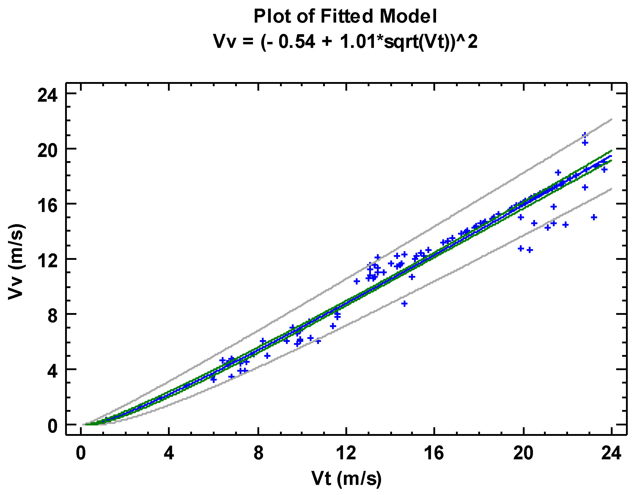
$$Vv={(-0.54+1.01·\sqrt{Vt})}^2$$

(2)

where Vv is the predictand for the velocity at the dune and Vt is the predictor (values measured at the meteorological station of Tarifa) with the coefficients in m/s. The ANOVA test yielded a value lower than 0.05 for fitting the coefficients a (−0.54) and b (1.01). The R-squared result indicated that the chosen model could explain 96.98% of the variability in speed. The correlation coefficient was 0.98, indicating a strong relationship between the variables. The standard error of estimations is 0.14, and the mean absolute error is 0.09. These results demonstrate that the methodology presented here can obtain a highly accurate mathematical expression. Figure 11 provides a graph illustrating the values resulting from Equation (2).

The gray lines indicate the confidence range (95%); this is the range of values that we expect the predictands to fall. The green lines indicate the prediction limits (95%), the range of values that will likely contain a future prediction. The confidence range and prediction limits are computed using the mean and standard deviation, mean squared error (MSE), and the critical values for the statistical test applying normal distribution [43,44,45]. Equations (3) and (4) show the general expression of a confidence range:

$$CR=\overline{x}\mp Z·\left(\frac{s}{\sqrt{n}}\right)$$

(3)

$$PL=P(-z<Z<z)$$

(4)

where CR is the confidence range, PL is the prediction limits, $\overline{x}$ is the sample mean, Z is the critical value of the z distribution, s is the sample standard deviation, n is the sample size, and z is the corresponding quantile of the normal distribution.

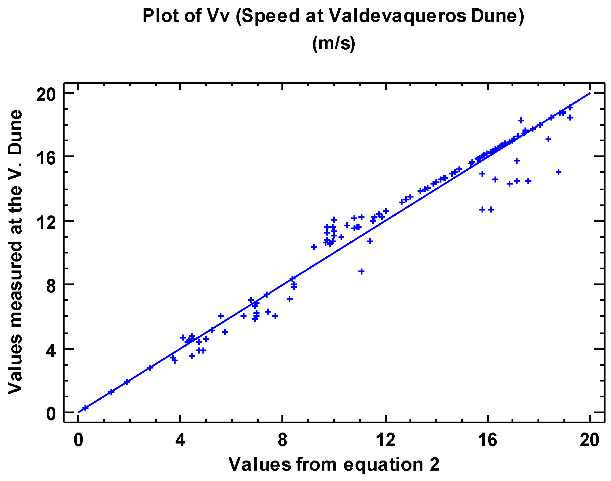
Finally, we carried out an analysis of the results. The values from the equation were compared with the values from the field experiments (data from the anemometer placed at a 1.00 m height). To evaluate the model, we used the leverage parameter [46]. This parameter measures how influential each observation is in determining the coefficients of the estimated model. In this case, an average data point would have a leverage value equal to 0.015. This indicates that there are no important deviations from the measured data from the dune. Figure 12 illustrates this comparison.

4.2. Transfer Function for Wind Directions

The process to obtain the transfer function for directions is the same as that used for the speed values in Section 4.1; to avoid repetition of the mathematical steps, a summary of the design criteria, input data, and the results are provided.

The function lets us know the wind direction in Valdevaqueros with previous data from Tarifa. This is the propagation of wind direction data from Tarifa, but only those that reach Valdevaqueros. This implies that this equation is only able to transfer data in those directions, from the Tarifa to Valdevaqueros, and not the other way around. Thus, the equations provide data for the directions input from ENE to SSE, being this the wind directions that reach Valdevaqueros from Tarifa. This feature of the function is aligned with these directions, corresponding to the maximum speed, and they produce the maximum movement in the dune.

Table 9. Adjusted data input for wind direction transfer function.

Location:	TARIFA		VALDEVAQUEROS
Date:	Dt		Dv
…	…	…	…	…
7 March 2012 14:50:00	118	ESE	132	SE
7 March 2012 15:00:00	117	ESE	131	SE
7 March 2012 15:10:00	113	ESE	128	SE
7 March 2012 15:20:00	112	ESE	127	SE
…	…	…	…	…
27 March 2012 13:40:00	114	ESE	129	SE
27 March 2012 13:50:00	115	ESE	130	SE
…	…	…	…	…

shows an example of the average directions taken every 10 min, used to determine the direction transfer function.

Inference for regression is applied due to its usability. Correspondence between directions requires a different type of regression than the linear type. For the directions, the correlation is not as direct as that of the velocities. This variability is shown in Figure 5 (wind roses comparative).

After different linear and polynomial regression trials, the best way to fit the relationship was determined to be orthogonal regression [47,48,49,50,51]. The main difference between the least squares, used for speeds, and the orthogonal regressions, for directions, is the way to minimize the distance to the fitted line (vertical in the first one and perpendicular in the second one).

Table 10. Comparison of alternative models for wind directions.

Model	Correlation
Double Reciprocal: Dv = 1/(0.001 + 0.73/Dt)	0.98
Multiplicative: Dv = exp(0.99 + 0.81·ln(Dt))	0.98
Square root-Y logarithmic-X: Dv = (−11.28 + 4.78·ln(Dt)) ^ 2	0.98
Square root-X:Dv = −88.05 + 20.29·√Dt	0.98

shows the correlation values for orthogonal regression models with percentages above 95%.

This analysis is identical to that presented in the previous paragraph. Equation (5) is based on the same model as Equation (2) (Y= (a + b·√x)²):

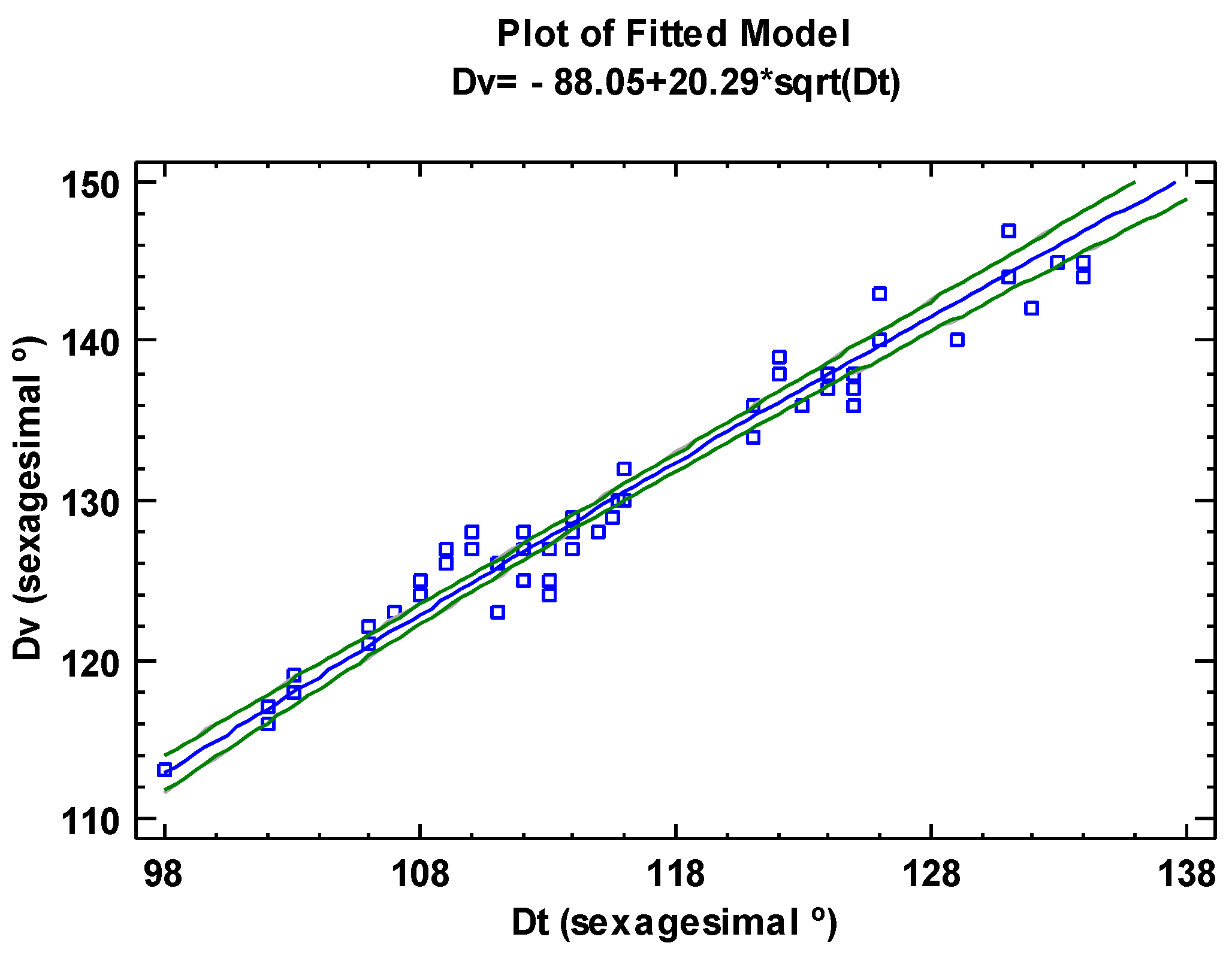
$$Dv=(-88.05+20.29·\sqrt{Dt})$$

(5)

where Dv is the predictand for the direction at the dune, and Dt is the predictor (measured values from the meteorological station of Tarifa). Both are expressed in sexagesimal degrees (°).

Table 11. Error of the coefficients for wind directions function.

Parameter	Orthogonal Estimate	Standard Error
Intercept	−88.0558	6.51
Slope	20.2943	0.60

shows the error for the coefficients:

Figure 13 graphs the resulting values from Equation (5). The gray lines indicate the confidence ranges (95%), and the green lines indicate the prediction limits.

4.3. Model Validation

As indicated in the previous paragraph, the model has been trained with the data from the field experiment carried out in March 2012. In order to validate the achieved transfer functions, data from the field experiment carried out in October 2012 has been randomly chosen to check the models.

Table 12. Model validation results. Vt₀, Dt₀ (registered data in Tarifa) and Vv₀, Dv₀ (registered data in Valdevaqueros).

	Registered Data				Propagated Wind Data
	Tarifa Meteorological Station		Valdevaqueros Dune—Anemometer 1.0 Height		Valdevaqueros Dune
Date	Vt0 (m/s)	Dt0 (º)	Vv0 (m/s)	Dv0 (º)	Vv (m/s)	Dv (º)	Vv Error (%)	Dv Error(%)
2 October 2012 14:00:00	6.9	115	4.88	132	4.49	137	8.0	3.9
2 October 2012 14:30:00	8.5	116	5.33	121	5.81	138	9.0	13.8
2 October 2012 15:20:00	7.9	116	5.67	128	5.31	138	6.3	7.5
2 October 2012 16:20:00	7.5	116	4.71	121	4.98	138	5.7	14.2
2 October 2012 17:10:00	6.5	116	4.13	133	4.16	138	0.8	3.9
2 October 2012 18:10:00	6.6	116	4.15	128	4.24	138	2.3	7.5
3 October 2012 12:10:00	9.7	117	6.8	133	6.82	139	0.2	4.8
3 October 2012 13:20:00	8.8	115	6.12	129	6.06	137	0.97	6.2
3 October 2012 14:10:00	8.6	115	5.94	131	5.89	137	0.79	4.7
						Average Error (%)	3.8	5.0

shows the results and the error with respect to the measurement. The directions have been checked only for the direction in Tarifa, which take relevance in Valdevaqueros (ESE-SSE).

As the data were collected each minute at the dune and every 10 min in Tarifa Station, the input data in Table 12 are the average of the corresponding 10 values for the Valdevaqueros Dune. This is the way to compare data in the same conditions. The average error for speeds and directions is around 4% and 5%, respectively, removing the outliers.

5. Discussion

Based on the above equations and their results, although the fitting provided a high correlation, the calibration process should continue in future work. The field experiment data were enough for developing the methodology and testing the model, but it is necessary to carry out new data collection on site. This will be performed in future works with the double aim of ensuring the representativeness and resilience of the equations against the unsteady atmospheric processes. This would also greatly increase the validity of the developed function, as it would potentially show that the data used for March and October 2012 were similar over several years. However, this trend is shown in Table 5 for the period from 2012 to 2013. In addition, this future work will compare the obtained results by our spatial transfer functions with the GCMs, especially with the COSMO-REA6 hindcast. This GCM is chosen because it is a reanalysis system that operates with dataset features a 6 × 6 km horizontal resolution from 1995 to 2019. This comparison is geared to cross-check against the results from both transfer equations and GCMs at a local scale. The aim is to verify and/or improve our functions as well as validate the accuracy of GCMs in this regard.

One further point to be studied is the splitting of the transfer function for velocities in stretches covering different ranges of data. An open hypothesis is whether one can obtain a function for the medium values and another for the extreme values in order to further improve the current results. The same question could be applied to directions far from the predominant direction (ESE), although such directions represent less than 10% of the sample. In this case, we could split the equation into three stretches, as proposed for the modules, with one for the N-E range, another for E-W, and the last for W-N. Placing the focus on the prevailing wind direction rather than the other directions has facilitated the search for relevant equations.

It is also important to remark upon the high values of these coefficients. The core element was the introduction of the wind profiles in the investigation.

6. Conclusions

This paper aimed at resolving the lack of methods, using a relatively simple technique, for wind transference/propagation at a local scale. Most local predictions are based on GCMs, but their design is suitable for global weather forecasting and climate change. However, GCMs can be run at a local scale, but they need a huge amount of data for reanalysis and assumptions that sometimes may lead to more uncertainties and limitations of the results at this spatial resolution. SD is increasingly applied to develop local climate information from the GCM resolution. This work explores the way to carry out wind propagation based on locations with wind serial data information not further than 10 km.

The proposed method is based on a comparison between the power law and data collected on site. This led us to select the most suitable wind data between 4 anemometers assembled at different heights from a field experiment. These data were then matched with data from a nearby weather station. The area is influenced by a strong eastern wind component.

Another important aspect of this investigation was the application of the power law (wind profile) to select the best data from the field experiment. This process indicated that data from the anemometer assembled at a 1.0 m height were better to compare against data from the station of Tarifa. This means the functions to propagate (transfer) winds have been developed considering the data from Tarifa and the anemometer at 1.0 m height.

After analyzing the methodology and its results, we found that the achieved transfer functions allowed us to determine the winds acting on the coastal dune of Valdevaqueros, for speeds and direction from ENE-SE, with an average error under 5%.

In the end, high correlation values confirmed a suitable fit between the data. The accuracy of the equations was also high according to the R values (≈0.98) for both velocities and directions.

Finally, this methodology should be feedback with new data from longer field experiments and evaluated on other sites in order to obtain the physical interpretation of the parameters of the transfer functions beyond the mathematical sense and continue improving the fit. Furthermore, future works will be carried out to check GCMs versus these transfer functions in order to improve the proposed local model and explore the possibilities joined with GCMs.

References

1. Wilby, R.; Wigley, T. Downscaling general circulation model output: A review of methods and limitations. Prog. Phys. Geogr. Earth Environ. 1997, 21, 530–548. [Google Scholar] [CrossRef]
2. Gutiérrez, J.M.; San-Martín, D.; Brands, S.; Manzanas, R.; Herrera, S. Reassessing Statistical Downscaling Techniques for Their Robust Application under Climate Change Conditions. J. Clim. 2013, 26, 171–188. [Google Scholar] [CrossRef]
3. Pielke, R.A.; Wilby, R.L. Regional climate downscaling: What’s the point? Eos Trans. Am. Geophys. Union 2012, 93, 52–53. [Google Scholar] [CrossRef]
4. Devis, A.; Van Lipzig, N.P.M.; Demuzere, M. A new statistical approach to downscale wind speed distributions at a site in northern Europe. J. Geophys. Res. Atmos. 2013, 118, 2272–2283. [Google Scholar] [CrossRef]
5. Bettolli, M. Analog Models for Empirical-Statistical Downscaling. In Oxford Research Encyclopedia of Climate Science; Oxford University Press: Oxford, UK, 2021. [Google Scholar] [CrossRef]
6. Urraca, R.; Huld, T.; Gracia-Amillo, A.; Martinez-de-Pison, F.J.; Kaspar, F.; Sanz-Garcia, A. Evaluation of global horizontal irradiance estimates from ERA5 and COSMO-REA6 reanalyses using ground and satellite-based data. Sol. Energy 2018, 164, 339–354. [Google Scholar] [CrossRef]
7. Bollmeyer, C.; Keller, J.D.; Ohlwein, C.; Wahl, S.; Crewell, S.; Friederichs, P.; Hense, A.; Keune, J.; Kneifel, S.; Pscheidt, I.; et al. Towards a high-resolution regional reanalysis for the european CORDEX domain. Q. J. R. Meteorol. Soc. 2015, 141, 686. [Google Scholar] [CrossRef]
8. Marzban, C.; Sandgathe, S.; Kalnay, E. MOS, Perfect Prog, and Reanalysis. Mon. Weather. Rev. 2006, 134, 657–663. [Google Scholar] [CrossRef]
9. Eden, J.M.; Widmann, M.; Grawe, D.; Rast, S. Skill, Correction, and Downscaling of GCM-Simulated Precipitation. J. Clim. 2012, 25, 3970–3984. [Google Scholar] [CrossRef]
10. Gómez Lahoz, M.; Albiach, J.C.C. Wave forecasting at the Spanish coasts. J. Atmos. Ocean Sci. 2005, 10, 389–405. [Google Scholar] [CrossRef]
11. Vidal, J.; Berrocoso, M.; Jigena, B. Hydrodynamic Modeling of Port Foster, Deception Island (Antarctica). In Nonlinear and Complex Dynamics; Machado, J.A.T., Baleanu, D., Luo, A.C.J., Eds.; Springer: London, UK, 2011. [Google Scholar]
12. Jigena, B.; Berrocoso, M.; Torrecillas, C.; Vidal, J.; Barbero, I.; Fernandez-Ros, A. Determination of an experimental geoid at Deception Island, South Shetland Islands, Antarctica. Antarct. Sci. 2016, 28, 277–292. [Google Scholar] [CrossRef]
13. Martinez-García, F.P.; Contreras-de-Villar, A.; Muñoz-Perez, J.J. Review of Wind Models at a Local Scale: Advantages and Disadvantages. J. Mar. Sci. Eng. 2021, 9, 318. [Google Scholar] [CrossRef]
14. Bauer, B.O.; Hesp, P.A.; Walker, I.J.; Davidson-Arnott, R.G. Sediment transport (dis)continuity across a beach-dune profile during an offshore wind event. Geomorphology 2015, 245, 135–148. [Google Scholar] [CrossRef]
15. Negro, V.; López-Gutiérrez, J.-S.; Esteban, M.D.; Alberdi, P.; Imaz, M.; Serraclara, J.-M. Monopiles in offshore wind: Preliminary estimate of main dimensions. Ocean Eng. 2017, 133, 253–261. [Google Scholar] [CrossRef]
16. Contreras-De-Villar, F.; García, F.J.; Muñoz-Perez, J.J.; Contreras-De-Villar, A.; Ruiz-Ortiz, V.; Lopez, P.; Garcia-López, S.; Jigena, B. Beach Leveling Using a Remotely Piloted Aircraft System (RPAS): Problems and Solutions. J. Mar. Sci. Eng. 2020, 9, 19. [Google Scholar] [CrossRef]
17. Bañuelos-Ruedas, F.; Angeles-Camacho, C.; Rios-Marcuello, S. Analysis and validation of the methodology used in the extrapolation of wind speed data at different heights. Renew. Sustain. Energy Rev. 2010, 14, 2383–2391. [Google Scholar] [CrossRef]
18. Gunda, L.; Chikuni, E.; Tazvinga, H.; Mudare, J. Estimating wind power generation capacity in Zimbabwe using vertical wind profile extrapolation techniques: A case study. J. Energy S. Afr. 2021, 32, 14–26. [Google Scholar] [CrossRef]
19. Bello-Millán, F.J.; Somoano, M.; Clavero, M.; Gómez-Pina, G.; Losada, M.A. El sistema dunar de Valdevaqueros: Evolución histórica y alternativas de gestión. Ribagua 2016, 3, 2. [Google Scholar] [CrossRef]
20. Toffani, M. Morphodynamic study of the dunes from Bahía Creek dunefield, Río Negro, Argentinian Patagonia. Latin Am. J. Sedimentol. Basin Anal. 2020, 27, 55–79. [Google Scholar]
21. Yue, Z.; Yuan, X.; Cao, L.; Tian, F.; Han, C.; Zhang, H. Characteristics and variation law of wind-blown sand delivered to the Ningxia–Inner Mongolia reach of the Yellow River under a changing environment. Int. J. Sediment Res. 2022, 37, 2. [Google Scholar] [CrossRef]
22. Muñoz-Perez, J.J.; Navarro, M.; Roman-Sierra, J.; Tejedor, B.; Rodriguez, I.; Gomez-Pina, G. Long-term evolution of a transgressive migrating dune using reconstruction of the EOF method. Geomorphology 2009, 112, 167–177. [Google Scholar] [CrossRef]
23. Fages-Antiñolo, L.; Gomez-Pina, G.; Navarro-Pons, M.; Román-Sierra, J.; Gimenez-Cuenca, M.; Ruiz, J.A.; Muñoz-Perez, J.J. Coastal Management Activities in Valdevaqueros Dune Area (Tarifa, SW Spain). In Proceedings of the International Conference on Management and Restoration of Coastal Dunes ICCD 2007, Santander, Spain, 27 September 2007; Universidad de Cantabria: Cantabria, Spain. [Google Scholar]
24. Gómez-Pina, G.; Fages-Antiñolo, L.; Ramírez, J.L.; Muñoz-Pérez, J.J.; Enríquez, J. A critical review of beach restoration projects in the northern coast of Cadiz (Spain) after thirteen years. Coast. Eng. 2006, 5, 4167–4178. [Google Scholar] [CrossRef]
25. Navarro-Pons, M.; Muñoz-Pérez, J.J.; Román-Sierra, J.; García, S. Evidence of coastal dune mobility increases over the last half century in response to historical human intervention. Sci. Mar. 2016, 80, 261–272. [Google Scholar] [CrossRef]
26. Ostertagová, E.; Ostertag, O.; Kováč, J. Methodology and Application of the Kruskal-Wallis Test. Appl. Mech. Mater. 2014, 611, 115–120. [Google Scholar] [CrossRef]
27. Gibbons, J.D.; Chakraborti, S. Nonparametric Statistical Inference. In International Encyclopedia of Statistical Science; Springer: Berlin/Heidelberg, Germany, 2010. [Google Scholar] [CrossRef]
28. Boudia, S.M.; Santos, J.A. Assessment of large-scale wind resource features in Algeria. Energy 2019, 189, 116299. [Google Scholar] [CrossRef]
29. Liu, H. Comparing Welch’s ANOVA, a Kruskal-Wallis test and traditional ANOVA in case of heterogeneity of variance ANOVA. Master’s Thesis, Virginia Commonwealth University, Richmond, VA, USA, 8 April 2015. [Google Scholar]
30. Ryu, G.H.; Kim, Y.G.; Kwak, S.J.; Choi, M.S.; Jeong, M.S.; Moon, C.J. Atmospheric Stability Effects on Offshore and Coastal Wind Resource Characteristics in South Korea for Developing Offshore Wind Farms. Energies 2022, 15, 1305. [Google Scholar] [CrossRef]
31. Barthelmie, R.J. The effects of atmospheric stability on coastal wind climates. Meteorol. Appl. 1999, 6, 39–47. [Google Scholar] [CrossRef]
32. Bardal, L.M.; Onstad, A.E.; Sætran, L.R.; Lund, J.A. Evaluation of methods for estimating atmospheric stability at two coastal sites. Wind. Eng. 2018, 42, 561–575. [Google Scholar] [CrossRef]
33. Wharton, S.; Lundquist, J. Atmospheric stability impacts on power curves of tall wind turbines—An analysis of a west coast north american wind farm. Environ. Res. Lett. 2010, 7, 014005. [Google Scholar] [CrossRef]
34. Barcons, J.; Avila, M.; Folch, A. A wind field downscaling strategy based on domain segmentation and transfer functions. Wind. Energy 2018, 21, 409–425. [Google Scholar] [CrossRef]
35. Fraile Jurado, P.; Aguilar Alba, M. La influencia de la presión atmosférica y el viento en la variabilidad del nivel del mar en el mareógrafo de Bonanza (Cádiz). In Proceedings of the Clima, Sociedad y Medio Ambiente, Zaragoza, Spain, May 2006. Asociacion Española de Climatologia, Spain. [Google Scholar]
36. Cheng, Y.; Zhang, M.; Zhang, Z.; Xu, J. A new analytical model for wind turbine wakes based on Monin-Obukhov similarity theory. Appl. Energy 2019, 239, 96–106. [Google Scholar] [CrossRef]
37. Guevara Díaz, J.M. Cuantificación del perfil del viento hasta 100 m de altura desde la superficie y su incidencia en la climatología eólica. Terra 2013, 29, 81–101. [Google Scholar]
38. Crosman, E.T.; Horel, J.D. Sea and Lake Breezes: A Review of Numerical Studies. Bound.-Layer Meteorol. 2010, 137, 1–29. [Google Scholar] [CrossRef]
39. Steele, C.J.; Dorling, S.R.; von Glasow, R.; Bacon, J. Idealized WRF model sensitivity simulations of sea breeze types and their effects on offshore windfields. Atmos. Chem. Phys. 2013, 13, 443–461. [Google Scholar] [CrossRef]
40. Rehman, S.; Shoaib, M.; Siddiqui, I.; Ahmed, F.; Tanveer, M.; Jilani, S.U. Effect of Wind Shear Coefficient for the Vertical Extrapolation of Wind Speed Data and its Impact on the Viability of Wind Energy Project. J. Basic Appl. Sci. 2015, 11, 90–100. [Google Scholar] [CrossRef]
41. Hewitson, B.C.; Daron, J.; Crane, R.G.; Zermoglio, M.F.; Jack, C. Interrogating empirical-statistical downscaling. Clim. Chang. 2014, 122, 539–554. [Google Scholar] [CrossRef]
42. Mao, Y.; Monahan, A. Linear and nonlinear regression prediction of surface wind components. Clim. Dyn. 2018, 51, 3291–3309. [Google Scholar] [CrossRef]
43. Lawless, J.F.; Fredette, M. Frequentist prediction intervals and predictive distributions. Biometrika 2005, 92, 3. [Google Scholar] [CrossRef]
44. Zeng, J.; Fletcher, D.; Dillingham, P.W.; Cornwall, C.E. Studentized bootstrap model-averaged tail area intervals. PLoS ONE 2019, 14, 3. [Google Scholar] [CrossRef]
45. Sedgwick, P. Understanding confidence intervals. BMJ 2014, 349, g6051. [Google Scholar] [CrossRef] [PubMed]
46. Everitt, B.S.; Skrondal, A. Review of The Cambridge Dictionary of Statistics, 4th ed.; Cambridge University Press: Cambridge, UK, 2006; pp. 247, 319, 422. [Google Scholar]
47. Wu, C.; Yu, J.Z. Evaluation of linear regression techniques for atmospheric applications: The importance of appropriate weighting. Atmos. Meas. Tech. 2018, 11, 1233–1250. [Google Scholar] [CrossRef]
48. Carr, J.R. Orthogonal regression: A teaching perspective. Int. J. Math. Educ. Sci. Technol. 2012, 43, 134–143. [Google Scholar] [CrossRef]
49. Leng, L.; Zhang, T.; Kleinman, L.; Zhu, W. Ordinary least square regression, orthogonal regression, geometric mean regression and their applications in aerosol science. J. Phys. Conf. Ser. 2007, 78, 012084. [Google Scholar] [CrossRef]
50. Carroll, R.J.; Ruppert, D. The Use and Misuse of Orthogonal Regression in Linear Errors-in-Variables Models. Am. Stat. 1996, 50, 1–6. [Google Scholar] [CrossRef]
51. Carreno-Madinabeitia, S.; Ibarra-Berastegi, G.; Sáenz, J.; Zorita, E.; Ulazia, A. Sensitivity Studies for a Hybrid Numerical–Statistical Short-Term Wind and Gust Forecast at Three Locations in the Basque Country (Spain). Atmosphere 2020, 11, 45. [Google Scholar] [CrossRef]
Figure 1. Site study location.
Jmse 11 00923 g001
Figure 2. Valdevaqueros Dune. (a) View from NW; (b) dune profile; (c) buried road by the dune.
Jmse 11 00923 g002
Figure 3. Methodology flow chart.
Jmse 11 00923 g003
Figure 4. Anemometers used at the Valdevaqueros Dune in 2012.
Jmse 11 00923 g004
Figure 5. Tarifa weather station location.
Jmse 11 00923 g005
Figure 6. Wind roses comparative: Valdevaqueros versus Tarifa.
Jmse 11 00923 g006
Figure 7. Comparative density functions for speeds (m/s) at both locations.
Jmse 11 00923 g007
Figure 8. Wind rose at Valdevaqueros—March 2012.
Jmse 11 00923 g008
Figure 9. Wind rose at Tarifa Station—March 2012.
Jmse 11 00923 g009
Figure 10. Density functions for directions in both locations.
Jmse 11 00923 g010
Figure 11. Plot of fitted model for speed.
Jmse 11 00923 g011
Figure 12. Plot of values from equation 2 vs. values measured on site for speed.
Jmse 11 00923 g012
Figure 13. Plot of the fitted model for directions. Dv (predictands from Valdevaqueros) and Dt (predictors from Tarifa).
Jmse 11 00923 g013