Hydrodynamics and Sediment-Transport Pathways along a Mixed-Energy Spit-Inlet System: A Modeling Study at Chincoteague Inlet (Virginia, USA)

Abstract

Tidal-inlet systems are dynamic features that respond to short-term (e.g., storms) and longer-term processes (e.g., sea-level rise, changes in tidal prism). The Chincoteague Inlet system, located along the northern Eastern Shore of Virginia (USA), is a dynamic coastal complex that experiences rapid change associated with sediment redistribution and a shifting inlet throat due to the southern elongation of adjacent Assateague Island. In this study, a numerical model based on Delft3D with coupled flow–waves, multiclass sediment transport, and morphologic feedback was developed to quantify the hydrodynamic and geomorphic controls within this rapidly evolving inlet–spit system and to develop a more comprehensive understanding of regional to local controls on sediment-transport pathways. Model results show that most of the sand transport along southern Assateague Island is sequestered nearshore and proximally in deeper sinks within Fishing Point, and, of that, only finer sand sizes are transported around the spit, confirming previous analysis and hypothesis. The model also showed that sand transport toward the south increases along Wallops Island and quantified spatially explicit transport trends for selected sediment classes, revealing that coarser sediment bypassing is a punctuated process that is proportional to storms.

1. Introduction

Tidal inlets are found between two barrier islands or downdrift of barrier spits, and are the primary conduits for tidal exchange between marine and backbarrier environments [1,2]. Tidal inlets feature morphologies that include flood- and ebb-tidal deltas (ETDs), located landward and seaward of their inlet throat, respectively, and sandy shoals and channel systems that flank or cut into deltaic deposits [3]. Tidal-inlet morphology evolves in reaction to complex interactions of tides and incident waves [4]. Consequently, tidal inlets exhibit a broad diversity of morphologies, reflecting the complexity of the underlying processes responsible for shaping them [5]. These include the variability in oceanographic, meteorological, and geological parameters, including tidal range, wave energy, sediment supply, storms, freshwater influx, and geological substrate [1,5]. Tidal inlets also interrupt longshore sediment transport at the regional scale, and therefore, play a governing role in coastal sediment budgets between the ETD, the backbarrier basin, and the adjacent barrier-island shorelines [6,7,8,9,10].

Historically, field measurements documenting the complex processes in the vicinity of tidal inlets and the simultaneous interactions with their proximal environments have been sparse because of the challenges of collecting field data in these dynamic systems or because such measurements are not feasible at the spatiotemporal scale necessary to resolve associated processes [11]. These challenges led to the development of empirical or semi-empirical approaches [11,12], informed by available (shorter-term) field measurements or reduced complexity models to quantify inlet-island morphodynamics [13,14]. Recently, however, with the abundance of computational resources combined with the availability of process-based models [15], numerical models are becoming increasingly useful in elucidating local-to-regional hydrodynamics and sediment-transport trends across a spatial continuum necessary to improve understanding of the complexity of tidal inlets and their interaction with proximal environments holistically. Process-based numerical models of mixed-energy tidal inlets have been applied to simulate the morphodynamical response to interacting tidal motion and waves [16,17,18,19], including detailed ETD breaching [20], shoal formation and migration [21], and inlet downdrift migration [13,22]. In their study of inlet sediment bypassing [18], the authors showed that model predictions agreed with observations only if multiple sediment fractions were implemented when modeling sediment-transport pathways. Their results confirmed the existence of specific recirculation cells and related morphology that correlated well with distinct hydrodynamic conditions [4] and further showed that sediments with different grain sizes have unique residual transport pathways. Thus, sediments are bypassed via separate mechanisms around the ETD through a combination of tidal and combined tidal and wave-driven forces. Despite these advances in quantitative evaluation of sediment bypassing mechanisms, which have broadened our understanding of distinctive transport pathways and the attendant processes, the broad application of physics-based models with multi-class sediments in mixed-energy coastal systems is still lacking.

Study Area

The focus of this study is Chincoteague Inlet (CI), a part of the Assateague-Chincoteague-Wallops barrier-island system located on the central U.S. mid-Atlantic coast (Figure 1). CI connects the coastal embayment fronting Wallops Island (Chincoteague Bight) to the Chincoteague Bay, a coastal-plain backbarrier lagoon separated from the Atlantic Ocean by Assateague Island (Figure 1). Ocean City Inlet, located 40 km to the north, is the only other inlet connecting the bay to the ocean. The progradation of Assateague Island through lateral spit accretion over the last several centuries overtook Chincoteague Island, leaving this once ocean-facing barrier island now part of the backbarrier system [23]. This process also built the southern spit end hook of Assateague Island (locally called Tom’s Hook or Fishing Point), reorienting CI to near parallel with the regional coastline. The spit–inlet system has undergone dramatic change in the last 25 years, including the collapse of the western spit terminus, the enlargement of the flood-tidal delta, the northward extension of the downdrift Wallops Island terminus toward CI, and the continued southern progradation of Assateague Island [23,24,25,26].

CI is approximately 1.8 km wide, with an 8–12 m deep main ebb channel located on the western margin of the inlet and a shallow (~2 m deep) platform/shoal located to the east of the main channel abutting the Fishing Point spit [27]. The system is microtidal, and the tidal range varies from approximately 1 m near CI throat dissipating throughout the backbarrier lagoon to less than 0.15 m in the interior of Chincoteague Bay [28]. The mean tidal range along the coast informed by analysis of two tidal gauges (using data from 1978 to 2015) is 0.64 m and 1.23 m at Ocean City Inlet and at Wachapreague Inlet (30 km south), respectively [29]. Local wave datasets from 1980 to 2012 indicate dominant wave heights of 1.2 m and mean wave periods of 8.3 s near Assateague Island [24].

CI and Chincoteague Bay experience extra-tropical storms (nor’easters) during the fall and winter, and hurricanes during summer and fall [28], featuring winds with an NNE component during fall and winter, and mainly from the SSW in the summer [30]. Wind patterns resulting from these storms approximately align with the longitudinal axis of Chincoteague Bay, which, combined with the size of the bay, exert a first-order control on water levels inside the bay. As a result, wind patterns control bay-ocean water exchange [31,32] and dominate tidal exchange processes at higher wind speeds [31,33,34].

In this study, a process-based numerical model was used to explore the hydrogeomorphic controls along a mixed-energy tidal-inlet-–spit system on the Eastern Shore of Virginia, USA (Figure 1). This paper describes the modeling framework, set-up, and validation using field measurements and previous studies, and quantifies the hydrodynamic and geomorphic controls on sediment-transport pathways.

2. Materials and Methods

This study uses a Delft3D hydrodynamic, sediment transport, and morphology model to evaluate present-day flow and wave conditions contributing to sediment-transport pathways along CI, and to quantify sediment exchange processes between the inlet and proximal environments. Periods with typical lower-energy conditions (tidal), higher-energy events, including winter (nor-easter’s), and extratropical storms were simulated as part of the model calibration and validation, and are used to evaluate water and sediment exchange.

2.1. Data

Field Data Collection and Processing

The study used time-series data from September through October 2019 to set up, parameterize, and calibrate the model. These data included regional and local measurements of hydrodynamics, meteorology, bathymetry, LiDAR topography, and sediment characteristics.

Tidal observations (Figure 1) were obtained from two National Oceanic and Atmospheric Administration (NOAA) stations, one located at Ocean City Inlet (Station 8570283) and one at Wachapreague (Station 8631044), the United States Geological Survey (USGS) station near the town of Chincoteague Harbor (Station ID 01484746), and at three locations (10191, 10231, 10301) in the backbarrier lagoons [28]. In addition, offshore waves were obtained from station 44089 of the National Data Buoy Center (NDBC), located off the coast of Virginia at a depth of 16.4 meters (Figure 1). Wind data for the same period were obtained from the Assateague Island Park Service (Figure 1) (National Park Service, 2017). Additionally, moored hydrodynamic field instruments were deployed in the vicinity of CI (Figure 1). They consisted of an upward-looking Nortek acoustic wave and current profiler (AWAC), an AML Oceanographic CTD + TuXchange turbidity sensor. The AWAC, deployed 0.9 m above the bed (see Loc 3 in Figure 1A), recorded current profile measurements in 0.5 m cells every 10 min, and wave data in bursts of 20 min twice per hour at a frequency of 2 Hz. The AWAC employed acoustic surface tracking for free surface elevation during each wave burst and had an instrumental uncertainty of 1 cm/s for current velocity and an instrumental uncertainty for wave height of 1 cm.

Bathymetry and LiDAR topography originated from various sources, but primarily through the continuously updated NOAA Digital Elevation Model [35]. Additional newer bathymetric datasets were added to the Digital Elevation Model (DEM), replacing older sourced surveys, including drone-based LiDAR and bathymetry collected in the vicinity of the CI system in 2019 and 2020 [27]. Bathymetry of the CI system was collected using an Edgetech 6205 phase-measuring echosounder and dual-frequency side scan sonar with a Coda F180R inertial motion unit for centimeter-scale resolution. Bathymetry and sonar data were analyzed in Chesapeake Technology Inc. SonarWiz software (v. 7), filtered using a 70° outer angle cut-off filter, and corrected for internal biases using a patch test [27], using the Combined Uncertainty and Bathymetric Estimator (CUBE) algorithm in SonarWiz [36].

Sedimentological data from the United States Seabed Atlas [37] were used for offshore and some nearshore areas, supplemented with data collected on the barriers of Virginia [38], and more recent data collected for this project in the vicinity of CI, its flood-tidal delta, and the nearby vicinity, including the shallow basin created by the growth of the spit end (Tom’s Cove; Figure 1B). In addition, 90 samples were collected along a grid (Figure S7), processed, and analyzed using a Beckman-Coulter Laser Diffraction Particle Size Analyzer for grain size statistics following methods in Folk [39].

2.2. Methodology

Present-day hydrodynamic and sediment-transport patterns were assessed using the Delft3D modeling suite [15,40], which has been used successfully to study storm surge [41,42], wave dynamics [43], and marsh/wetland sedimentation [41] throughout the world. The modeling framework incorporates various numerical process-based models capable of resolving hydrodynamics, sediment transport, and resulting morphology under the combined effects of currents and waves [15]. The framework can be used to simulate flow and wave propagation in coastal and wetland environments, including fine-scale circulation and over-marsh flow in saltmarsh or mangrove systems [41,44,45,46,47]. The effects of surface waves and wave–current interactions were included by coupling the flow model with the third-generation spectral wave model SWAN [48] to include the combined shear from flow and waves for any sediment-transport computations. Indeed, numerous studies throughout the world have used Delft3D to investigate sediment transport and morphodynamics in natural systems [15,44,49,50,51,52].

Delft3D is a physics-based model that simulates shallow water (hydrostatic) hydrodynamics and sediment transport on a structured curvilinear grid. Hydrodynamics are simulated by solving the depth-integrated, Reynolds-averaged Navier–Stokes equations for incompressible and free surface flow. Each hour, the wave module simulates waves on the same grid using the SWAN model and provides wave-induced forces to the flow solver, to calculate the combined shear stress from both waves and currents [40,41]. The results of these calculations are used to compute suspended and bedload sediment transport. After computing sediment fluxes, the model dynamically updates the bathymetric surface elevation using the cumulative sedimentation or erosion within a grid cell during the simulation, providing morphologic feedback to the hydrodynamics on the next time step [40].

Delft3D handles transport, erosion, and deposition of cohesive and non-cohesive sediments independent of each other using the sediment advection–diffusion equation (Equation (1)). Sediment fractions with a diameter smaller than 64 µm are considered cohesive sediment, while fractions with diameter greater than 64 µm are considered non-cohesive. Cohesive sediment is only transported in suspension, whereas non-cohesive sediment is transported both in suspension and as bedload. Only cohesive sediment is subjected to critical shear stresses for erosion and deposition.

Suspended sediment transport is computed by solving the depth-averaged 3-D advection–diffusion equation:

$$\frac{\partial c_i}{\partial t}+\frac{\partial u_x{c}_i}{\partial x}+\frac{\partial u_y{c}_i}{\partial y}+\frac{\partial \left(u_z-w_{s,i}\right)c_i}{\partial z}=\frac{\partial }{\partial x}\left({ℇ}_{s,x,i}\frac{\partial c_i}{\partial x}\right)+\frac{\partial }{\partial y}\left({ℇ}_{s,y,i}\frac{\partial c_i}{\partial y}\right)+\frac{\partial }{\partial z}\left({ℇ}_{s,z,i}\frac{\partial c_i}{\partial z}\right)$$

(1)

where c is the sediment concentration of fraction i [km/m³], u is the flow velocity vector (x, y and z components), ε is the eddy diffusivities of the sediment fraction i [m²/s], w_s,i is the cohesive sediment setting velocity of sediment fraction i [m/s]. The last parameter is determined by Stokes’ law. The effects of flocculation of cohesive sediments are ignored. Non-cohesive sediment settling velocities are calculated using a user-defined grain size based on Van Rijn [53]:

$$w_{s,i}=\left\{\begin{array}{c}\frac{Rg{D}_i^2}{18v},64 \mathsf{\mu }\mathrm{m}<D_i<100 \mathsf{\mu }\mathrm{m}\\ \frac{10v}{D_i}\left(\sqrt{1+\frac{0.01Rg{D}_i^3}{v^2}}-1\right),100 \mathsf{\mu }\mathrm{m}<D_i<1000 \mathsf{\mu }\mathrm{m}\\ 1.1\sqrt{Rg{D}_i,} 1000<D_i,\end{array}\right.$$

(2)

with $R=\left({\rho }_s-\rho \right)/\rho$. ρ_s is the sediment density, and ρ is the water density, g is the acceleration due to gravity [m/s²], D_i is the representative diameter of sediment fraction i [m], ν is the kinematic viscosity coefficient of water [m²/s].

Erosion and deposition of suspended cohesive and non-cohesive sediments are computed independently. Erosion and deposition of cohesive sediment are calculated using the Partheniades–Krone formulations [54]:

$$F_{e,i}=\left\{\begin{array}{c}\left(\frac{{\tau }_0}{{\tau }_{ce\left(C\right)}}-1\right),when {\tau }_0>{\tau }_{ce\left(C\right)}\\ 0,when {\tau }_0\le {\tau }_{ce\left(C\right)}\end{array}\right.$$

(3)

$$F_{d,i}=w_{s,i}{c}_{b,i}\left\{\begin{array}{c}\left(\frac{{\tau }_0}{{\tau }_{cd\left(C\right)}}-1\right),when {\tau }_0>{\tau }_{cd\left(C\right)}\\ 0,when {\tau }_0\le {\tau }_{cd\left(C\right),}\end{array}\right.$$

(4)

where τ₀ is the maximum bed shear [N/m²], τ_ce(C) is the user-defined critical erosion shear stress [N/m²], τ_cd(C) is the user-defined critical deposition shear stress [N/m²], and c_b,i is the average sediment concentration (for sediment class i) in the near bottom computational layer.

Bedload transport is calculated according to Van Rijn [53]:

$$q_{b,i}=0.006w_{s,i}{D}_i\left(\frac{{u\left(u-u_{c,i}\right)}^{1.4}}{{\left(Rg{D}_i\right)}^{1.2}}\right)$$

(5)

where u is water velocity and u_c,i is the sediment velocity for fraction i.

More information regarding the Delft3D numerical modelling software is available from the Delft3D-Flow user manual [40].

2.3. Model Implementation

2.3.1. Set-Up

The model domain encompasses the entire backbarrier lagoon and wetland system behind Chincoteague and Assateague islands and stretches from Ocean City Inlet to the north, to Parramore Island to the south (Figure 1A). The model is divided into 281,972 cells, 898 in the alongshore direction (SW to NE) and 314 in the cross-shore direction (SE to NW). The resolution of the flow grid varies from 200 m, offshore of Assateague Island, to 50 m, in the vicinity of tidal inlets and much of the backbarrier. The coupled wave grid has the same resolution as the flow grid to accomplish full coupling for the morphodynamics. The modern model bathymetry (Figure 1A) utilizes the most recent bathymetric data available for the area: (1) original NOAA Continued Updated Digital Elevation Model (CUDEM) topo-bathy 2014 data, (2) regional LiDAR obtained from the US Army Corps of Engineers Joint Airborne Lidar Bathymetry Technical Center of Expertise, and (3) additional 2019 and 2020 bathymetry survey data collected to resolve the main tidal inlets and smaller tidal channels adjacent to the town of Chincoteague [27].

Bottom friction throughout the model domain was implemented using the Manning roughness approach. Manning’s spatially variable values were applied based on land-cover database [55], especially data from the Coastal Change Analysis Program (C-CAP), and on the National Land Cover Dataset (NLCD) [56]. The approach assumes that roughness is dependent on the water depth and the vegetation type [57], where higher Manning’s values correspond to rougher beds. In this model values range from 0.025 to 0.075 where low Manning’s n values were used for open ocean and high Manning’s values were assigned for inland area (see Figure S1 for spatial representation of the Manning roughness).

The model started from rest, with an initial condition for water surface elevation and velocity set to zero. In addition, the model employed a wetting and drying scheme, using a critical depth of 0.1 m for flooding an initially dry cell [40]. Initial sediment concentrations were set to zero, given the reasonable assumption that no suspended sediment existed throughout the model domain at the start of the simulation. This assumption is supported further because the model had a spin-up period to allow for sediment entrainment and transport during an initialization period of 30 days. Finally, because fluvial input to the backbarrier is low, freshwater inflows were omitted in this application [28].

The set-up of the sediment-transport model included identification of key sediment classes to implement. This was informed by analysis completed for the Virginia coastal barriers [38] and additional sedimentological data collected in the vicinity of the inlet. The model was set-up with four sediment classes: one cohesive class representing mud in the backbarrier system [28], and three non-cohesive sediment classes representing sand (100 µm, 200 µm, and 300 µm), following spatial statistics and analysis for barriers along the Eastern Shore [38]. For offshore areas, the model was initiated using data from the US Seabed Atlas [37]. The sediment model included a mixed sediment stratigraphy delineated spatially using geomorphic environments (i.e., marsh, lagoon, sandy beach) that varied with depth informed by stratigraphic data from the study area [23]. The critical erosion for cohesive mud was set to a constant value of 2.0 Pa for muddy backbarrier lagoons, and for wetlands informed by transport patterns similar to those reported in previous studies [28,58].

Boundary conditions for the model included forcing tidal and subtidal water surface elevation at the open boundaries, time-dependent but spatially constant wind stress, and waves at the open boundary. Data used to develop the boundary conditions were obtained from the stations and dataset presented in Section 2.1 (See Figure S2 for additional information).

Tides and Storm Surge

For tidal water level, conditions at the open marine boundary were created using historic water level data from the NOAA Wachapreague tide gauge station and calibrated for tidal water level (Figure 1). Subtidal water level excursion was added to the boundary obtained from the Wachapreague gauge as well as new deployments for this study during Hurricane Dorian (September 2019) and three nor’easters that occurred in the September and October period of 2019 when moored instruments were in the water [27].

Winds and Waves

Wind data were obtained from the Remote Automatic Weather Station (ASTM2) located on Assateague Island (Figure 1A) to provide meteorological forcing for the model (Figure S2 top panel). NDBC buoy station 44089 wave data (i.e., wave height, period, and direction) were used at the open (seaward) offshore boundary of the model because of the buoy’s location near the boundary of the model (Figure 1 and Figure S2 middle and bottom panels). The wind-generation module within SWAN was activated to include locally generated waves and water-level set-up to account for an increase in storm wave surge elevation. Figure 2A shows the wind direction and intensity implemented in the model while Figure 2B shows the wave direction and height used to calibrate the wave model.

Sediment

Boundary conditions for sediment are similar to the initial conditions, where sediment concentrations at the model boundaries to the north, south, and east (offshore) are set to zero for both suspended load and bedload. This is a reasonable assumption because the model boundaries are several tens of kilometers away from the area of interest.

2.3.2. Calibration and Validation: Skill Assessment

Hydrodynamics

The model was calibrated for both storm and non-storm conditions using observations collected for this study in 2019 [27] in the vicinity of CI (Figure 1) and data obtained by the USGS in 2014 in the backbarrier [28]. During the calibration phase, the model was tuned to reproduce observed conditions primarily by adjusting the bottom friction term. Other parameters could be adjusted if needed, but for this effort, good calibration results were achieved by adjusting friction only, and by implementing an iterative approach to better describe subtidal excursions at the open boundary. The hydrodynamic model results from the flow module were compared to measured relative water levels at three selected locations (10191, 10231, and 10301, Figure 1A) for a time period when water level data were available in the Chincoteague Bay backbarrier area (approximately 60 days starting from 14 August to 14 October 2014). The relative water levels (i.e., water level anomaly) were calculated by subtracting the observed mean water depth from the instantaneous signal, to allow for direct comparison with the model results. The model reproduced the tidal range, tidal highs, and tidal lows very well at all locations (Figure 2).

Similarly, the hydrodynamic wave model was calibrated using measured wave height and wave period at two locations adjacent to the inlet (Loc 2 and Loc 3, see Figure 1A). The model was validated with observed data for September and October of 2019. Overall, there is a good agreement between the model predicted significant wave height and the observed wave height at Loc 2 and Loc 3 (Figure 3 and Figure 4).

Model skills during calibration were quantified to ensure minimum metrics were met and to ensure acceptable model performance. Model skills were calculated for four goodness-of-fit statistics: (1) the Pearson product-moment correlation coefficient (R, Equation (6)), (2) the mean absolute error (MAE, Equation (7)), (3) the root mean square deviation (RMSD, Equation (8)), and (4) relative square error (RSE, Equation (9)) [31]. Hourly water surface elevation and significant wave height was used for model skill assessment, and are presented in

Table 1. Model skill for relative water surface elevation (2014) and significant wave height (2019) at 5 locations. Model skill is calculated for the 4-month calibration period (see Figures S3–S5 for more information).

Variable	Station/Location	R	MAE (m)	RMSD (m)	RSE
Water surface elevation	10191	0.88	0.06	0.08	0.24
	10231	0.90	0.05	0.06	0.21
	10301	0.90	0.05	0.06	0.21
	Loc 2	0.95	0.14	0.18	0.17
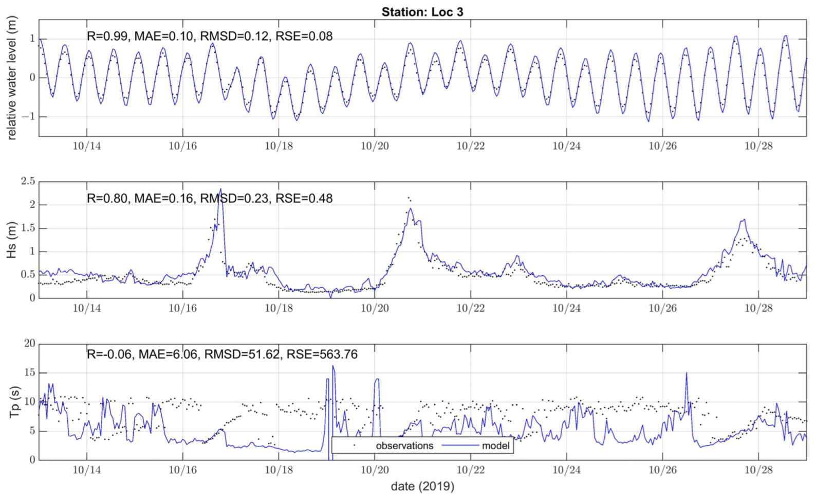
	Loc 3	0.99	0.10	0.12	0.08
Significant wave height	Loc 2	0.69	0.29	0.34	1.99
	Loc 3	0.80	0.16	0.23	0.48

using the following equations:

$$\mathrm{R}=\frac{\sum _{\mathrm{i}=1}^{\mathrm{N}}({\mathrm{M}}_{\mathrm{i}}-\stackrel{-}{\mathrm{M}})({\mathrm{O}}_{\mathrm{i}}-\stackrel{-}{\mathrm{O}})}{\sqrt{\sum _{\mathrm{i}=1}^{\mathrm{N}}{({\mathrm{M}}_{\mathrm{i}}-\stackrel{-}{\mathrm{M}})}^2}\sqrt{\sum _{\mathrm{i}=1}^{\mathrm{N}}{({\mathrm{O}}_{\mathrm{i}}-\stackrel{-}{\mathrm{O}})}^2}}$$

(6)

$$\mathrm{M}\mathrm{A}\mathrm{E}=\frac{1}{\mathrm{N}}\sum _{\mathrm{i}=1}^{\mathrm{N}}\left|{\mathrm{M}}_{\mathrm{i}}-{\mathrm{O}}_{\mathrm{i}}\right|$$

(7)

$$\mathrm{R}\mathrm{M}\mathrm{S}\mathrm{D}=\sqrt{\frac{1}{\mathrm{N}}\sum _{\mathrm{i}=1}^{\mathrm{N}}{\left({\mathrm{O}}_{\mathrm{i}}-{\mathrm{M}}_{\mathrm{i}}\right)}^2}$$

(8)

$$\mathrm{R}\mathrm{S}\mathrm{E}=\frac{{\sum }_{\mathrm{i}=1}^{\mathrm{N}}{\left({\mathrm{O}}_{\mathrm{i}}-{\mathrm{M}}_{\mathrm{i}}\right)}^2}{{\sum }_{\mathrm{i}=1}^{\mathrm{N}}{(\stackrel{-}{\mathrm{O}}-{\mathrm{O}}_{\mathrm{i}})}^2}$$

(9)

where M is the model output, O is the observed data, and N is the total number of data points.

Smaller values of MAE, RMSD and RSE indicate a better fit between the model output and the measured data, whereas larger values suggest the opposite. The Pearson product-moment correlation coefficient, R, measures the phasing between the model output and observed data [59] and consequently, determines how well the water surface elevation (or wave height) peaks and troughs line up. The value of R ranges from −1.0 to +1.0, where a value equal or close to +1.0 is preferred. A value equal to or close to +1 means that the peaks and troughs of model output match the observed data. Table 1 shows that the wave height and relative water level R values are above 0.8 for all stations except for wave height at Loc 2. The MAE and RMSD values were less than 0.25 m for all the locations except at Loc 2 which shows MAE of 0.29 m and RMSD of 0.34 m for wave height (Table 1). The RSE indicates the significance of the difference between the model output and observed data at each location. Water surface elevation RSE values were low (i.e., less than 0.25) for all the locations. Larger RSE values were found for wave height at locations near CI and close to the ebb tidal delta (Loc 2, Loc 3—Figure 4 and Figure 5). The larger variance at these locations is likely due to the influence of the bottom roughness and the shape and form of the sand shoals and nearshore bathymetry, on incoming waves.

Sediment Transport and Morphology

For this study, the sediment-transport model was calibrated by comparing predictions of sediment fluxes alongshore to observations or estimates of alongshore transport from previous studies. Model predictions were compared to historical estimates of longshore sediment-transport rates along the southern portion of Assateague Island at a series of cross-sections implemented in the model domain at locations where historical estimates of longshore sediment transport existed [29,60]. Each cross section started near the shoreline at the dune crest and extended to the 7 m isobath representing the upper to middle shoreface and varied in length from 2.5 to 3.25 km (Figure 1). According to Finkelstein [60], the average net longshore transport along southern Assateague Island was 165,000 m³ per year during the period 1859 to 1983. The model presented here predicted the net longshore sediment transport along the southern Assateague Island to be approximately 36,000 m³ (transect location AS_N5 in Figure 1B) for a two-month period (September—October, 2019) which included low-energy conditions (i.e., tidal) and high-energy events (i.e., three nor-easters and one tropical storm, Hurricane Dorian). Previous studies [61] reported that an average of 18 storms per year made landfall across the northeastern coast of the United States between 2000 and 2019. To make the predicted transport rates during the simulation period comparable to previous estimates [60], and to match the number of storms within the simulation period to those reported in the literature [60,61], the model-predicted transport was multiplied by a factor of 4.5. The resulting net longshore transport was 162,000 m³, which is comparable to previously reported rates of approximately 165,000 m³/yr [24,60]. This is reasonable result considering sediment-transport predictions are generally acceptable if they differ with observations by a factor of two [62]. In addition, the model was compared with bathymetric surveys collected in the vicinity of CI [27] to determine if the order of change in the morphology predicted by the model was of the same order as those measured in the field between 2019 and 2020. The difference in bathymetry between the surveys shows that morphology changes vary between 0.1 and 1.5 m along the broad flood-tidal delta platform and inlet throat, 0.1 to 1.0 m along the ETD area and of the order of 1–2 m at the inlet. Model predictions show changes of the same order, ranging from 0.1 to 1.0 m throughout the flood-tidal delta and CI throat, 0.1–0.6 m along the ETD, and between 0.1 and 1.5 m at CI (see Figure S6).

3. Results

3.1. Tidal and Subtidal Water and Sediment Exchange

The Chincoteague Island backbarrier basin exchanges tidal flows through CI and Ocean City Inlet (Figure 1). Three cross sections (CS1, CS2, and CS3) were considered to analyze the simulated tidal flow exchange (Figure 1B). Most of the tidal inflow enters the backbarrier bay through CI seaward of Chincoteague Island (CS1 in Figure 1C). The remaining flow enters through Ocean City Inlet and is directed south toward the backbarrier basin (OCS in Figure 1C). Flow through CI (CS1 in Figure 1C) ranges between 4000 and 6000 m³/s during neap and spring conditions, respectively, and can reach or exceed 8000 m³/s during storms (Figure 6A). For the Chincoteague channel near the town of Chincoteague (CS3 in Figure 1B), flows range from 1000–1600 m³/s during neap tides to 3000 m³/s during spring tides, with flows exceeding 3000 m³/s during storms (Figure 6C). At the inlet leading to the Wallops backbarrier basin (CS2 in Figure 1B), flows range from 600–700 m³/s during neap tides, to 1300 m³/s during spring tides, and up to 1800 m³/s during storms (Figure 6B). Ocean City Inlet southerly flows range from 300–500 m³/s during neap tides to 600–700 m³/s during spring tide conditions and reach or exceed 1000 m³/s during storms (Figure 6D).

The cumulative volume of water exchanged at these inlets resulting from the two-month simulation (i.e., tidal prism) is 6.76 × 10⁷ m³ for the main CI (CS1; Figure 1B), 3.48 × 10⁷ m³ at the Chincoteague Island main channel near the Town (CS3; Figure 1B), 1.86 × 10⁷ m³ for the backbarrier of Wallops Island, and 1.0 × 10⁷ m³ for Ocean City Inlet south (OCS in Figure 1C). The simulation period did include Hurricane Dorian (6–9 September 2019) and three nor’easters in October of 2019, all events of which could mildly influence the calculated tidal prism.

Tidal and subtidal exchange and corresponding sediment transport at the inlets vary proportionally from neap to spring tide conditions and exhibit higher sediment-transport magnitudes during storms. The transport magnitude is a function of the combined influence of surge elevation, waves heights, and the tidal flow magnitude exchanged through the inlets (Figure 7A–F). For the simulation period (9/1 through 10/30, 2019), the corresponding maximum tidal height reached 1.2 m during spring maximum before the peak of Hurricane Dorian, with wave heights approaching 0.75 m (~9/2–9/3; Figure 7G). Storm surge heights increased by 30 cm, reaching 1.5 m, and wave heights doubled nearing 1.5 m, respectively, during the storm’s peak (~9/7; Figure 7G). As a result, the subtidal water level rose nearly 0.7 m during Dorian (~9/7; Figure 7G) and subsided to normal levels three days after the storm (~9/10). During the period where nor’easters were evaluated later in October of the same year, tidal heights were similar to those in September; however, wave heights were lower in magnitude, ranging from 0.2 to 0.3 m ahead of each storm (Figure 7H). As a result, subtidal water levels typically rose 0.25 m for two weaker nor’easters documented (10/16, 10/28; Figure 7H) and up to 0.45 m for a stronger nor’easter reported on 10/21 (Figure 7H). Wave heights before the storms were approximately 0.3–0.4 m and ranged from 1.7 to 2.3 m at the storm peak.

Sediment-transport magnitude varied at each inlet proportionally to the hydrodynamic conditions. During spring tidal conditions ahead of Hurricane Dorian, total instantaneous sediment flux at the main CI cross section (CS1) peaked at approximately 0.09–0.1 m³/s during flood (mid 9/2) and 0.2–0.22 m³/s during peak ebb (9/2–9/3), with peaks reaching 0.15 m³/s during the flooding surge of Hurricane Dorian, and approximately 0.25 m³/s during the ebbing surge (9/6–9/7) when the backbarrier was draining post landfall (Figure 7A). Mud transport dominates the total sediment-transport volumes at this inlet (CS1) which peaks during spring tides. It declines proportionally to the tidal range decline toward neap tide conditions, and exhibits a small tidal asymmetry (Figure 7A). Sand flux is a fraction of the total transport and ranges from 30 to 60%. Sand flux is strongly ebb-dominant during spring tides (0.05 m³/s during flood; and 0.12 m³/s during ebb), weakly ebb dominant during neap tides (0.03 m³/s during flood; and 0.06 m³/s during ebb), strongly flood dominant during Hurricane Dorian (0.08 m³/s during flood; and 0.13 m³/s during ebb; Figure 7A). Sediment flux trends were similar but proportionally lower in magnitude for CS2 and CS3. Model results suggest that sand flux at these inlets (CS2; CS3) was generally lower in magnitude and showed less asymmetric trends compared to CS1. However, during nor’easters, as expected, sand flux can increase appreciably (Figure 7D,F). Sand exhibits ample mobility during peak ebb conditions at the highest tidal range (~10/15) and is ebb dominant, switching to flood dominant during all nor’easters. Sand flux is also proportional to the magnitude of the event; for instance, the first nor’easter (~10/17) reversed seaward sand flux from 0.02 m³/s to landward flux of similar order. Following the nor’easter, the sand transport diminished to negligible transport during neap conditions (on 10/20) prior to the next event. At the onset of the second, and stronger nor’easter, sand flux initially peaked in the seaward direction (0.03 m³/s) and the storm gradually reversed the transport direction to weekly flood dominant and subsequently returned to background tidal flux for several days after the storm passed. Contrastingly, at the onset of the third storm of the month of October 2019, sand flux gradually peaked from neap to spring conditions (from 10/23 to 10/27) leading to the storm (~10/28) reaching magnitudes of 0.05 m³/s (ebb) ahead of the storm; however, sand flux as the storm was passing became and remained weekly flood dominant (0.01 m³/s) or at net zero, offsetting the next ebb peak from the falling tide, before gradually returning to normal (pre-storm tidal) magnitudes of transport by October 29. This suggests that changes in storm characteristics among the winter storms contribute to differences in the timing and magnitude of surge heights and waves, which result in changes in sediment transport influencing sediment budgets in the study area (Figure 7 and

Table 2. Ranges of instantaneous volumetric sediment fluxes for all sediment classes during background tidal and during storm conditions.

Cross-Section Location	Background Tidal (m3/s)		Hurricane Dorian (m3/s)		Nor’easters (m3/s)
	Flood	Ebb	Flood Surge	Ebb Surge	Flood Surge	Ebb Surge
CS1	0.8–0.11	0.04–0.07	0.17	0.27	0.22–0.34	0.34–0.70
CS2	0.02–0.04	0.02–0.04	0.13	0.08	0.05–0.15	0.15–0.26
CS3	0.025–0.06	0.05–0.075	0.17	0.15	0.07–0.21	0.10–0.15

).

3.2. Coastal Sediment Budgets

Model results for the simulation period suggest a southern movement of sediment along southern Assateague Island (cross sections AS_N3, AS_N4, AS_N5 in Figure 8A; see Figure 1B for locations), and show that a large percentage of the southward-directed longshore transport is conveyed around Fishing Point (cross sections FE_N in Figure 8A; see Figure 1B for locations). Cumulative sediment volumes (all sediment classes) are uniform along the southern Assateague Island and range from 44,473 to 54,025 m³ for September and October of 2019 (Figure 8A), suggesting a spatially uniform transport rate for the entire simulation period. Similarly, transport volumes for sand of all simulated classes (very fine, fine, and medium sand) were similar along the southern Assateague Island cross section and varied in the range 3748–8426 m³ (medium sand), 1552–12,282 m³ (fine sand), and 27,287–35,401 m³ (very fine sand), respectively (Figure 8A). The sharp reduction at the next transect location along Fishing Point (cross section FW_N in Figure 8A) suggests that most of the southward-transported sediment is either deposited along the beach before it reaches this location (FW_N), or it is lost to a deeper water sink south of the point). The transport volumes downdrift of CI decline sharply, to less than 10,000 m³; albeit similar fractions of sand and mud (Figure 8A) are transported downdrift towards CI (CS1).

It is tempting to assume that most of the sediment from the southernmost location on the ocean-facing shoreline of Assateague Island (AS_N5 in Figure 1B) is transported along Fishing Point toward the eastern cross section (FE_N) because the sediment volumes are of the same order. However, the declines in sediment volume at this downdrift location (FW_N) imply differently. Rather, the results suggest the following (Figure 8A): that (1) either the sediment is deposited between the easternmost (FE_N) and westernmost (FW_N) transects locations along Fishing Point, or (2) that the sediment directed southward from Assateague Island is deposited to a deeper water sink east of the Fishing Point (FE_N), and subsequently re-entrained and transported to the west and is deposited between the east (FE_N) and west (FW_N) locations. The model results suggest that the sediment transported from southern Assateague Island around the spit are not originating from the same transport processes, and further, that the shape of the spit in its current configuration hinders sediment delivery to the inlet (Figure 8). The likely deposition of sediment along the terminus of the Fishing Point spit is also evidenced as a decline in the size of the transport vectors for sand (Figure 9A) and total sediment (Figure 9B) near the terminus, corroborating the volumetric sediment budgets (Figure 8A).

Along the Wallops Island shoreline (Figure 8C) transport gradually increases from the north (transect WN_N1; shown in Figure 1C) toward the south approaching Wachapreague Inlet (transect WS_N7; shown in Figure 1C). While the model does not show the presence of a nodal zone for mud, it does show one for sand (near transects WN_N1 and WS_N2). North of this location, coarser sand (medium sand and fine sand) is transported northward, while south of this location both sand and mud is transported southward, with an increasing rate. Total transport gradually increases from 5939 m³ (WN_N2, north) to approximately 52,713 m³ (WS_N7, south; Figure 8C). At this southernmost location volumetric transport reaches a similar order of sediment transport to that predicted at southern Assateague (Figure 8A). Sand transport for all sand classes (medium, fine, and very fine) shows similar trends as total transport, with very fine sand increasing from 2143 m³ (north) to nearly 9105 m³ (south), while medium and fine sand combined reach 5050 m³ north of the nodal point (WN_N2) and 59,961 m³ toward the south, south of the nodal point (WS_N7).

Transport trends predicted by the model agree with general trends previously reported by other studies based on annualized estimates [24,63,64,65]), regional sand trapping estimates [23], and recent analysis of sediment loss/gain rates along the entire Eastern Shore barrier-island chain [66]. In particular, the model shows that Fishing Point traps approximately 70–90% of the sediment transported along southern Assateague Island (Figure 8A), which is of the same order as the sand budgets recently reported [66], where the sand change volume within Fishing Point (29 ± 1.3 × 10⁴) is approximately 73% of the sand volume change of southern Assateague (38 ± 1.7 × 10⁴). Similarly, the model predicts sand transport volumes decline sharply, following sand trapping along Fishing Point, revealing that sediment-transport rates at Wallops Island are at least 20% lower toward the north, and gradually increase to the south (Figure 8C). The predicted rates are similar to previous studies [23,67], and in agreement with predictions of parallel retreat behavior for Wallops Island and other Islands to the south. Moreover, the trapped sand because of the elongation of southern Assateague Island and the rapid growth of Fishing Point starves the downdrift barrier of sand [23,66,68]. The predicted overall trends by the model, coupled with the overall validation of modern transport rates with recent observations and sand transport estimates allow for the model to be used to investigate in more detail and at local scales what drives the regional behaviors previously observed, and help elucidate specific processes in a spatially explicit manner.

3.3. Spatial Patterns of Sediment Transport

Residual sediment-transport patterns for the conditions evaluated using the model, which included Hurricane Dorian, and three nor’easters, show spatially explicit patterns for the various sediment classes and reveal associated governing processes (Figure 9). Along southern Assateague, coarser sand (fine and medium; Figure 9A) moves onshore (blue and green vectors; Figure 9A), while very fine sand (red vectors) is directed to the south–southwest along the shoreline. Upon reaching Fishing Point, sand traveling near the beach is directed around Fishing Point toward the spit terminus, while sand moving some distance away from the coastline continues to the southwest, bypassing the Point. Offshore of Assateague Island, sand is also mobile along the shoreface, activating sand ridges to the southeast of the Fishing Point. Within the inlet throat of the lower channel, sand is moving offshore, indicating that the channel is ebb-dominant during the conditions evaluated (Figure 9A). Along the distal ETD, mud and very fine sand (black and red vectors; Figure 9B,D) are directed seaward (south to southwest heading), indicating export, while coarser sand is directed west-northwest (Figure 9C). The offshore magnitude of transport for very fine sand and mud is twice that of fine and medium sand to the west-northwest (Figure 9B). The western margin of the ETD near the channel margins experiences similar residual sediment-transport trends as the distal ETD, except that both very fine and fine sand move seaward to the south, with lower magnitudes of medium sand directed to the southwest at sufficiently shallow water depths (Figure 9A,C). The shallow section of the western margin of the ETD shows significant re-working of sand across all sediment classes (Figure 9A,C). Model results show that sand (medium and fine) is transported to the northwest towards the northern end of Wallops Island at higher rates compared to the sand that is transported west along the distal ETD and proximal main channel, and—contrary to processes along the distal ETD—very fine sand is also transported in the same direction as the coarser sand fractions (Figure 9A,C).

4. Summary and Discussion

The elongation of Fishing Point over the last 100 years produced significant changes in the morphology of downdrift coastal compartments [66,68,69] by starving downdrift barriers of sand and has long been attributed to the rapid migration of the four barrier islands south of Assateague [69]. Other studies showed that the growth of Fishing Point sequesters most of the sand reaching southern Assateague Island through longshore transport [23], and that the spit elongation influenced longshore transport trends along Wallops Island [63]. For instance, southern Assateague Island’s elongation and southern progradation, beyond trapping sand, likely influenced longshore sand delivery to downdrift barriers and altered transport gradients [66]. In addition, the elongation gradually shelters the waves approaching at an angle to the coast from the northeast quadrant, which influences alongshore sediment flux to the south [70]. It has the potential to both change the nodal zone of alongshore sediment-transport divergence as well as migrate or create new erosional hotspots [63,64,66].

Our modeling set-up, calibration, and simulations allowed for quantitative analysis of hydrodynamics and sediment-transport trends that included the following: (1) water exchange volumes and corresponding tidal prism evaluation between the ocean and the backbarrier of Chincoteague and Assateague islands during background non-storm, as well as storm conditions, (2) volumetric sediment exchange among all sediment classes for all inlets contributing to the tidal prism of Chincoteague Bay, (3) the calculation of coastal sediment budgets via analysis of detailed alongshore sediment-transport rates by sediment class, and finally (4) detailed spatial patterns of residual transport for all sediment classes.

The conditions evaluated with the simulations in this study included mixed environmental drivers, such as background tidal forcings and the inclusion of a tropical storm (e.g., Hurricane Dorian) and three extra tropical storms (nor-easters). Model results suggest that a portion of the sand that is transported south along the southern Assateague Island continues to the south, bypassing Fishing Point, while some continues around the spit toward the spit terminus, inlet and flood and ETD. The model also showed that transport rates diminish rapidly shortly beyond the terminus of the spit, a result that corroborates analysis presented by previous research [23,66,68], which reported in a more qualitative manner that Fishing Point spit elongation starved downdrift barriers. More recent analysis also demonstrated that the spit elongation reduced the volume of sediment delivered to the updrift margin of CI, contributed to the expansion of CI, and reduced sediment bypassing [71].

Model results suggest that the residual sediment-transport pathways vary among the different grain sizes (Figure 9), as reported and corroborated by studies of similar barrier-inlet systems in the East Frisian Islands, Germany [4,18]. Moreover, the spatial patterns of residual sediment transport reveal distinctive pathways for sand movement in this system, elucidating the surface processes that govern sand transport here, and in other mixed-energy barrier-island systems elsewhere. Finally, leveraging model results permits the development of coastal sediment budgets, enhancing our understanding of sand transport, and informing regional sand-resource and shoreline management.

References

- Davis, R.A.; FitzGerald, D.M. Beaches and Coasts, 2nd ed.; John Wiley & Sons: Hoboken, NJ, USA, 2020; ISBN 978-1-119-33451-4. [Google Scholar]
- McBride, R.A.; Anderson, J.B.; Buynevich, I.V.; Byrnes, M.R.; Cleary, W.; Fenster, M.S.; FitzGerald, D.M.; Hapke, C.J.; Harris, M.S.; Hein, C.J.; et al. Morphodynamics of Modern and Ancient Barrier Systems: An Updated and Expanded Synthesis. Earth Syst. Environ. Sci. 2022, 10, 289–417. [Google Scholar] [CrossRef]
- Hayes, M. Barrier Island Morphology as a Function of Tidal and Wave Regime. In Barrier Islands: From the Gulf of St. Lawrence to the Gulf of Mexico; Academic Press: London, UK, 1979; pp. 1–27. [Google Scholar]
- Herrling, G.; Winter, C. Tidal Inlet Sediment Bypassing at Mixed-Energy Barrier Islands. Coast. Eng. 2018, 140, 342–354. [Google Scholar] [CrossRef]
- FitzGerald, D.M. Shoreline Erosional-Depositional Processes Associated with Tidal Inlets. Lect. Notes Coast. Estuar. Stud. 1988, 29, 186–225. [Google Scholar]
- de Swart, H.E.; Zimmerman, J.T.F. Morphodynamics of Tidal Inlet Systems. Annu. Rev. Fluid Mech. 2009, 41, 203–229. [Google Scholar] [CrossRef]
- Fenster, M.; Dolan, R. Assessing the Impact of Tidal Inlets on Adjacent Barrier Island Shorelines. J. Coast. Res. 1996, 12, 294–310. [Google Scholar]
- FitzGerald, D.M.; Buynevich, I.; Hein, C. Morphodynamics and Facies Architecture of Tidal Inlets and Tidal Deltas. In Principles of Tidal Sedimentology; Springer Netherlands: Dordrecht, The Netherlands, 2010; pp. 301–333. ISBN 978-94-007-0123-6. [Google Scholar]
- Oertel, G.f. Processes of Sediment Exchange between Tidal Inlets, Ebb Deltas and Barrier Islands. In Hydrodynamics and Sediment Dynamics of Tidal Inlets; American Geophysical Union (AGU): Washington, DC, USA, 1988; pp. 297–318. ISBN 978-1-118-66924-2. [Google Scholar]
- Wang, Z.B.; Hoekstra, P.; Burchard, H.; Ridderinkhof, H.; De Swart, H.E.; Stive, M.J.F. Morphodynamics of the Wadden Sea and Its Barrier Island System. Ocean Coast. Manag. 2012, 68, 39–57. [Google Scholar] [CrossRef]
- Kraus, N.C.; Mark, D.J.; Sarruff, M.S. DMS: Diagnostic Modeling System. Report 1, Reduction of Sediment Shoaling by Relocation of the Gulf Intracoastal Waterway, Matagorda Bay, Texas. In This Digital Resource Was Created from Scans of the Print Resource; Coastal and Hydraulics Laboratory (U.S.) Engineer Research and Development Center (U.S.): Vicksburg, MS, USA, 2000. [Google Scholar]
- de Vriend, H.J.; Bakker, W.T.; Bilse, D.P. A Morphological Behaviour Model for the Outer Delta of Mixed-Energy Tidal Inlets. Coast. Eng. 1994, 23, 305–327. [Google Scholar] [CrossRef]
- Nienhuis, J.H.; Ashton, A.D. Mechanics and Rates of Tidal Inlet Migration: Modeling and Application to Natural Examples. J. Geophys. Res. Earth Surf. 2016, 121, 2118–2139. [Google Scholar] [CrossRef]
- Nienhuis, J.H.; Lorenzo-Trueba, J. Simulating Barrier Island Response to Sea Level Rise with the Barrier Island and Inlet Environment (BRIE) Model v1.0. Geosci. Model Dev. 2019, 12, 4013–4030. [Google Scholar] [CrossRef]
- Lesser, G.R.; Roelvink, J.A.; van Kester, J.A.T.M.; Stelling, G.S. Development and Validation of a Three-Dimensional Morphological Model. Coast. Eng. 2004, 51, 883–915. [Google Scholar] [CrossRef]
- Dodet, G.; Bertin, X.; Bruneau, N.; Fortunato, A.B.; Nahon, A.; Roland, A. Wave-Current Interactions in a Wave-Dominated Tidal Inlet. J. Geophys. Res. Ocean. 2013, 118, 1587–1605. [Google Scholar] [CrossRef]
- Elias, E.P.L.; Cleveringa, J.; Buijsman, M.C.; Roelvink, J.A.; Stive, M.J.F. Field and Model Data Analysis of Sand Transport Patterns in Texel Tidal Inlet (the Netherlands). Coast. Eng. 2006, 53, 505–529. [Google Scholar] [CrossRef]
- Herrling, G.; Winter, C. Morphological and Sedimentological Response of a Mixed-Energy Barrier Island Tidal Inlet to Storm and Fair-Weather Conditions. Earth Surf. Dynam. 2014, 2, 363–382. [Google Scholar] [CrossRef]
- Roelvink, J.A.; Dastgheib, A. Long-Term Process-Based Morphological Modeling of Large Tidal Basins; CRC Press/Balkema: Boca Raton, FL, USA, 2012. [Google Scholar]
- Nahon, A.; Bertin, X.; Fortunato, A.B.; Oliveira, A. Process-Based 2DH Morphodynamic Modeling of Tidal Inlets: A Comparison with Empirical Classifications and Theories. Mar. Geol. 2012, 291–294, 1–11. [Google Scholar] [CrossRef]
- Ridderinkhof, W.; de Swart, H.E.; van der Vegt, M.; Hoekstra, P. Modeling the Growth and Migration of Sandy Shoals on Ebb-Tidal Deltas. J. Geophys. Res. Earth Surf. 2016, 121, 1351–1372. [Google Scholar] [CrossRef]
- Tung, T.T.; Walstra, D.; de Graaff, J.V.; Stive, M.J.F. Morphological Modeling of Tidal Inlet Migration and Closure. Available online: https://www.jstor.org/stable/25737953 (accessed on 21 August 2022).
- Shawler, J.L.; Hein, C.J.; Obara, C.A.; Robbins, M.G.; Huot, S.; Fenster, M.S. The Effect of Coastal Landform Development on Decadal-to Millennial-Scale Longshore Sediment Fluxes: Evidence from the Holocene Evolution of the Central Mid-Atlantic Coast, USA. Quat. Sci. Rev. 2021, 267, 107096. [Google Scholar] [CrossRef]
- Fenster, M.S.; McBride, R.A. Barrier-Island Geology and Morphodynamics along the Open-Ocean Coast of the Delmarva Peninsula: An Overview. In Tripping from the Fall Line: Field Excursions for the GSA Annual Meeting, Baltimore; Geological Society of America: Boulder, CO, USA, 2015; Volume 40, pp. 310–334. [Google Scholar]
- Krantz, D.; Hobbs, C.; Wikel, G. Atlantic Coast and Inner Shelf. In The Geology of Virginia; William & Mary: Williamsburg, VA, USA, 2016. [Google Scholar]
- Sakib, M.M.; Georgiou, I.; Hein, C.; Fenster, M.; Zou, S.; Esposito, C.; Foster-Martinez, M.; Messina, F.; Trembanis, A. Mechanisms and Rates of Sand Bypassing along a Rapidly Evolving Inlet-Spit System. In Proceedings of the AGU Fall Meeting 2021, New Orleans, LA, USA, 13–17 December 2021. [Google Scholar]
- McPherran, K.A.; Dohner, S.M.; Trembanis, A.C. A Comparison of the Temporal Evolution of Hydrodynamics and Inlet Morphology during Tropical Storm Fay (2020). Shore Beach 2021, 89, 11–22. [Google Scholar] [CrossRef]
- Nowacki, D.J.; Ganju, N.K. Storm Impacts on Hydrodynamics and Suspended-Sediment Fluxes in a Microtidal Back-Barrier Estuary. Mar. Geol. 2018, 404, 1–14. [Google Scholar] [CrossRef]
- McBride, R.A.; Fenster, M.S.; Seminack, C.T.; Richardson, T.M.; Sepanik, J.M.; Hanley, J.T.; Bundick, J.A.; Tedder, E. Holocene Barrier-Island Geology and Morphodynamics of the Maryland and Virginia Open-Ocean Coasts: Fenwick, Assateague, Chincoteague, Wallops, Cedar, and Parramore Islands. In Tripping from the Fall Line: Field Excursions for the GSA Annual Meeting, Baltimore, 2015; Geological Society of America: Boulder, CO, USA, 2015. [Google Scholar] [CrossRef]
- Carruthers, T.; Beckert, K.; Dennison, B.; Thomas, J.; Saxby, T.; Williams, M. Assateague Island National Seashore Natural Resource Condition Assessment: Maryland, Virginia; Natural Resource Report NPS/ASIS/NRR—2011/405; National Park Service: Fort Collins, CO, USA, 2011. [Google Scholar]
- Kang, X.; Xia, M.; Pitula, J.S.; Chigbu, P. Dynamics of Water and Salt Exchange at Maryland Coastal Bays. Estuar. Coast. Shelf Sci. 2017, 189, 1–16. [Google Scholar] [CrossRef]
- Kang, X.; Xia, M. The Study of the Hurricane-Induced Storm Surge and Bay-Ocean Exchange Using a Nesting Model. Estuaries Coasts 2020, 43, 1610–1624. [Google Scholar] [CrossRef]
- Casey, J.; Wesche, A. Marine Benthic Survey of Maryland’s Coastal Bays: Part I, Spring and Summer Periods; Maryland Department of Natural Resources: Annapolis, MD, USA, 1981. [Google Scholar]
- Goodrich, D.M. On Meteorologically Induced Flushing in Three U.S. East Coast Estuaries. Estuar. Coast. Shelf Sci. 1988, 26, 111–121. [Google Scholar] [CrossRef]
- Cooperative Institute for Research in Environmental Sciences. Continuously Updated Digital Elevation Model (CUDEM)—1/9 Arc-Second Resolution Bathymetric-Topographic Tiles; Cooperative Institute for Research in Environmental Sciences: Boulder, CO, USA, 2014. [Google Scholar]
- Hiller, R.; Calder, B.; Hogarth, P.; Gee, L. Adapting CUBE for Phase Measuring Bathymetric Sonars; University of New Hampshire: Durham, NH, USA, 2005. [Google Scholar]
- Buczkowski, B.; Reid, J.A.; Schweitzer, P.N.; Cross, V.A.; Jenkins, C.J. UsSEABED: Offshore Surficial-Sediment Database for Samples Collected within the United States Exclusive Economic Zone; USGS: Reston, VA, USA, 2020. [Google Scholar] [CrossRef]
- Fenster, M.S.; Dolan, R.; Smith, J.J. Grain-Size Distributions and Coastal Morphodynamics along the Southern Maryland and Virginia Barrier Islands. Sedimentology 2016, 63, 809–823. [Google Scholar] [CrossRef]
- Folk, R.L. A Review of Grain-Size Parameters. Sedimentology 1966, 6, 73–93. [Google Scholar] [CrossRef]
- Deltares. Delft3D-FLOW: Simulation of Multidimensional Hydrodynamic Flows and Transport Phenomena, Including Sediments; Deltares: Delft, The Netherlands, 2014. [Google Scholar]
- Liu, K.; Chen, Q.; Hu, K.; Xu, K.; Twilley, R.R. Modeling Hurricane-Induced Wetland-Bay and Bay-Shelf Sediment Fluxes. Coast. Eng. 2018, 135, 77–90. [Google Scholar] [CrossRef]
- Sakib, M.; Nihal, F.; Haque, A.; Rahman, M.; Ali, M. Sundarban as a Buffer against Storm Surge Flooding. World J. Eng. Technol. 2015, 3, 59–64. [Google Scholar] [CrossRef]
- Salehi, M. Storm Surge and Wave Impact of Low-Probability Hurricanes on the Lower Delaware Bay—Calibration and Application. J. Mar. Sci. Eng. 2018, 6, 54. [Google Scholar] [CrossRef]
- Caldwell, R.L.; Edmonds, D.A. The Effects of Sediment Properties on Deltaic Processes and Morphologies: A Numerical Modeling Study. J. Geophys. Res. Earth Surf. 2014, 119, 961–982. [Google Scholar] [CrossRef]
- Hanegan, K.; Georgiou, I. Tidal Modulated Flow and Sediment Flux through Wax Lake Delta Distributary Channels: Implications for Delta Development. Proc. Int. Assoc. Hydrol. Sci. 2015, 367, 391–398. [Google Scholar] [CrossRef]
- Sakib, M.; Nihal, F.; Akter, R.; Maruf, M.; Akter, M.; Noor, S.; Rimi, R.A.; Haque, A.; Rahman, M. Afforestation as a Buffer against Storm Surge Flooding along the Bangladesh Coast. In Proceedings of the 12th International Conference on Hydroscience & Engineering, Tainan, Taiwan, 6–10 November 2016; p. 5. [Google Scholar]
- Sullivan, J.C.; Torres, R.; Garrett, A.; Blanton, J.; Alexander, C.; Robinson, M.; Moore, T.; Amft, J.; Hayes, D. Complexity in Salt Marsh Circulation for a Semienclosed Basin. J. Geophys. Res. Earth Surf. 2015, 120, 1973–1989. [Google Scholar] [CrossRef]
- Booij, N.; Ris, R.C.; Holthuijsen, L.H. A Third-Generation Wave Model for Coastal Regions 1. Model Description and Validation. J. Geophys. Res. Ocean. 1999, 104, 7649–7666. [Google Scholar] [CrossRef]
- Hajek, E.A.; Wolinsky, M.A. Simplified Process Modeling of River Avulsion and Alluvial Architecture: Connecting Models and Field Data. Sediment. Geol. 2012, 257–260, 1–30. [Google Scholar] [CrossRef]
- Leonardi, N.; Canestrelli, A.; Sun, T.; Fagherazzi, S. Effect of Tides on Mouth Bar Morphology and Hydrodynamics: Effect of Tides on Mouth Bar. J. Geophys. Res. Ocean. 2013, 118, 4169–4183. [Google Scholar] [CrossRef]
- Marciano, R.; Wang, Z.B.; Hibma, A.; de Vriend, H.J.; Defina, A. Modeling of Channel Patterns in Short Tidal Basins. J. Geophys. Res. Earth Surf. 2005, 110, F01001. [Google Scholar] [CrossRef]
- Nardin, W.; Mariotti, G.; Edmonds, D.A.; Guercio, R.; Fagherazzi, S. Growth of River Mouth Bars in Sheltered Bays in the Presence of Frontal Waves. J. Geophys. Res. Earth Surf. 2013, 118, 872–886. [Google Scholar] [CrossRef]
- van Rijn, L.C. Principles of Sediment Transport in Rivers, Estuaries and Coastal Seas; Aqua Publications: Amsterdam, The Netherlands, 1993. [Google Scholar]
- Partheniades, E. Erosion and Deposition of Cohesive Soils. J. Hydraul. Div. 1965, 91, 105–139. [Google Scholar] [CrossRef]
- Dietrich, J.C.; Westerink, J.J.; Kennedy, A.B.; Smith, J.M.; Jensen, R.E.; Zijlema, M.; Holthuijsen, L.H.; Dawson, C.; Luettich, R.A.; Powell, M.D.; et al. Hurricane Gustav (2008) Waves and Storm Surge: Hindcast, Synoptic Analysis, and Validation in Southern Louisiana. Mon. Weather Rev. 2011, 139, 2488–2522. [Google Scholar] [CrossRef]
- National Land Cover Database (NLCD), Ag Data Commons. Available online: https://data.nal.usda.gov/dataset/national-land-cover-database-2011-nlcd-2011 (accessed on 15 August 2022).
- Coon, W.F. Estimates of Roughness Coefficients for Selected Natural Stream Channels with Vegetated Banks in New York; U.S. Geological Survey; Earth Science Information Center, Open-File Reports Section [Distributor]; USGS: Ithaca, NY, USA, 1995. [Google Scholar]
- Nowacki, D.J.; Beudin, A.; Ganju, N.K. Spectral Wave Dissipation by Submerged Aquatic Vegetation in a Back-Barrier Estuary: Wave Dissipation by Vegetation. Limnol. Oceanogr. 2017, 62, 736–753. [Google Scholar] [CrossRef]
- Legates, D.R.; McCabe, G.J., Jr. Evaluating the Use of “Goodness-of-Fit” Measures in Hydrologic and Hydroclimatic Model Validation. Water Resour. Res. 1999, 35, 233–241. [Google Scholar] [CrossRef]
- Finkelstein, K. Cape Formation as a Cause of Erosion on Adjacent Shorelines. In Proceedings of the Coastal Zone’83; American Society of Civil Engineers: New York, NY, USA, 1983; pp. 620–640. [Google Scholar]
- Fritzen, R.; Lang, V.; Gensini, V.A. Trends and Variability of North American Cool-Season Extratropical Cyclones: 1979–2019. J. Appl. Meteorol. Climatol. 2021, 60, 1319–1331. [Google Scholar] [CrossRef]
- Wilcock, P.R. Toward a Practical Method for Estimating Sediment-Transport Rates in Gravel-Bed Rivers. Earth Surf. Process. Landf. 2001, 26, 1395–1408. [Google Scholar] [CrossRef]
- Fenster, M.S.; Bundick, J.A. Morphodynamics of Wallops Island, Virginia: A Mixed-Energy, Human-Modified Barrier Island. In Tripping from the Fall Line: Field Excursions for the GSA Annual Meeting, Baltimore, 2015: Geological Society of America Field Guide 40; Geological Society of America: Boulder, CO, USA, 2015; Volume 40, pp. 358–370. [Google Scholar]
- King, D.B., Jr.; Ward, D.L.; Hudgins, M.H.; Williams, G.G. Storm Damage Reduction Project Design for Wallops Island, Virginia. In Version 1.01: Engineer Research and Development Center, Vicksburg, MS, Coastal and Hydraulics Lab, Report No. ERDC/LAB TR-11-9; United States Army Corps of Engineers: Norfolk, VA, USA, 2010; p. 197. [Google Scholar]
- Moffatt, N. Wallops Island Shore Protection Study; NASA/Goddard Space Flight Facility: Wallops Island, VA, USA, 1986; p. 86. [Google Scholar]
- Robbins, M.G.; Shawler, J.L.; Hein, C.J. Contribution of Longshore Sand Exchanges to Mesoscale Barrier-Island Behavior: Insights from the Virginia Barrier Islands, U.S. East Coast. Geomorphology 2022, 403, 108163. [Google Scholar] [CrossRef]
- Headland, J.R.; Vallianos, L.; Shelden, J.G. Coastal Processes at Wallops Island, Virginia; American Society of Civil Engineers: New York, NY, USA, 1987; pp. 1305–1320. [Google Scholar]
- Hein, C.J.; Shawler, J.L.; De Camargo, J.M.; Klein, A.H.D.F.; Tenebruso, C.; Fenster, M.S. The Role Of Coastal Sediment Sinks in Modifying Longshore Sand Fluxes: Examples from the Coasts of Southern Brazil and the Mid-Atlantic USA. In Proceedings of the Coastal Sediments, Petersburg, FL, USA, 27–31 May 2019; World Scientific: Tampa/St. Petersburg, FL, USA, 2019; pp. 2330–2344. [Google Scholar]
- Rice, T.E.; Leatherman, S.P. Barrier Island Dynamics; the Eastern Shore of Virginia: Southeastern Geology. Southeast. Geol. 1983, 24, 125–137. [Google Scholar]
- Murray, B.; Ashton, A.D.; Coco, G. From Cusps to Capes: Self-Organised Shoreline Shapes. In Sandy Beach Morphodynamics; Elsevier: Amsterdam, The Netherlands, 2020; pp. 277–295. ISBN 978-0-08-102927-5. [Google Scholar]
- Sakib, M.M.; Messina, F.; Zou, S.; Bregman, M.; Georgiou, I.Y.; Hein, C.J.; Fenster, M.S. Spit Elongation And Re-Orientation Controls Downdrift Sediment Fluxes And Inlet Morphology; World Scientific: Singapore, 2023; pp. 90–102. [Google Scholar]