Article

Adaptive Graph-Learning Convolutional Network for Multi-Node Offshore Wind Speed Forecasting

1
College of Information Science & Technology, Zhejiang Shuren University, Hangzhou 310015, China
2
School of Computer Engineering and Science, Shanghai University, Shanghai 200444, China
*
Author to whom correspondence should be addressed.
J. Mar. Sci. Eng. 2023, 11(4), 879; https://doi.org/10.3390/jmse11040879
Submission received: 20 March 2023 / Revised: 16 April 2023 / Accepted: 19 April 2023 / Published: 21 April 2023
(This article belongs to the Special Issue Innovative Development of Offshore Wind Technology)

Abstract

:
Multi-node wind speed forecasting is greatly important for offshore wind power. It is a challenging task due to unknown complex spatial dependencies. Recently, graph neural networks (GNN) have been applied to wind forecasting because of their capability in modeling dependencies. However, existing methods usually require a pre-defined graph structure, which is not optimal for the downstream task and limits the application scope of GNN. In this paper, we propose adaptive graph-learning convolutional networks (AGLCN) that can automatically infer hidden associations among multi-nodes through a graph-learning module. It simultaneously integrates the temporal and graph convolutional modules to capture temporal and spatial features in the data. Experiments are conducted on real-world multi-node wind speed data from the China Sea. The results show that our model achieves state-of-the-art results in all multi-scale wind speed predictions. Moreover, the learned graph can reveal spatial correlations from a data-driven perspective.

1. Introduction

With the increase in energy consumption, the non-renewability of traditional energy sources and the emission of greenhouse gases, among other reasons, more and more countries are turning to renewable energy sources in industry [1,2,3]. Wind energy is basically a transformation of solar energy, with large energy reserves and no pollution, making it one of the best alternatives to fossil energy [4,5]. Therefore, mankind is actively researching the application prospects of wind power, and now, offshore wind power has become an important engine for green and sustainable development worldwide [6,7]. To ensure an uninterrupted power supply in the grid, it is imperative to continuously monitor and balance power generation and consumption, so an accurate and effective assessment of offshore wind power is essential [8]. It has been observed in the literature that wind power forecasting is typically based on wind speed forecasts [9,10]. Therefore, in order to protect the grid from uncertainty, power system managers and wind power companies need accurate forecasts of future wind speed [11]. On the time scale, wind speed forecasts can be divided into very-short-term forecasts, short-term forecasts, medium-term forecasts and long-term forecasts [12], where short-term wind speed forecasts are important for improving wind turbine generation efficiency and economic load dispatch planning, while medium- and long-term forecasts are mainly used for wind farm planning and generation planning to control and reduce operating costs [13,14]. In addition, the accurate prediction of wind speed is of great importance for climate analysis [15], biodiversity [16,17] and so on, so accurate prediction of offshore wind is of great importance [18].
Offshore wind prediction is a challenging task due to the high volatility, uncertainty and intermittency of offshore wind speed [19]. Wind speed prediction methods can fall into three main categories: physical, statistical machine-learning methods and deep learning methods [10,20,21]. The physical approaches [22] are to build systems (numerical weather prediction systems (NWP)). They use physical and meteorological variables to build a system based on thermodynamics and fluid mechanics, which has high calculation costs and is better suited to medium- and long-term planning [23]. The classical statistical methods, auto-regression integrated moving average (ARIMA) [19], assume the linear relationships of data. The machine learning methods, such as support vector regression (SVR) [24] and k-nearest neighbors (KNN) methods [25] show good performance in very-short-term and short-term wind forecasting. However, the statistical method ARIMA is incapable of capturing data’s nonlinear relationships and the machine learning methods actually simplify wind power prediction, which are unable to extract deep time series of feature information from complex wind speed data [26]. To address the limitations of the above methods, many scholars have begun to use a recurrent neural network (RNN) [27] and long short-term memory (LSTM) network [28] to perform the prediction tasks of wind speed with good results [29,30].
The above methods lead to inferior performance in multi-node wind speed prediction because they overlook spatial dependencies, so it is critical to capture the unknown spatial dependencies among multi-nodes. Z. Qiaomu et al. [31] proposed a predictive deep convolutional neural network (PDCNN), which exploits convolutional neural networks (CNN) to capture the spatial dependencies in wind data, to predict the wind speed of multiple stations at the same time. However, this method does not model the pair-wise dependencies among variables explicitly and cannot make full use of the spatial features of wind farms, which weakens the prediction performance [7]. Recently, graph neural networks (GNN) achieved great success in modeling relational dependencies of data due to their permutation invariance and local connectivity [32,33]. M. Yu et al. [7] connected all wind turbines in a certain range of wind farms by their geographical locations to form a graph to extract the spatial features of wind data for prediction. X. Geng et al. [
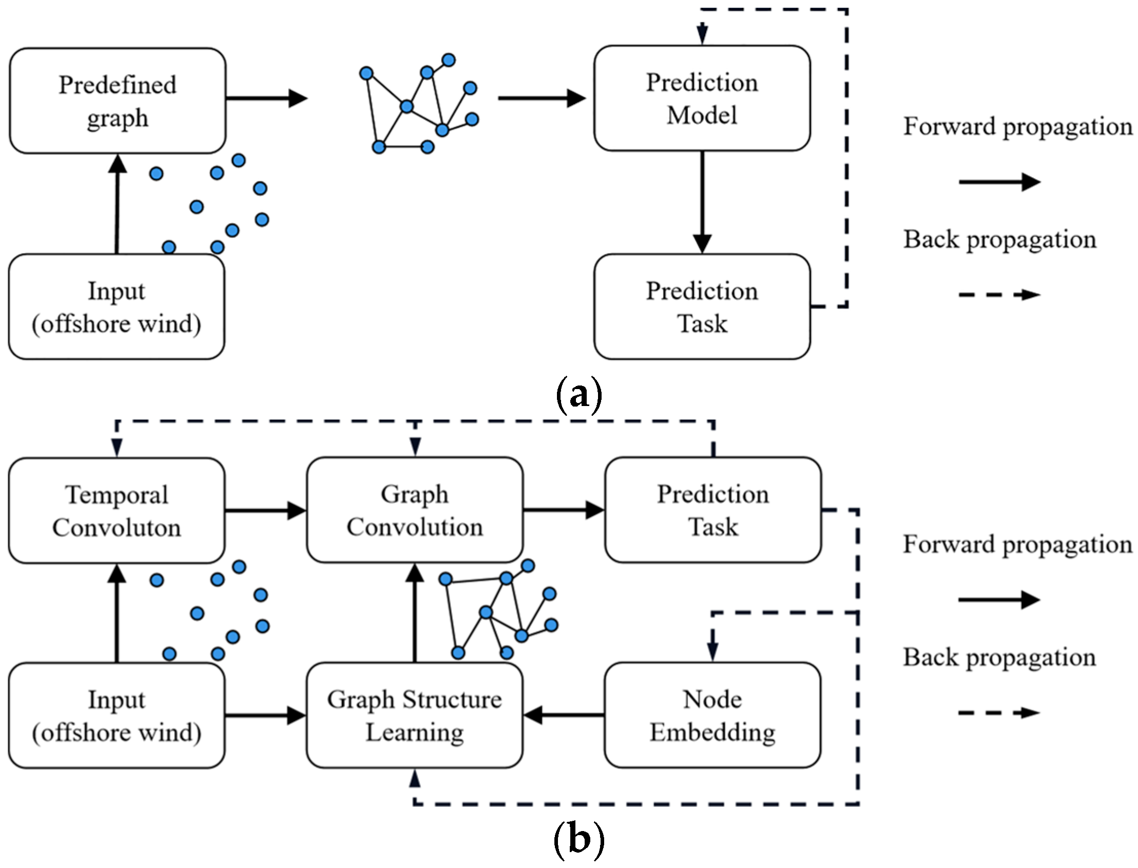
20] leveraged the geographic distance information of offshore wind nodes to construct a graph to predict multi-node offshore wind speed at the same time. These methods construct a predefined graph structure, as shown in Figure 1a.
Though remarkable success has been achieved by generalizing GNN to the wind speed forecasting domain, there are still several important problems that remain to be addressed: (1) Unknown spatial dependencies. Existing GNN approaches [7,20] applied to wind speed prediction rely heavily on a pre-defined graph structure in order to perform the forecasting task. These methods construct the graph structure based on assumed geographic location information. This method assumes that the spatial associations are equal to the geographic distance of multi-nodes, which is not flexible and representative enough to describe the correlations. The graph structure remains constant during the training of the network and is independent of the downstream tasks, which is not optimal for the multi-scale wind speed prediction task. (2) Graph structure learning and GNN learning. The current GNN approaches ignore the fact that graph structures are not optimal and need to be learned during training. How best to learn both graph structures of unknown associations and GNNs in an end-to-end framework is a challenging task.
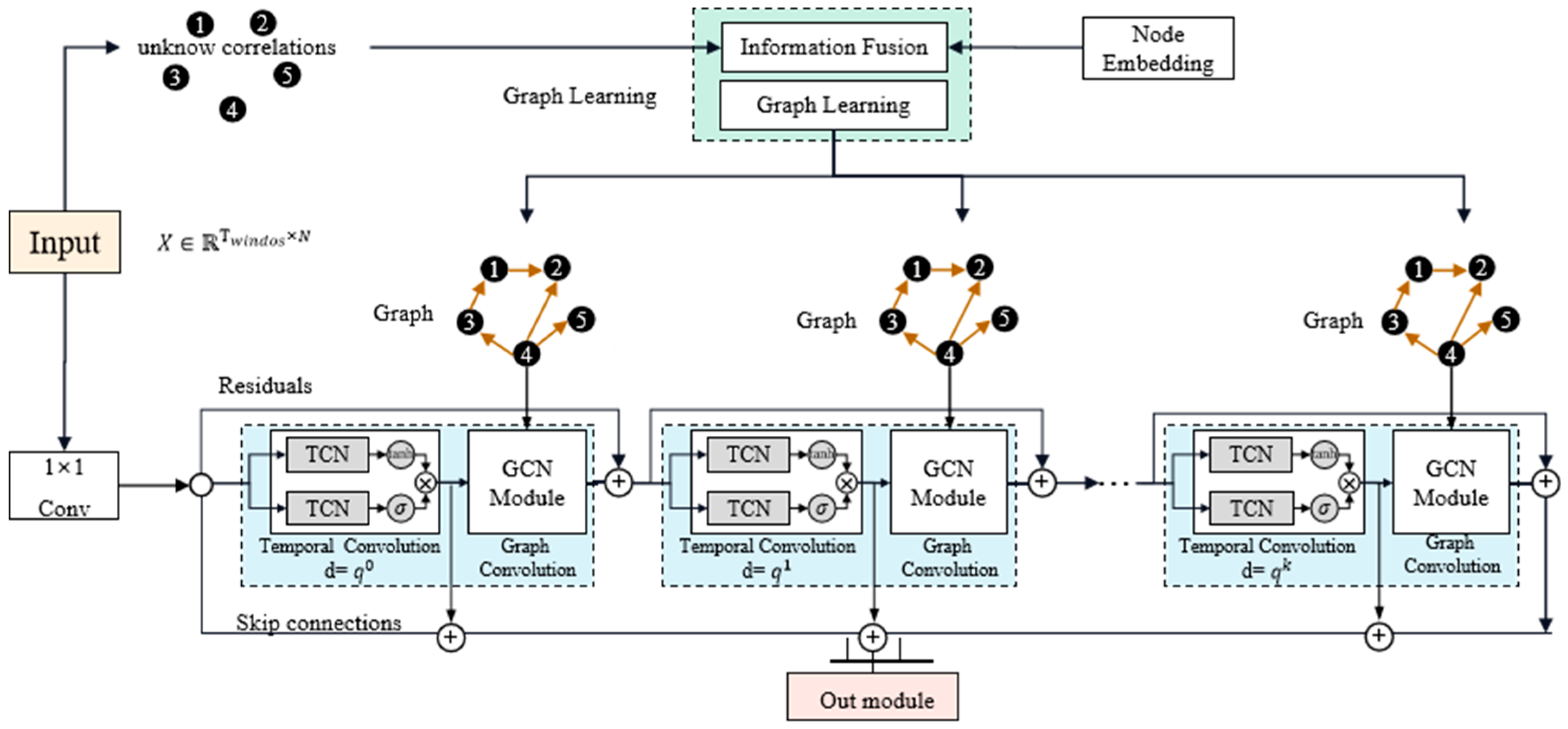
To cope with the above challenges, we propose an adaptive graph-learning convolutional network (AGLCN). Specifically, for challenge 1, an adaptive graph-learning method is proposed, which frees the need of GNN for a predefined structure. As shown in Figure 1, the graph structures are automatically inferred based on both dynamic wind speed data and trainable node embedding [34]. For challenge 2, the proposed network is an end-to-end framework, i.e., the parameters of the model can be learned via the gradient descent method. As shown in Figure 1b, the model on the highest level consists of three core components: graph learning, graph convolution and temporal convolution. Temporal convolution is used to extract the temporal relationship of data. Moreover, to avoid the gradient disappearance problems of RNN-based methods [35], we employ the CNN-based method because of its stable gradients and low memory requirements [36,37]. Graph convolution is used to capture the spatial feature of data based on the learned graph structure. Finally, the entire network is optimized based on predictive tasks. In summary, our main contributions are as follows:
  • We propose a novel graph-learning method to learn hidden associations in data, which does not require any prior knowledge as a guideline. It is more general than the existing GNN for wind speed prediction because our method can handle arbitrary multi-node time series without the need to pre-define the graph structure.
  • We design an end-to-end framework that integrates a graph structure learning module with temporal and graph convolution to achieve joint optimization, where temporal and graph convolution can efficiently extract temporal and spatial features.
  • Experiments on realistic multi-node wind speed forecasts show that our approach achieves optimal results for all comparative forecast scales (short-, medium- and long-term forecasts). Moreover, the graph structure learned by the model can be used to explore the correlation between multi-node wind speed from a data-driven perspective.
The rest of the paper is structured as follows: Section 2 presents the problem formulation and concept of GNN. The details of our framework are presented in Section 3. In Section 4, our experimental results show the effectiveness and efficiency of the proposed method. Section 5 presents the discussion. Section 6 offers conclusions of the paper.

2. Preliminary

Problem formulation. The target of multi-node offshore wind speed forecasting is to predict future multi-node values by exploiting historical data. Let x t R N denote the wind speed value monitored by N sensors at time step t, where x t [ i ] R denote the value of the ith sensor at time step t. Given a sequence of historical H time steps of observations on N sensors, X = { x t 1 , x t 2 , , x t h } R N × h , and our goal is to predict the values of future L-step for the N sensors, Y = { x t h + 1 , x t h + 2 , , x t h + L } R N × l . We aim to build a map f ( · ) from X to Y,
Y = f ( X )
A graph describes the relationships between nodes in a network. Thus, in the following, we provide a formal definition of graph-related concepts.
Definition 1.
(Graph). A graph is formulated as G = ( V , E ) where V R N represents the set of nodes, and E denotes the set of edges.
Definition 2.
(Adjacency Matrix). The adjacency matrix is a mathematical representation of a graph, denoted as A R N × N with A i j > 0 if v i , v j E and A i j = 0 if v i , v j E .
Definition 3.
(Node Embedding). The node embedding is denoted as M R N × d , where N is the number of nodes, d represents the dimensions of node embedding and d << N. The node-embedding vector of the ith node is expressed as M i R d . Node embedding is a low-dimensional representation of a node of a graph that contains structural information [34].
From a graph-based perspective, the sensors in the wind speed data are considered as nodes of a graph and the associations between the nodes are described by the graph structure.

3. Framework of AGLCN

We will first elaborate on the general framework of our model. As illustrated in Figure 2, SDGL on the highest level consists of a graph-learning layer, k temporal convolution modules (TCN) and k graph convolution modules (GCN). The input to the model is a sequence of historical H time steps of observations on N sensors, X = { x t 1 , x t 2 , , x t h } R N × h . To discover hidden associations between nodes, the graph-learning method constructs a graph adjacency matrix based on input time window data, which are used as the input to the GCN. The TCN adopt a gated structure, which consists of two parallel temporal modules, to extract the temporal dependencies. The graph convolution and temporal convolution modules are interleaved to capture the spatial and temporal correlation, respectively. To better train the model, we added a residual connection from the input TCN to output of GCN. Finally, the output module projects the hidden features to the desired output dimension to obtain the final output. Figure 2 shows how each module collaborates with each other.

3.1. Adaptive Graph Learning

Existing gcn-based wind speed prediction models require a pre-defined adjacency matrix A to perform the graph convolution operation. These methods are very intuitive and cannot contain complete information about spatial correlations. In addition, this method is not directly related to the prediction task, which can lead to considerable bias. Furthermore, these methods cannot be applied without proper knowledge, rendering existing gcn-based models invalid.
To address this problem, we propose an adaptive graph-learning (AGL) method, which automatically infers hidden interdependencies from the data. Spatio-temporal correlations in multi-node wind speed data are non-linear and dynamic, as wind speed is influenced by multiple factors at the same time and changes over time [31], i.e., the dependencies are different in winter and summer. Therefore, the graph matrix should be constructed based on the wind data, but the data are characterized by randomness, volatility and intermittency [38], which makes the model hard to converge by relying only on the data for graph construction. Therefore, our approach consists of two main parts: information fusion of static node embedding and dynamic node-level input and a graph-learning module.
Information Fusion: The graph-learning method (AGL) in this work is based on both node embedding and dynamic node-level input, where node embedding [34] is introduced for the easier convergence of the learning method. We first randomly initialized a learnable node-embedding dictionary M R N × d , where d denotes the dimension of node embedding. To adaptively fuse the two types of information, we introduced a gated mechanism [39]. Given the node embedding M R N × d and dynamic input X  R n × h , we firstly used a linear layer transform, X to XT, which has the same dimension as M . Then, the information fusion formula was as follows:
r T = σ ( W r e · M + W r u · X T ) z T = σ ( W z e · M + W z u · X T ) h ~ T = tan h ( W h u · X T + W h e ( r T · M ) ) h T = 1 z T · M + z T · h ~ T
where W in Equation (2) are weight matrices which need be updated. In the information fusion module, node embedding is long-term information and node-level input X is short-term information. Finally, we obtained the fusion result h T R N × d of the input time window.
Graph Learning: In this paper, we treat the graph structure learning problem as similarity-measure learning that will be trained jointly with a prediction model for downstream tasks. We used cosine similarity because of the learnability and powerful expressiveness. After Equation (2), we obtained h T R N × d , where each row of h T represents the fusion result of embedding information and dynamic input of the node, and d is the dimension of the fusion result. Then, we inferred the dependencies between each pair of nodes using Equation (3):
A ^ = S o f t M a x ( R e L U ( h T · h T ) )
ReLU(f) = max(0, f) (f is any variable or matrix) ensures the non-negativity of the graph matrix [40]. The softmax function was used to normalize the adaptive matrix. The graph convolution operation was based on the Laplacian matrix, I D 1 / 2 A ~ D 1 / 2 , where A ~ denotes the graph matrix, I denotes the identity matrix and D denotes the degree matrix of vertices. Recently, the state transition matrix [41] has been shown to be effective in spatial–temporal modeling, that is D 1 A ~ . Here, we directly generated A ^ = D 1 A ~ using the softmax function to avoid unnecessary and repeated calculations in the iterative training process. During training, h T is updated automatically to learn the representation vectors of different nodes and obtain the adaptive matrix according to Equation (3). In this way, the parameters θ in the AGL and the graph matrix A ^ are updated together based on the gradient information returned by the loss function, which adaptively learns the appropriate graph structure based on the downstream task.

3.2. Temporal Convolution Module

The temporal convolution module in this paper takes a cnn-based method, which enjoys the advantages of parallel computing, stable gradients and low memory requirement [42]. In addition, in this module, a gating mechanism was employed because they have been shown to be powerful at controlling information flow for temporal convolution networks [43]. To capture multi-scale information simultaneously, we used inception convolutions [44]. In addition, dilated convolutions were employed to expand the receptive field of the network [45].
Gated TCN: As shown in Figure 2, the gated temporal convolutional network (TCN) consists of two temporal convolution modules (TCN) [46]. One of these extracts features from the data via a Tanh activation function, and the other layer controls the amount of information that can be passed to the next module via a Sigmoid activation function. The formula is defined as follows:
W = t a n h Θ 1 χ + b 1 s i g m o i d ( Θ 2 χ + b 2 )
where Θ 1 , Θ 2 , b 1 and b 2 are model parameters, is the element-wise product. Gated TCN only contains an output gate with the same input χ R N × d × s , where χ is obtained by dimensionally transforming the original input with 1 × 1 convolution, as shown in Figure 2.
Dilated inception convolutions: In each TC, we used multiple convolutional kernels in one perceptual layer at the same time to capture various temporal patterns in the data, as shown in Figure 3a. Inspired by the work in [47], we adopted an inception layer consisting of four filter sizes, viz. 1 × 2, 1 × 3, 1 × 6 and 1 × 7. Given a 1D sequence input x  R T and filters consisting of f 1 × 2 R 2 , f 1 × 3 R 3 , f 1 × 6 R 6 and f 1 × 7 R 7 , the dilated inception layer took the form,
H = concat ( H f 1 × 2 ,   H f 1 × 3 ,   H f 1 × 6 ,   H f 1 × 7
where the outputs of the four filters are truncated to the same length according to the largest filter and concatenated across the channel dimension, and the dilated convolution denoted by H f 1 × r is defined as
H f 1 × r ( t ) = s = 0 r 1 f 1 × r ( s ) H ( t d × s )
where d is the dilation factor.
Second, we adopted dilated convolution [44] to efficiently capture a node’s temporal trends. Dilated causal convolution networks allow an exponentially larger receptive field by increasing the layer depth. Dilated convolution operates a standard convolution filter on down-sampled inputs with a certain frequency. For example, where the dilation factor is 4, it applies a standard convolution on an input sampled every four steps, as shown in Figure 3b. In dilated causal convolution, we maintained temporal causal order by padding the input with zeros, when the receptive field was larger than the input sequence length. In inception layers with multiple convolution kernels, we aligned the convolution results of different convolution kernels to the output length of the largest convolution kernel. Thus, the maximum convolution kernel size and the dilation factor jointly determine the receptive field. Following the work of [37], we let the dilation factor for each layer increase exponentially at a rate of q. Supposing the initial dilation factor is 1 and k 1D convolution layers of kernel size c, the receptive field size of a k layer dilated convolutional network with kernel size c is:
R = 1 + m c 1 i f q = 1 1 + c 1 q k 1 q 1 i f q > 1

3.3. Graph Convolution Module

The graph convolution module aims to fuse a node’s information with its neighbors’ information to obtain new node features [32]. Recently, Li et al. [48] proposed a diffusion convolution layer that has been shown to effectively capture the spatial–temporal information of data, which model the diffusion process of graph signals with S finite steps. Letting A R N × N denote the predefined normalized adjacency matrix, X  R N × D denotes the input signals. The diffusion convolution layer is detailed as follows:
Z = s = 0 S P s X W s
where W s R D × M denotes the model parameters, Z  R N × M denotes the output and P s R N × N represents the power series of transition matrix. In the case of a graph, P = A/rowsum(A).
In this paper, we replaced the predefined matrix A with the matrix A ^ obtained via the adaptive graph-learning method of Equation (3), i.e., P = A ^ . Furthermore, inspired by the work in [49], we decoupled the information propagation and representation transformation operations to alleviate the over-smoothing issue in deeper graph neural networks, and we exploited the information selection layer to adaptively incorporate information from the multi-hop neighbors of the learned graph A ^ . Finally, the graph convolution operation in this paper is detailed as follows:
Z ~ = W s c o n c a t ( P 1 X , , P s X , X )
where P s is the power series of the transition matrix A ^ learned via Equation (3), W s is implemented with a 1 × 1 convolution operation, with an input channel of c(s + 1) and output channel of c. W s is the information selection layer to select important information produced at each transition matrix. The reason for introducing the information selection module is that the node hidden states converge to a single point as the number of graph convolution layers tends to infinity. In an extreme case, i.e., where there are no dependencies among variables, aggregating information just adds noise to each node. In such a case, Equation (9) still preserves nodes’ own information by adjusting W s to 0 for P 1 X , , P s X .

3.4. Output Module and Train Process

As shown in Figure 2, in a stacked graph and temporal convolution operations, each layer is connected to the output module via a skip connection. The skip connection is the convolution operation 1 × hi, where hi is the sequence length of the input ith layer. The output module of the model is composed of two 1 × 1 convolutional layers that convert the channels of the input into the output dimension. For example, when predicting wind speed at L future moments, the output dimension of the last layer in the output module is L.
The full algorithm process of our network is shown in Algorithm 1. As we can see, our framework does not rely on an a priori graph structure and only needs to initialize a node embedding M . Our model constructs relationship matrixes based on the M and dynamic input (Equations (2) and (3)). The input X and learned matrix are subjected to feature transformation by TCN and GCN (Equations (4) and (9)). In the stacked convolution operations, each layer is connected to the output module by the skip connection. Finally, we update node embedding and model parameters according to the prediction loss L l o s s via back propagation.
Algorithm 1: General Framework for SDGL
Input: The dataset O R N × L e n ,
Parameter: M , H, L, iter, K, B, epoch
Output: prediction value Y ^
Initial model parameter Θ , M
  • For r in 1: epoch do
  •  For i in 1: iter do
  •    Sample X  R B × N × H , Y   R B × N × L from dataset O
  •    Calculate received fields using Equation (7)
  •     h T   { M , X} using Equation (2) {obtain fusion information based on M and X}
  •     A ^   { h T } using Equation (3) {obtain graph adjacent matrix of input time window T}
  •    For j in 1: K do
  •       H j   {X} using Equation (4) {temporal convolution operations}
  •      Z f i   { H j , A ^ } using Equation (9) {graph convolution operations based on learned graph}
  •    X    Z f i and Output += H j {iterate the result Z f i and add connection to output}
  •   end for
  •    Y ^   {Output} using output module
  •    L l o s s = L1loss ( Y ^ , Y ) {the prediction loss}
  •   Back-propagate L l o s s to update model weights Θ and M {in training phase only}
  •   i i + 1
  •  end for
  • r   r + 1
  • end for

4. Results

This section is organized as follows. We first present the dataset, including prediction areas and evaluation metrics of the experiment, define the baseline methods, and then compare and analyze the prediction performance on multi-scale wind speed predictions, where the baselines include GNN methods and non-GNN methods. After that, we investigate the hyper-parameters of the model. Finally, to emphasize the essential differences between our method and previous GNN methods, we analyze the learned graphs with the pre-defined graph, independently, as a discussion.

4.1. Data Sets

The dataset used for the experiments was CCMP V2.0 Wind Product, which is produced by Remote Sensing Systems and sponsored by NASA Earth Science funding (www.remss.com, accessed on 2 February 2023). The CCMP adopted a variational assimilation analysis method to fuse a wide range of grid vector wind data, incorporating remote sensing systems, a global precipitation measurement microwave imager, buoy data from the national data buoy center, ERA interim data from the European Centre for Medium-Range Weather Forecasts [50]. The product has a spatial resolution of 0.25° and a temporal resolution of 6 h, i.e., it produces four grids of vector wind per day, where the vector wind is the radial and latitudinal wind speed at 10 m from the sea surface. There were several reasons for utilizing CCMP as experimental data. Firstly, CCMP is an assimilated analytical product that undergoes quality control, addressing issues of data sparseness and dispersion in weather stations, buoys, and ship data collected in the past. Secondly, CCMP data are known to be more accurate and closer to actual observations compared to other reanalysis datasets such as ERA (European Centre for Medium-Range Weather Forecast Reanalysis) and NCEP (National Centers for Environmental Prediction) [20].
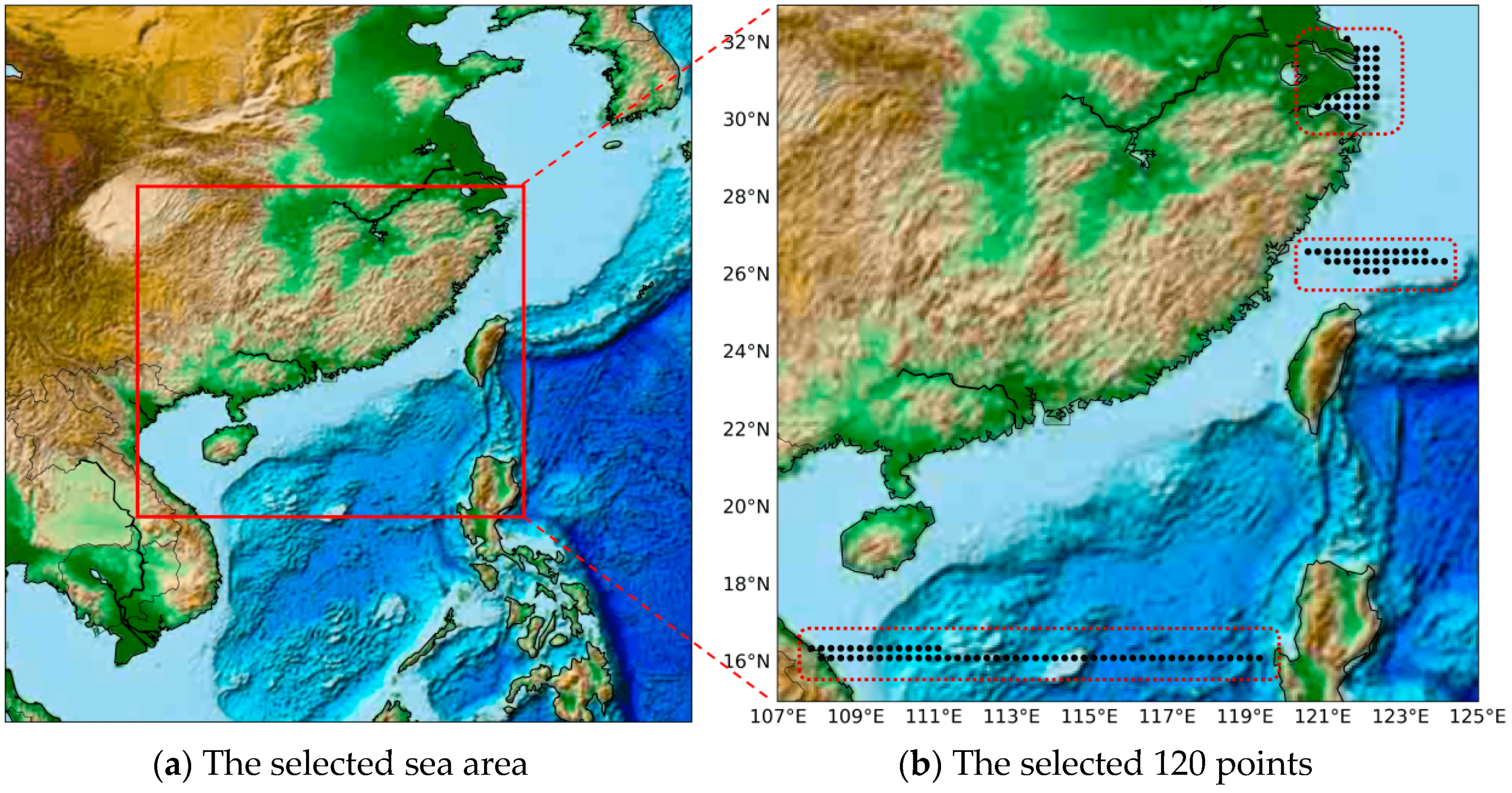
Wind data sets were extracted from the CCMP grid data in experiments covering the China Sea from 16° N to 42° N, 105° E to 127° E, as shown in Figure 4a. The experiment dataset was a gridded product with a spatial resolution of 0.25°, including the four major seas of China: the Bohai Sea, Yellow Sea, East Sea and South Sea. As shown in Figure 4b, we randomly selected 120 points from the entire experimental area (red dashed box). The temporal span of data was from January 2010 to April 2019, for a total of ten years. Because of the 6 h temporal resolution of the data, there were a total of 13,624 samples. We split the dataset into a training set (70%), validation set (10%), and test set (20%) in chronological order. The selection method and data in this paper were exactly the same as the main comparative baseline method STGN [21].

4.2. Setups

In this paper, we employed root mean squared error (RMSE) and mean absolute error (MAE) to evaluate our models, both of which are widely used in regression tasks. Specifically, assuming y i is the ground truth of ith node and y ~ i is the predicted value of ith node, where N denotes the number of nodes, they were defined as follows:
M A E = 1 N i = 1 N | y i y ~ i |
R M S E = 1 N i = 1 N ( y i y ~ i ) 2
M A P E = 100 % N i = 1 N | y i y ~ i y i |
In Equation (10), the MAE is the average of the absolute error between the true values and prediction values, which can reflect the overall prediction performance. The RMSE in Equation (11) is average of the square of the differences between the actual and predicted values. Compared to MAE, RMSE is more sensitive to values with large prediction errors in the data. For MAE and RMSE, lower values are better. In addition, when making a further comparison in the ablation experiment, we added mean absolute percentage error (MAPE) for observation, as shown in Equation (12). The closer the MAPE value is to 0%, the better the regression fit will be.
Implementation details. To demonstrate the good prediction performance of the model, experiments were conducted for both short- and long-term forecasts for wind speed prediction, with prediction scales of 6 h, 12 h, 18 h, 24 h (1 d), 48 h (2 d), 72 h (3 d), 96 h (4 d), 120 h (5 d), 144 h (6 d), and 168 h (7 d). Following the work of [20], the length of the time window was 12 and the step size was 1. We used the Adam optimizer [51] to train the wind speed prediction models. The batch size was 64 and the training epoch was 100. The learning rate started from 0.001 and the learning rate decay was ReduceLROnPlateau, where the patience was 20, the cooldown was 30 and the factor was 0.3. The CPU of the experimental device was i5-8400H, and GPU was NVIDIA’s GTX 1080 Ti. Our proposed method and model was implemented with pytorch-1.1.

4.3. Results and Analysis

We comprehensively evaluated the prediction performance of the proposed model AGLCN and eight other baseline methods based on wind datasets for the multi-scale prediction tasks. In order to have a fair and reasonable comparison, we used three types of baseline methods: (1) Methods that do not model multi-node spatial associations. (2) Non-graph structure methods that model multi-node spatial associations. (3) Modeling multi-node spatial associations using a predefined graph structure. Details of the baseline methods are described below.
Methods that do not model multi-node spatial associations. Wavelet-DBN-RF [52]: This model proposes a hybrid approach of deep learning and ensemble learning. It first decomposes the wind speed sequence using wavelet transform (WT) and extracts the high-dimensional features of the decomposed signal using a deep belief network (DBN). Each subsequence processed by the DBN is predicted using a light gradient boosting machine (LGBM) and random forest (RF). The experimental results show that the network improves the prediction performance of short-term wind speed prediction. DLinear [53]: This model decomposes the time series into trend series and residual series through a simple structure and uses two single-layer linear networks to extract the features of data.
Non-graph structure methods that model multi-node spatial associations. (1) PDCNN [31]: This work investigates the problem of predicting wind speed at multiple sites simultaneously and proposes a wind speed prediction model with a spatio-temporal correlation PDCNN. It integrates CNN and MLP to extract spatial features and temporal relationships, respectively. Experimental results show that the PDCNN outperforms traditional machine learning models. (2) CGRU [54]: This model uses both CNN and recurrent networks GRU to extract the spatio-temporal correlations of data. Experiments show a good performance on time series data. (3) TPA [55]: This work proposes a recurrent neural network with an attention mechanism. It uses RNN to extract temporal dependencies in multivariate time series data, while capturing unknown associations between variables using the attention mechanism. It achieves state-of-the-art performance on several real-world datasets.
Modeling multi-node spatial associations using predefined graph structures. (1) Multi-LSTMs [56]: This work models the spatio-temporal information in wind speed data through graphs and proposes a framework to obtain forecasts for all nodes in the graph simultaneously. Experiments on real wind power data demonstrate that the model improves short-term prediction performance. (2). SGNN [7]: This work constructs a graph structure of wind machines using geographic location information and proposes an SGNN (superposition graph neural network) for feature extraction. Experiments show that the method not only improves the prediction performance but also has good robustness. (3). STGN [20]: This paper proposes spatio-temporal correlation graph neural networks that use graph convolution and channel attention to capture spatial correlation in multi-node wind speed data. The graph structure is constructed based on geographical distance information.

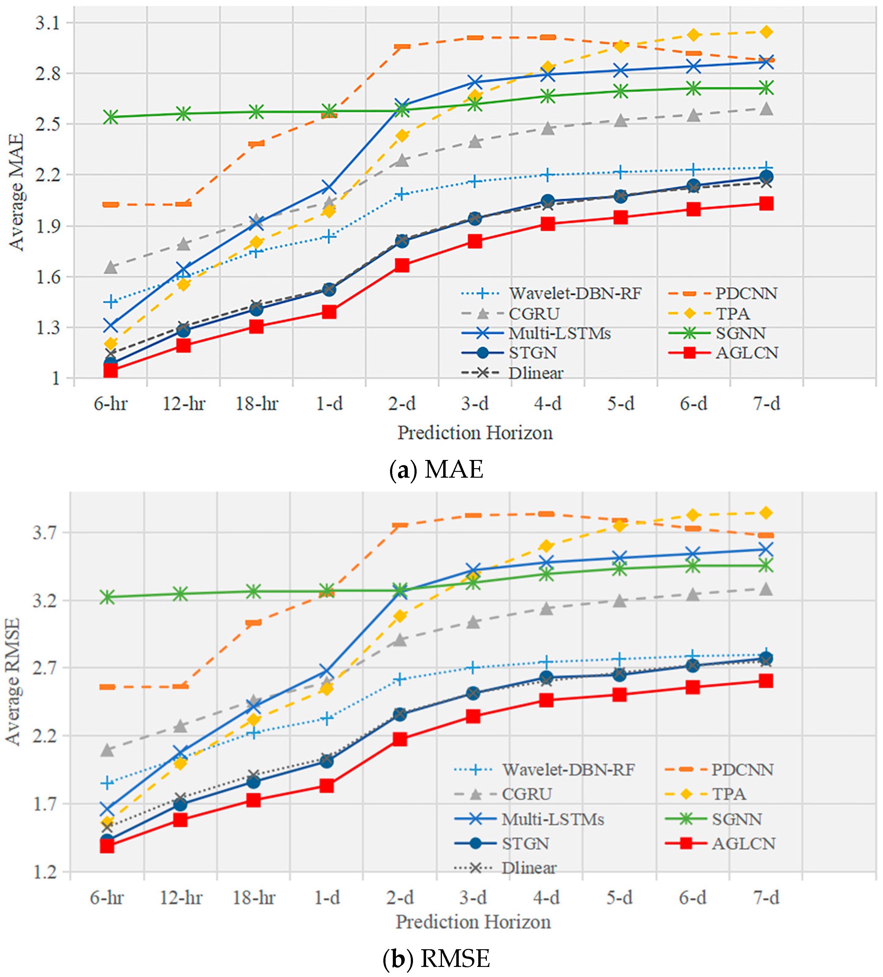
4.3.1. Comprehensive Comparison of Experimental Results

To verify the effectiveness of the proposed model by this paper, we conducted wind speed prediction experiments at multiple prediction scales and with different numbers of nodes. The overall prediction performances for wind speed, that are the averaged MAE and RMSE results for the 40-node and 120-node multi-scale wind forecasts, are shown in Table 1, Table 2, Table 3 and Table 4. The bold text in the table indicates the best prediction performance and underlining indicates the second-best prediction performance. Several observations from these results are worth highlighting:
(1)
Our method achieves the best prediction performance at all prediction scales of 40 and 120 nodes; the details are shown in Table 1, Table 2, Table 3 and Table 4. Compared to the best baseline method, STGN, our method improves by an average of 9% in MAE and RMSE for 40-node wind speed predictions and 6% in MAE and RMSE for 120-node wind speed predictions. Long-term prediction of wind speed is a challenging task due to cumulative error, but our method still maintains a good performance. For wind speed prediction at nodes 40 and 120, the 7-day prediction errors of MAE and RMSE of our AGLCN method are lower than the 3-day and 4-day prediction errors of STGN, respectively.
(2)
Methods that use attention mechanisms to model spatial associations (TPA) outperform the methods that use CNN (PDCNN, CGRU) and the methods that do not explicitly model spatial associations (Wavelet-DBN-RF) in short-term predictions (12 h). It shows that correct spatial modeling is effective. The important feature of CNN is translation invariance [57], yet for the complex spatial patterns of wind data, it is rather a bottleneck that limits the performance of the model. In long-term wind speed prediction (time horizon > 4-day), PDCNN and CGRU are better than TPA. The input time window is 12 and the forecast length is greater than 4-day (prediction length > 24). It means that the input data information no longer provides enough information to support the long-term forecasts. In this case, the attention mechanism approach, TPA, which relies entirely on the extraction of relationships from the data, is inferior to the relationship extraction approach with inductive bias, i.e., CNN (PDCNN, CGRU). DLinear are implemented based on a transformer and have excellent long-time-series prediction capability. Although they did not carry out spatial modeling for data, they still have a remarkable prediction ability. As a result, their performance exceeds STGN when under a long prediction scale but is still inferior to AGLCN.
(3)
Multi-LSTM and SGNN require a predefined graph structure to model spatial associations between multiple nodes. These two methods perform worse than the attention mechanism method, TPA, for the short-term prediction, but achieve better performance for the long-term prediction. Compared to Multi-LSTM, SGNN uses graph convolution operations, i.e., information propagation based on the graph, which also allows SGNN to achieve better results in long-term prediction. STGN basically achieves the second-best results (only worse than our AGLCN method) in both short- and long-term forecasting. The reason is that the model integrates the advantages of GNN and attention mechanisms.
In summary, attention mechanisms are effective at capturing relationships in the data for short-term forecasting, while graph structure plays an important role in long-term forecasting. Our AGLCN approach, on the other hand, constructs multi-node spatial correlations from an adaptive learned graph based on downstream tasks, achieving the best results in both short-term and long-term predictions, as shown in Figure 5. It demonstrates the power of the graph structure in modeling spatial associations and the effectiveness of the designed graph-learning approach. A further analysis of the learned graph structure can be seen in Section 5.
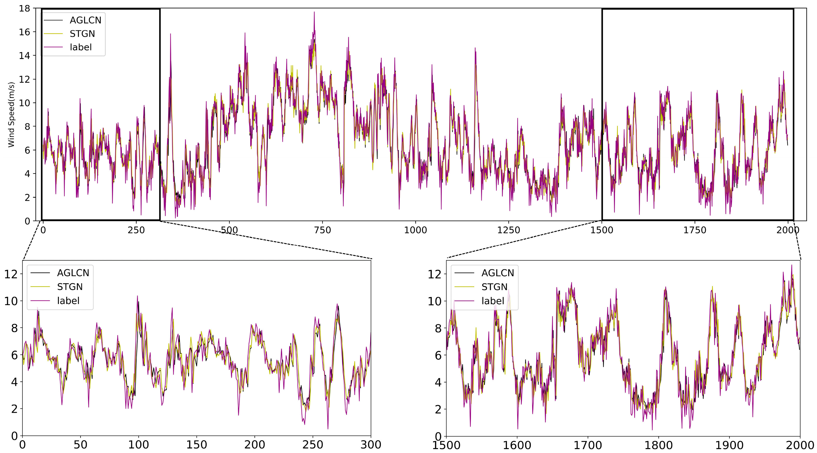
Figure 6 illustrates the visualization of the prediction results. Figure 6a presents the visualization using the best baseline method at 106 data points, while Figure 6b displays the visualization of our method’s prediction results at different scales. It is evident from Figure 6a that our method achieves more accurate prediction results. Additionally, Figure 6b shows that our method maintains a strong prediction performance across multiple scales. For further visualization of the prediction results, please refer to Figure A4 in Appendix A.

4.3.2. Hyper-Parameter Study

In this section, we present the hyper-parameter study of the proposed model and compare the detailed performance of the model under different hyper parameters.
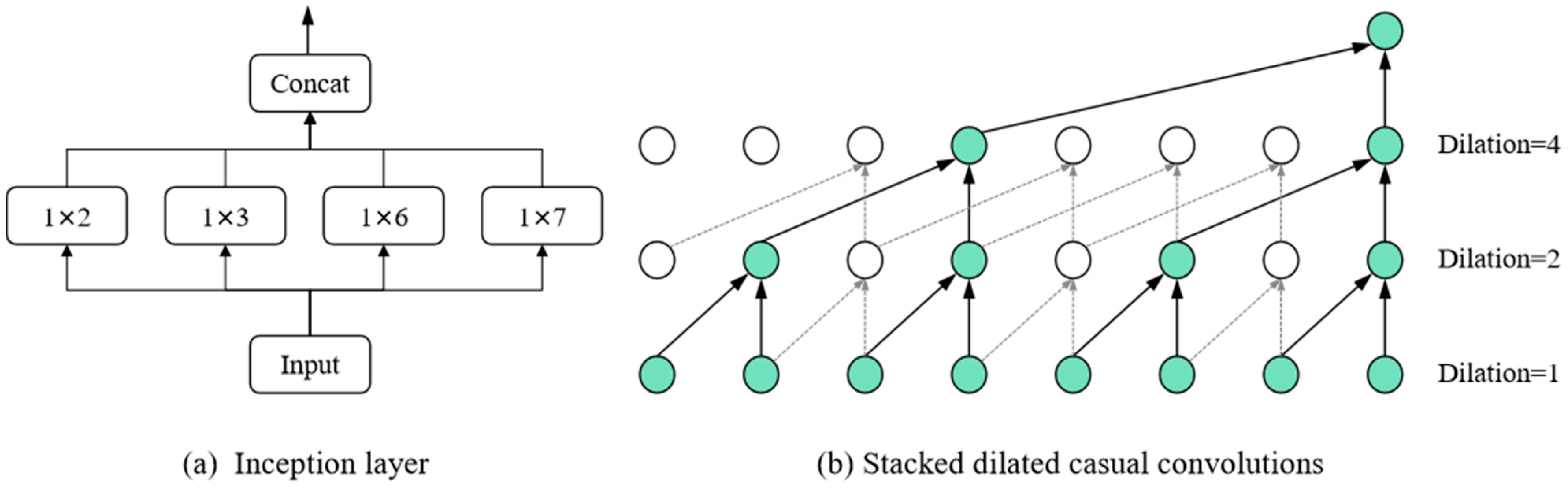
Table 5 shows the hyper-parameter search process for our proposed model, with the list of main parameters on the left, the search range in the middle, and the best hyper-parameter settings on the right. The number of channels refers to the channels in the TCN and GCN modules, K is the number of stacking layers of TCN and GCN, and d is dilation factor which determines the received field of the model. During the training process, the model was trained by the Adam optimizer with a gradient clip of 5. The learning rate decay was ReduceLROnPlateau, where patience was 20, the cooldown was 30, and factor was 0.3. The selection range for the following hyper parameters was as follows: the number of channels was [4, +∞], the number of layers of model K and dilation factor d was [1, +∞], the dimension of the node embedding was [1, +∞], the learning rate was (0, +∞]. The reason that the number of channels was at least four was that we conducted the convolution operation with four different convolution kernel size simultaneously in TCN, so the number of channels was preferably a multiple of four [47]. For the number of channels and the dimension of node embedding, too-small settings lead to a poor model-learning ability, while too-large settings lead to too many model parameters and thus an overfitting phenomenon. Together, the number of layers of the model and the dilation factor d determine the receptive field of the model. A receptive field that is too small will result in a model that does not take full advantage of the input data, while a receptive field that is too large will result in a model that is overfilled with zeros and affects performance. Thus, the general receptive field will be slightly longer than the length of the input window.
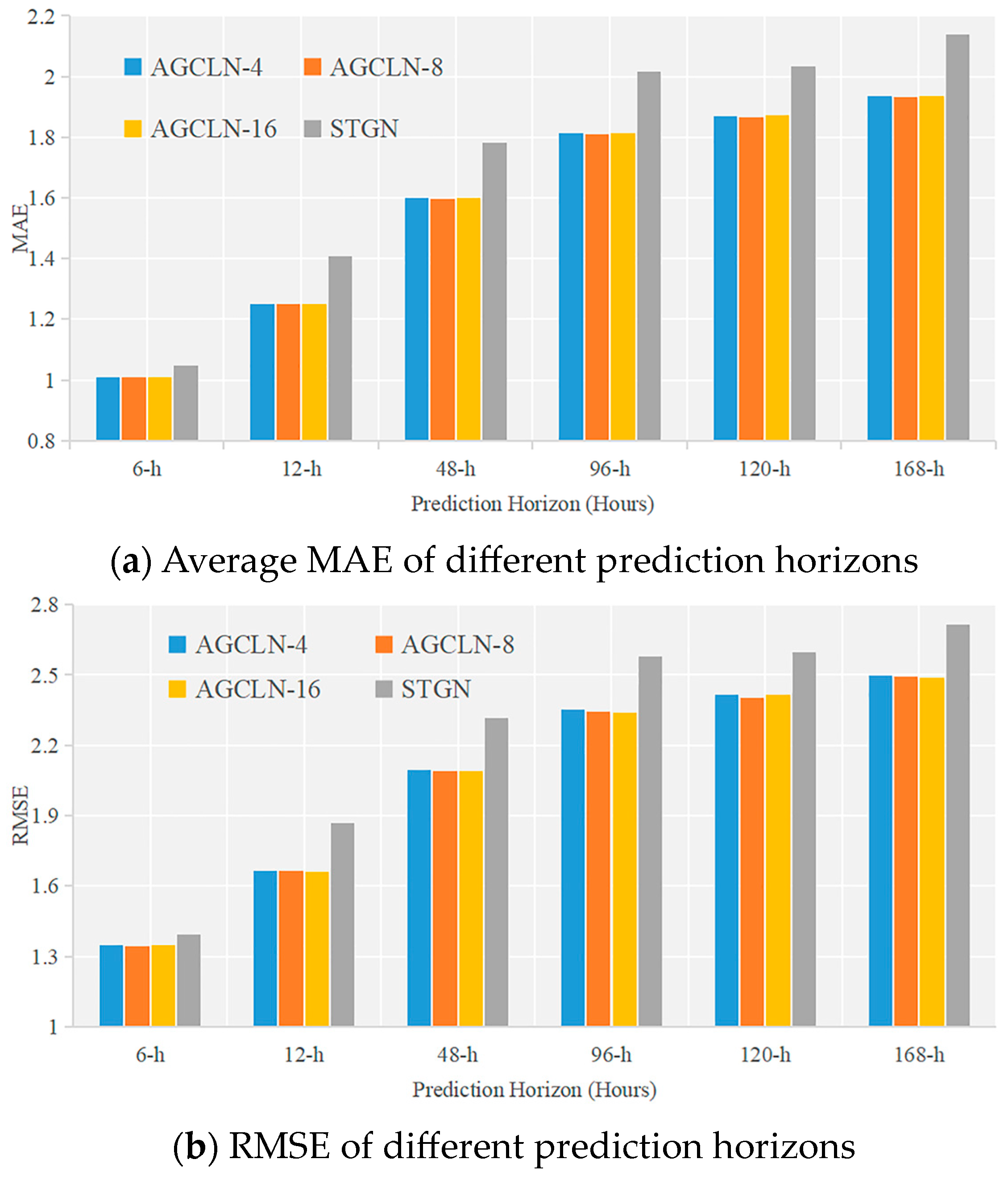
We first investigated the effect of the number of channels on the prediction performance of our model. Since we used four convolutions simultaneously in our temporal convolution (Equation (8)) to extract temporal dependencies, the number of channels was best set to a multiple of four. Here, we show experiments with three channel counts of 4, 8 and 16, as shown in Figure 7. To better show the effect of the number of channels on the performance, we have also included the model STGN, which achieved the best performance in the baseline approach, as a comparison. As shown in the figure, our model maintains a stable prediction performance for a different number of channels, all outperforming STGN. The larger number of channels represents more model parameters, but our model maintains excellent performance even with a small number of channels, demonstrating the validity of the model. On balance, we choose eight as the number of channels in the model.
Then, we investigated the effects of stacking layers K and dilation factor d on the model performance. The receptive field is jointly affected by the number of stacked layers and the dilation factor. When the dilation factor is equal to 1, it is a standard convolutional operation. Given the time window length 12, we conducted the four combinations (2,1), (2,2), (3,1) and (3,2) with receptive fields of 13, 19, 19 and 43, respectively, as shown in Table 6. When the receptive field was larger than the input time window, we padded the input with 0. As shown in Table 6, we can observe that our model maintains good performance for different combinations of stacking layers k and dilation factors d, all outperforming the baseline method STGN. Overall, the combination of (3,1) achieved the best results.
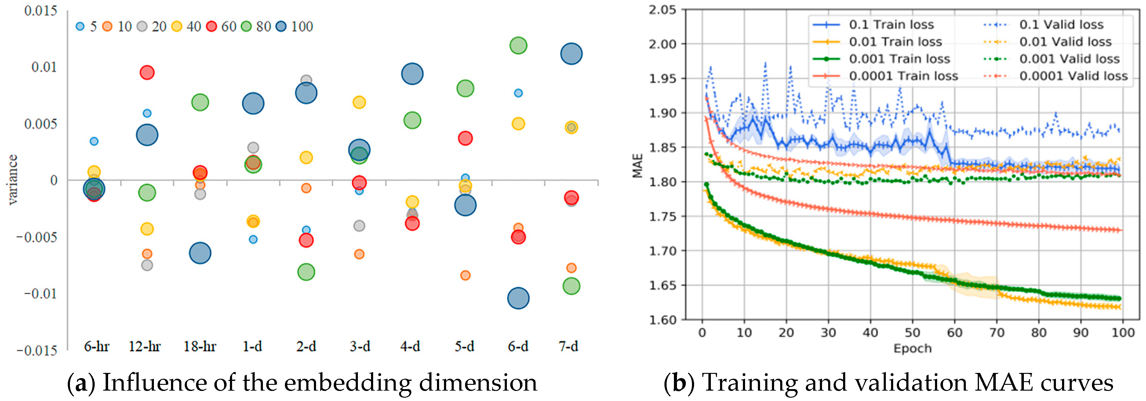
Here, we study the influence of the node-embedding dimension in our network. We find that the model AGLCN achieves good performance in all embedding dimensions. To better demonstrate the correlation between node-embedding dimensions and prediction performance, we counted the variance of different node-embedding dimensions. The result is shown in Figure 8a, where the horizontal coordinates are the prediction scales, the vertical coordinates are the variances, and the size of the circles represents the number of model parameters in different dimensions (the larger the dimension, the larger the number of parameters). The mean values of the RMSE for different node embedding dimensions at different prediction scales (6 h, 12 h, 18 h, 1 d, 2 d, 3 d, 4 d 5 d, 6 d, 7 d) are 1.345, 1.523, 1.660, 1.774, 2.090, 2.251, 2.334, 2.411, 2.456, 2.500 m/s. We can observe that our model also maintains a strong robustness in the node-embedding dimension, i.e., the node embedding expresses little correlation with the prediction performance (the variance random). Altogether, we set the node-embedding dimension to 10.
We visualized the training process of the models at different learning rates at 40 nodes as shown in Figure 8b, where the solid line represents the training MAE and the dashed line represents the validation MAE. We randomly initialized the seed and train of each model three times with the same optimizer and parameters. From the figure, we can see that the learning rate has a greater impact on the model compared to the other hyper parameters. Specifically, when the learning rate was 0.1, the learning rate was too large leading to difficulties in convergence and large fluctuations in both training and validation losses (blue curve). The best results for training and validation loss were achieved when the learning rate was 0.001 (green curve). At a learning rate of 0.01, there was a higher validation loss (yellow curve), and at a learning rate of 0.0001, the training and validation loss converged more slowly (tomato curve). These four learning rates (0.1, 0.01, 0.001, 0.0001) on the test set produced a MAE of 1.804, 1.744, 1.729 and 1.74 and a RMSE of 2.342, 2.264, 2.245 and 2.263.

4.3.3. Time Complexity

We analyzed the time complexity of the main components of the proposed model AGLCN, which is summarized in Table 7. Our model contains three main components, the graph-learning module, the graph convolution and the time convolution module. The graph-learning layer operations are focused on computing the graph matrix with time complexity O(N2M), where N denotes the number of nodes, and M represents the dimension of node embedding. Since we decoupled the information propagation and feature transformation operations in graph convolution, the main operation of graph convolution is the information propagation on the graph. The time complexity of the graph convolution layer was O(SN2D), where S represents the information diffusion step, N represents the number of nodes and D is the input dimension. The time complexity of the temporal convolution module equalled O(Nlcico/d), where l is the input sequence length, ci is the number of input channels, co is the number of output channels, and d is the dilation factor. The time complexity of the temporal convolution module mainly depends on N×l, which is the size of the input feature map.

4.3.4. Statistical Analysis

To ensure that the AGLCN can improve prediction accuracy, we conducted a statistical test [58]. Specifically, we utilized a paired two-tailed t-test to assess the predictive ability between the proposed AGLCN model and the baseline methods. The methods used an α = 0.05 significance level and were based on the “one-to-one” rule, i.e., we compared the AGLCN’s predicted values with the predicted values of other models one by one. Table 8 shows the statistical results of the paired two-tailed t-test. The results illustrate that our model has significant differences with the other state-of-the-art models. The statistical analysis proves that the forecasting performance of our model is superior to the other models at a 5% statistical significance level.

4.3.5. Ablation Study

To validate the effectiveness of our proposed key components, we conducted a series of ablation experiments on the different components of the model and carried out prediction with a prediction window of 6 h on 40-node datasets. AGLCN and its variants are defined as follows:
(1)
AGLCN-NE. In this variant, the graph-learning module is based on only the trainable node embedding.
(2)
AGLCN-DI. In this variant, the graph-learning module is based on only the dynamic node-level input.
(3)
AGLCN-PE. In this variant, we replaced the graph-learning module with the predefined graph structure.
(4)
AGLCN-SO. In this variant, we removed the softmax function of Equation (3) to demonstrate the effect of using the function to normalize the graph matrix.
The results of the ablation study are shown in Table 9. Compared to the AGLCN-NE and AGLCN-DI, a better performance is achieved for all information (node embedding and node-level input) considered, indicating the information fusion of the node embedding and input is important. The prediction performance of AGLCN is better than that of AGCLN-SO, which demonstrates the importance of using softmax in graph-learning methods. In fact, it is a popular practice to normalize the graph matrix using the softmax function [35,41]. The prediction performance of variants using predefined graph structures (AGCLN-PE) is worse than AGCLN, indicating the effectiveness of adaptive graph learning. Overall, it can be seen that the key components all contribute to the improvement of the proposed model.

4.4. Conclusions

To comprehensively demonstrate the validity of the proposed AGLCN, we performed validation on the real-world public CCMP V2.0 Wind Product. Detailed data descriptions and experimental settings are provided in Section 4.1 and Section 4.2. The experiment results on 40-node and 120-node multi-scale wind forecasts tasks proved the effectiveness of the proposed method, as detailed in Section 4.3.1. In addition, we used statistical analysis to ensure the superiority of the proposed approach compared to the baseline method, as detailed in Section 4.3.4. The hyper-parametric experiment in Section 4.3.3 proved that our method has good robustness. The detailed time complexity of each module of the model can be found in Section 4.3.3.

5. Discussion

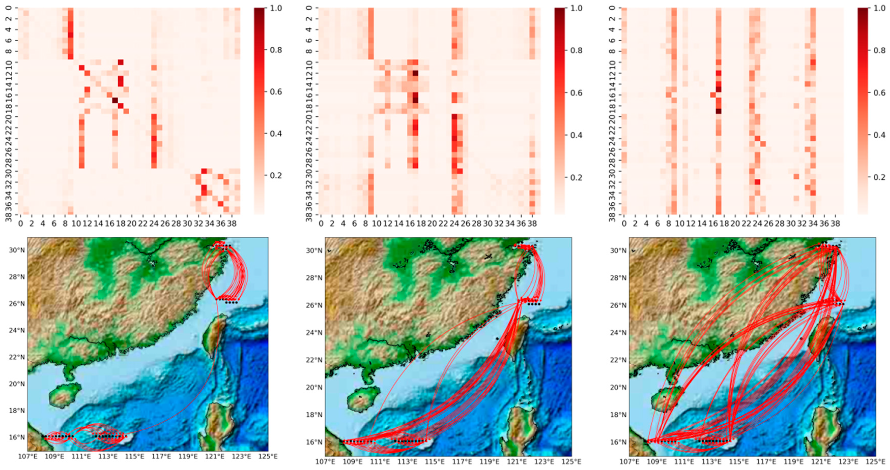
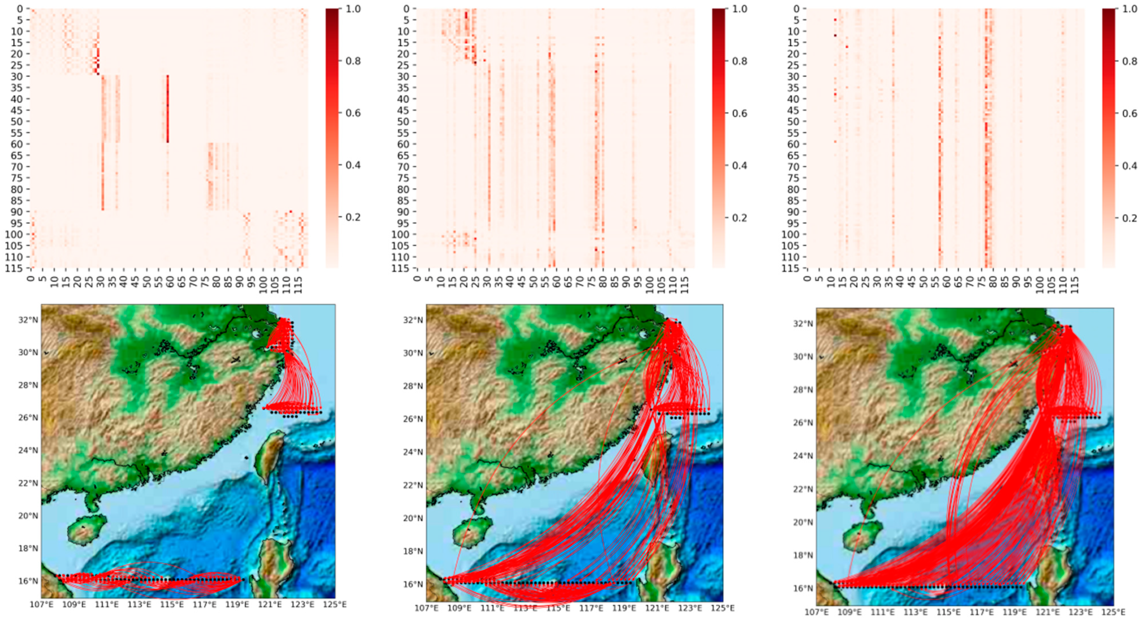
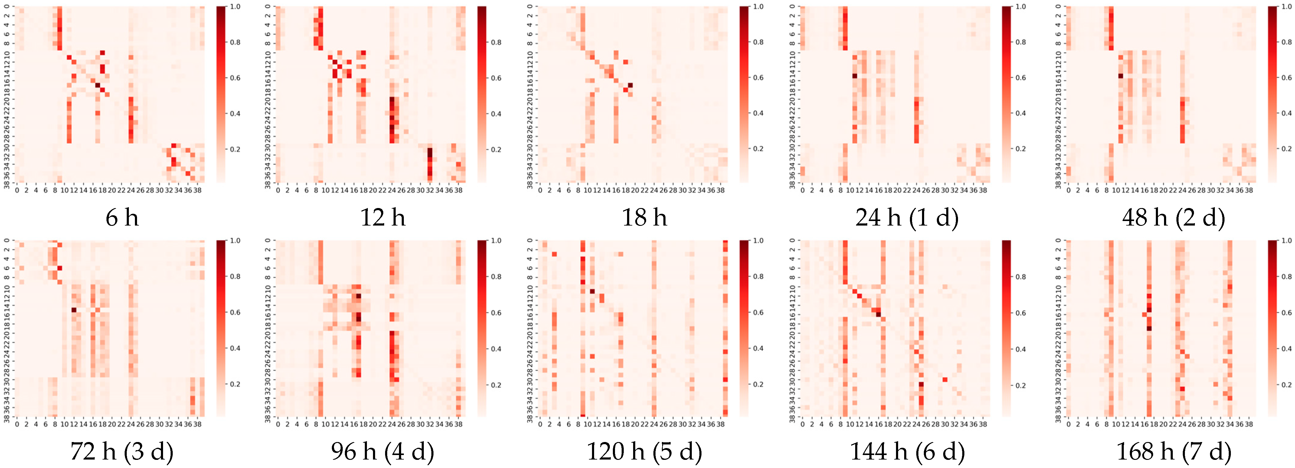
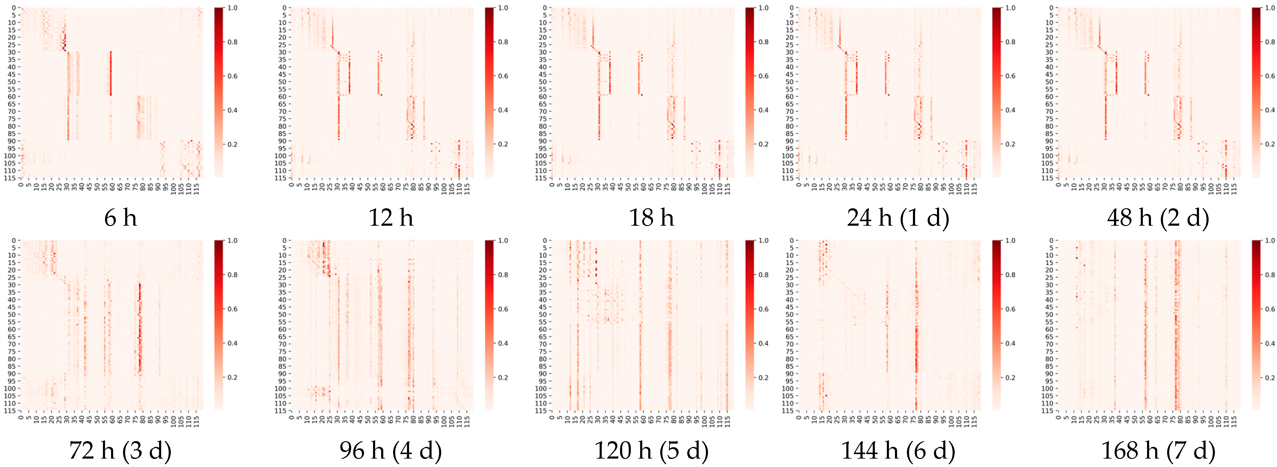
In this section, we visualize and analyze the graph matrix obtained by the model learning under different prediction scales, as illustrated in Figure 9 (For more detail, refer to Figure A1, Figure A2 and Figure A3 in the Appendix A). It represents the node associations captured adaptively at different prediction scales (6 h, 4-day and 7-day), where the heat map of the edge weights of the matrix is shown above, and we visualize the association on the actual map below for a better view. The shades of orange in the heat map represent the strength of the correlation between two wind speed points, including the correlations of the points with themselves. The horizontal and vertical axes, respectively, contain 40 points taken at different longitudes and latitudes, ordered from 0 to 40 in ascending order of latitude, or in ascending order of longitude if the latitudes are the same.
It can be observed that: 1. The graph structure is adaptively learned based on downstream tasks; 2. The graph structure can capture associations over long distances. Comparing the three heat maps in Figure 9, we can find that the learned graph structures are very different. The graph matrices obtained by our model are trained under different prediction scales independently, i.e., different downstream tasks. A more obvious local focus (i.e., the influence relationship is distance-dependent; the closer the distance, the greater the influence) is found in the heat map of Figure 9a; for example, the region where nodes 11–19, 32–39 are located shows a stronger association (darker colors). As the prediction scale is extended, we find that the local focus becomes weaker and weaker. For example, in the heat map in Figure 9b, the region where nodes 11–19 are located still shows a strong association, but the local focus in the region where nodes 32–39 are located has disappeared. In Figure 9c, the local focus has disappeared and only a few points are affecting the global nodes, i.e., a few very distinct vertical lines. This phenomenon is proved by projecting the edge weights from the heat map onto the real map. It is in line with practice, because the impact lagged in the process, so the influence of the surrounding nodes is greater in short-term forecasts. In the medium- and long-term forecasts, the influence between long distances gradually dominates, with the surrounding point effects still clearly observable in the 4-day forecast and long distance effects clearly dominating in the 7-day forecast. In medium- to long-term forecasting, our model captures long-range correlations well, free from the limitations of distance-based graphs.
It is important to note that the end purpose of this work is to improve forecasting performance using the adaptive learning graph, rather than identifying the causal relationship of the nodes. Inferring causality among multivariate time series requires a nontrivial extension that spans beyond the current study. A perfect golden and standard measure for the quality of the learned graph does not exist, except forecasting accuracy. In summary, our work demonstrates the ability to use adaptive graph structures for multi-node wind speed prediction and the potential to capture spatial dependence between nodes.

6. Conclusions

In this paper, we propose a general graph neural network framework for multi-node offshore wind speed named adaptive graph-learning convolutional networks (AGLCN). It aims to address the difficulty of existing methods to capture the unknown complex spatial dependencies between nodes and frees the need for an a priori graph structure. The proposed graph-learning method can automatically construct a graph structure based on dynamic wind speed data. To efficiently and effectively capture temporal dependencies in data, we employed a gated temporal convolutional network because of the parallel computational efficiency and gradient stability. We designed a general network framework AGLCN to integrate graph learning, as well as temporal and graph convolutional modules in a framework to jointly optimize these features. Experiments were conducted using real-world wind speed data from the China Sea, which demonstrated that our model achieved state-of-the-art results in all multi-scale wind speed predictions.
However, our SDGL has two potential limitations. The time complexity of the graph-learning method is O(N2), indicating that the computation cost grows quadratically with the number of nodes, which is not feasible in the face of large graphs with thousands of nodes. In addition, the spatial relationships between variables in the short-term view could differ from it in the long-term. Thus, we would like to further investigate these two topics in the future. Graph-learning methods with linear complexity will be studied to efficiently process large-scale graph nodes in the real world. Second, it is essential to learn multiple graph structures to capture the scale-specific spatial relationships among nodes.

Author Contributions

Conceptualization, J.L. and X.Y.; methodology, J.L.; software, X.Y. and Z.L.; validation, J.L., D.Z. and P.X.; formal analysis, J.L.; investigation, J.L.; resources, J.L.; data curation, X.Y.; writing—original draft preparation, J.L.; writing—review and editing, X.Y., D.Z., P.X. and F.H.; visualization, J.L.; supervision, D.Z.; project administration, F.H.; funding acquisition, D.Z. and F.H. All authors have read and agreed to the published version of the manuscript.

Funding

This paper was funded by the Science and Technology Department of Zhejiang Province (LGG21F020008), the National Natural Science Foundation of China (82011530399), the Zhejiang Provincial Natural Science Foundation of China (LGF21F020024), the key research and development program of Zhejiang (2021C01189), the Zhejiang Provincial Natural Science Foundation of China (LGG20F020015), the Natural Science Foundation of Zhejiang Province (LQ21F020025), the Science and Technology Department of Zhejiang Province (LGG21F020007) and the Leading talents of Science and Technology Innovation in Zhejiang Province (2020R52042).

Data Availability Statement

The data that support the findings of this study are produced by Remote Sensing Systems at https://data.remss.com/ccmp/v02.0/ (accessed on 2 February 2023), and the reference years are from 2010 to 2019.

Acknowledgments

We appreciate the Remote Sensing Systems the CCMP v2.0 data.

Conflicts of Interest

The authors declare no conflict of interest.

Appendix A. Visualization

Figure A1. The learned graph structure (120 nodes) at different prediction scales (from left to right 6 h, 96 h (4 d), and 168 h (7 d)).
Jmse 11 00879 g0a1
Figure A2. The learned graph structure (40 nodes) at different prediction scales, in order, 6 h, 12 h, 18 h, 24 h (1 d), 48 h (2 d), 72 h (3 d), 96 h (4 d), 120 h (5 d), 144 h (6 d), and 168 h (7 d).
Jmse 11 00879 g0a2
Figure A3. The learned graph structure (120 nodes) at different prediction scales, in order, 6 h, 12 h, 18 h, 24 h (1 d), 48 h (2 d), 72 h (3 d), 96 h (4 d), 120 h (5 d), 144 h (6 d), and 168 h (7 d).
Jmse 11 00879 g0a3
Figure A4. Comparison of the predicted results for wind speed at Point 1.
Jmse 11 00879 g0a4

Appendix B. More Ablation Study

Model architecture. They are currently divided into two main architectures, which are represented by DCRNN [48] and GraphWaveNet [42], respectively. The former combines GNN with recurrent neural network (RNN) to obtain spatial and temporal representations, respectively, while the latter uses a stacking convolutional neural network (CNN) instead of a recursive structure to improve training stability and efficiency. To demonstrate the effect of the model architecture on the predictive performance of multi-node wind speed, we combined the proposed graph-learning module with the DCRNN architecture. The predefined graph structure in the DCRNN was replaced with adaptive graph-learning method, and the results are shown as follows.
Table A1. The results of forecasting methods for 40 nodes.
Prediction ScaleDCRNN-AGLAGLCN
MAERMSEMAERMSE
6 h1.0211.3671.0081.344
12 h1.1871.6231.1381.517
18 h1.3491.8041.2471.659
1 d1.4051.9321.3341.771
2 d1.7222.1911.5962.090
3 d1.8832.3541.7292.245
4 d1.9482.4081.8102.342
5 d1.9942.4961.8652.403
6 d2.0422.5911.9062.452
7 d2.0672.5381.9332.493

Appendix C. More Study of Hyper Parameters

We conducted a parameter study on dropout, which influences the model performance, on the prediction window of 6 h on 40-node datasets. Dropout is a powerful method of regularizing a broad family of models to improve the generalization performance of the module, where the range is (0, 1]. Too small a value may lead to overfitting of the model, while too large a value may lead to underfitting of the model. The results are shown in Table A2. It indicates the best performance is achieved when dropout is 0.3.
Table A2. The prediction results of parameter study at 40 nodes.
6 hDropout
MAEMAPERMSE
0.11.04927.95%1.389
0.21.01227.36%1.367
0.31.00826.11%1.344
0.41.02926.81%1.351
0.51.05926.92%1.373
0.61.04927.18%1.398
0.71.06927.12%1.435
0.81.06427.13%1.421
0.91.08727.03%1.455

References

  1. Li, Y.; Chen, X.; Li, C.; Tang, G.; Gan, Z.; An, X. A hybrid deep interval prediction model for wind speed forecasting. IEEE Access 2020, 9, 7323–7335. [Google Scholar] [CrossRef]
  2. Wang, Y.; Li, Y.; Zou, R.; Foley, A.M.; Al Kez, D.; Song, D.; Hu, Q.; Srinivasan, D. Sparse heteroscedastic multiple spline regression models for wind turbine power curve modeling. IEEE Trans. Sustain. Energy 2021, 12, 191–201. [Google Scholar] [CrossRef]
  3. Hanoon, M.S.; Ahmed, A.N.; Kumar, P.; Razzaq, A.; Zaini, N.A.; Huang, Y.F.; Sherif, M.; Sefelnasr, A.; Chau, K.W.; El-Shafie, A. Wind speed prediction over Malaysia using various machine learning models: Potential renewable energy source. Eng. Appl. Comput. Fluid Mech. 2022, 16, 1673–1689. [Google Scholar] [CrossRef]
  4. Samadianfard, S.; Hashemi, S.; Kargar, K.; Izadyar, M.; Mostafaeipour, A.; Mosavi, A.; Nabipour, N.; Shamshirband, S. Wind speed prediction using a hybrid model of the multi-layer perceptron and whale optimization algorithm. Energy Rep. 2020, 6, 1147–1159. [Google Scholar] [CrossRef]
  5. Dong, Y.; Li, J.; Liu, Z.; Niu, X.; Wang, J. Ensemble wind speed forecasting system based on optimal model adaptive selection strategy: Case study in China. Sustain. Energy Technol. Assess. 2022, 53, 102535. [Google Scholar] [CrossRef]
  6. Wang, Y.; Wang, J.; Wei, X. A hybrid wind speed forecasting model based on phase space reconstruction theory and Markov model: A case study of wind farms in northwest China. Energy 2015, 91, 556–572. [Google Scholar] [CrossRef]
  7. Yu, M.; Zhang, Z.; Li, X.; Yu, J.; Gao, J.; Liu, Z.; You, B.; Zheng, X.; Yu, R. Superposition Graph Neural Network for offshore wind power prediction. Futur. Gener. Comput. Syst. 2020, 113, 145–157. [Google Scholar] [CrossRef]
  8. Liu, D.; Huang, Y.; Guo, J. Analysis and prediction on wind power in provincial grid. In Proceedings of the 2011 IEEE Power Engineering and Automation Conference, Wuhan, China, 8–9 September 2011; Volume 1, pp. 307–310. [Google Scholar] [CrossRef]
  9. Li, R.; Wang, Y. Short-term wind speed forecasting for wind farm based on empirical mode decomposition. In Proceedings of the 2008 International Conference on Electrical Machines and Systems, Wuhan, China, 17–20 October 2008; pp. 2521–2525. [Google Scholar]
  10. Li, H.; Jiang, Z.; Shi, Z.; Han, Y.; Yu, C.; Mi, X. Wind-speed prediction model based on variational mode decomposition, temporal convolutional network, and sequential triplet loss. Sustain. Energy Technol. Assess. 2022, 52, 101980. [Google Scholar] [CrossRef]
  11. Zhang, Z.S.; Sun, Y.Z.; Cheng, L. Potential of trading wind power as regulation services in the California short-term electricity market. Energy Policy 2013, 59, 885–897. [Google Scholar] [CrossRef]
  12. Soman, S.S.; Zareipour, H.; Malik, O.; Mandal, P. A review of wind power and wind speed forecasting methods with different time horizons. In Proceedings of the North American Power Symposium 2010, Arlington, TX, USA, 26–28 September 2010. [Google Scholar] [CrossRef]
  13. Xydis, G.; Koroneos, C.; Loizidou, M. Exergy analysis in a wind speed prognostic model as a wind farm sitting selection tool: A case study in Southern Greece. Appl. Energy 2009, 86, 2411–2420. [Google Scholar] [CrossRef]
  14. Monfared, M.; Rastegar, H.; Kojabadi, H.M. A new strategy for wind speed forecasting using artificial intelligent methods. Renew. Energy 2009, 34, 845–848. [Google Scholar] [CrossRef]
  15. Kosana, V.; Teeparthi, K.; Madasthu, S. Original article A novel and hybrid framework based on generative adversarial network and temporal convolutional approach for wind speed prediction. Sustain. Energy Technol. Assess. 2022, 53, 102467. [Google Scholar] [CrossRef]
  16. Furness, R.W.; Wade, H.M.; Masden, E.A. Assessing vulnerability of marine bird populations to offshore wind farms. J. Environ. Manage. 2013, 119, 56–66. [Google Scholar] [CrossRef]
  17. Klain, S.C.; Satterfield, T.; Sinner, J.; Ellis, J.I.; Chan, K.M.A. Bird Killer, Industrial Intruder or Clean Energy? Perceiving Risks to Ecosystem Services Due to an Offshore Wind Farm. Ecol. Econ. 2018, 143, 111–129. [Google Scholar] [CrossRef]
  18. Çevik, H.H.; Çunkaş, M.; Polat, K. A new multistage short-term wind power forecast model using decomposition and artificial intelligence methods. Phys. A Stat. Mech. Its Appl. 2019, 534, 122177. [Google Scholar] [CrossRef]
  19. Liu, X.; Lin, Z.; Feng, Z. Short-term offshore wind speed forecast by seasonal ARIMA—A comparison against GRU and LSTM. Energy 2021, 227, 120492. [Google Scholar] [CrossRef]
  20. Geng, X.; Xu, L.; He, X.; Yu, J. Graph optimization neural network with spatio-temporal correlation learning for multi-node offshore wind speed forecasting. Renew. Energy 2021, 180, 1014–1025. [Google Scholar] [CrossRef]
  21. Zhang, H.; Peng, Z.; Tang, J.; Dong, M.; Wang, K.; Li, W. Original article A multi-layer extreme learning machine refined by sparrow search algorithm and weighted mean filter for short-term multi-step wind speed forecasting. Sustain. Energy Technol. Assess. 2022, 50, 101698. [Google Scholar] [CrossRef]
  22. Candy, B.; English, S.J.; Keogh, S.J. A comparison of the impact of QuikScat and winds at wind vector products on met office analyses and forecasts. IEEE Trans. Geosci. Remote Sens. 2009, 47, 1632–1640. [Google Scholar] [CrossRef]
  23. Sun, W.; Gao, Q. Short-term wind speed prediction based on variational mode decomposition and linear-nonlinear combination optimization model. Energies 2019, 12, 2322. [Google Scholar] [CrossRef]
  24. Zhang, H.; Chen, L.; Qu, Y.; Zhao, G.; Guo, Z. Support vector regression based on grid-search method for short-term wind power forecasting. J. Appl. Math. 2014, 2014, 835791. [Google Scholar] [CrossRef]
  25. Mangalova, E.; Agafonov, E. Wind power forecasting using the k-nearest neighbors algorithm. Int. J. Forecast. 2014, 30, 402–406. [Google Scholar] [CrossRef]
  26. Wang, H.; Lei, Z.; Zhang, X.; Zhou, B.; Peng, J. A review of deep learning for renewable energy forecasting. Energy Convers. Manag. 2019, 198, 111799. [Google Scholar] [CrossRef]
  27. Elman, J.L. Distributed Representations, Simple Recurrent Networks, And Grammatical Structure. Mach. Learn. 1991, 7, 195–225. [Google Scholar] [CrossRef]
  28. Hochreiter, S.; Schmidhuber, J.U. Long Shortterm Memory. Neural Comput. 1997, 9, 17351780. Available online: https://direct.mit.edu/neco/article-abstract/9/8/1735/6109/Long-Short-Term-Memory?redirectedFrom=fulltext (accessed on 12 January 2023). [CrossRef] [PubMed]
  29. Liang, T.; Zhao, Q.; Lv, Q.; Sun, H. A novel wind speed prediction strategy based on Bi-LSTM, MOOFADA and transfer learning for centralized control centers. Energy 2021, 230, 120904. [Google Scholar] [CrossRef]
  30. De Liu, M.; Ding, L.; Bai, Y.L. Application of hybrid model based on empirical mode decomposition, novel recurrent neural networks and the ARIMA to wind speed prediction. Energy Convers. Manag. 2021, 233, 113917. [Google Scholar] [CrossRef]
  31. Zhu, Q.; Chen, J.; Zhu, L.; Duan, X.; Liu, Y. Wind speed prediction with spatio-temporal correlation: A deep learning approach. Energies 2018, 11, 705. [Google Scholar] [CrossRef]
  32. Kipf, T.N.; Welling, M. Semi-supervised classification with graph convolutional networks. In Proceedings of the 5th International Conference on Learning Representations, ICLR 2017, Toulon, France, 24–26 April 2017; pp. 1–14. [Google Scholar]
  33. Zhou, J.; Cui, G.; Hu, S.; Zhang, Z.; Yang, C.; Liu, Z.; Wang, L.; Li, C.; Sun, M. Graph neural networks: A review of methods and applications. AI Open 2020, 1, 57–81. [Google Scholar] [CrossRef]
  34. Bai, L.; Yao, L.; Li, C.; Wang, X.; Wang, C. Adaptive graph convolutional recurrent network for traffic forecasting. Adv. Neural Inf. Process. Syst. 2020, 33, 17804–17815. [Google Scholar]
  35. Seo, Y.; Defferrard, M.; Vandergheynst, P.; Bresson, X. Structured sequence modeling with graph convolutional recurrent networks. In Proceedings of the 25th International Conference, ICONIP 2018, Siem Reap, Cambodia, 13–16 December 2018; Volume 11301, pp. 362–373. [Google Scholar] [CrossRef]
  36. Yu, B.; Yin, H.; Zhu, Z. Spatio-temporal graph convolutional networks: A deep learning framework for traffic forecasting. IJCAI Int. Jt. Conf. Artif. Intell. 2018, 2018, 3634–3640. [Google Scholar] [CrossRef]
  37. Oord, A.V.D.; Dieleman, S.; Zen, H.; Simonyan, K.; Vinyals, O.; Graves, A.; Kalchbrenner, N.; Senior, A.; Kavukcuoglu, K. WaveNet: A Generative Model for Raw Audio. arXiv 2016, arXiv:1609.03499. [Google Scholar]
  38. Wang, Y.; Zou, R.; Liu, F.; Zhang, L.; Liu, Q. A review of wind speed and wind power forecasting with deep neural networks. Appl. Energy 2021, 304, 117766. [Google Scholar] [CrossRef]
  39. Cho, K.; Van Merriënboer, B.; Gulcehre, C.; Bahdanau, D.; Bougares, F.; Schwenk, H.; Bengio, Y. Learning phrase representations using RNN encoder-decoder for statistical machine translation. In Proceedings of the 2014 Conference on Empirical Methods in Natural Language Processing (EMNLP), Doha, Qatar, 25–29 October 2014; pp. 1724–1734. [Google Scholar] [CrossRef]
  40. Li, Z.; Yu, J.; Zhang, G.; Xu, L. Dynamic spatio-temporal graph network with adaptive propagation mechanism for multivariate time series forecasting. Expert Syst. Appl. 2023, 216, 119374. [Google Scholar] [CrossRef]
  41. Li, Z.L.; Zhang, G.W.; Yu, J.; Xu, L.Y. Dynamic graph structure learning for multivariate time series forecasting. Pattern Recognit. 2023, 138, 109423. [Google Scholar] [CrossRef]
  42. Wu, Z.; Pan, S.; Long, G.; Jiang, J.; Zhang, C. Graph wavenet for deep spatial-temporal graph modeling. IJCAI Int. Jt. Conf. Artif. Intell. 2019, 2019, 1907–1913. [Google Scholar] [CrossRef]
  43. Dauphin, Y.N.; Fan, A.; Auli, M.; Grangier, D. Language modeling with gated convolutional networks. In Proceedings of the 34th International Conference on Machine Learning, Sydney, Australia, 6–11 August 2017; Volume 2, pp. 1551–1559. [Google Scholar]
  44. Szegedy, C.; Liu, W.; Jia, Y.; Sermanet, P.; Reed, S.; Anguelov, D.; Erhan, D.; Vanhoucke, V.; Rabinovich, A. Going deeper with convolutions. In Proceedings of the 2015 IEEE Conference on Computer Vision and Pattern Recognition Workshops (CVPRW), Boston, MA, USA, 7–12 June 2015; pp. 1–9. [Google Scholar] [CrossRef]
  45. Yu, F.; Koltun, V. Multi-scale context aggregation by dilated convolutions. arXiv 2016, arXiv:1511.07122. [Google Scholar]
  46. Bai, S.; Kolter, J.Z.; Koltun, V. An Empirical Evaluation of Generic Convolutional and Recurrent Networks for Sequence Modeling. arXiv 2018, arXiv:1803.01271. [Google Scholar]
  47. Wu, Z.; Pan, S.; Long, G.; Jiang, J.; Chang, X.; Zhang, C. Connecting the Dots: Multivariate Time Series Forecasting with Graph Neural Networks. In Proceedings of the 26th ACM SIGKDD Conference on Knowledge Discovery and Data Mining Virtual Event, San Diego, CA, USA, 6–10 July 2020; pp. 753–763. [Google Scholar] [CrossRef]
  48. Li, Y.; Yu, R.; Shahabi, C.; Liu, Y. Diffusion convolutional recurrent neural network: Data-driven traffic forecasting. In Proceedings of the 6th International Conference on Learning Representations, ICLR 2018—Conference Track Proceedings, Vancouver, BC, Canada, 30 April–3 May 2018. [Google Scholar]
  49. Liu, M.; Gao, H.; Ji, S. Towards Deeper Graph Neural Networks. In Proceedings of the ACM SIGKDD International Conference on Knowledge Discovery and Data Mining, San Diego, CA, USA, 6–10 July 2020; pp. 338–348. [Google Scholar] [CrossRef]
  50. Atlas, R.; Ardizzone, J.; Hoffman, R.N. Application of satellite surface wind data to ocean wind analysis. Remote Sens. Syst. Eng. 2008, 7087, 70870B. [Google Scholar] [CrossRef]
  51. Kingma, D.P.; Ba, J.L. Adam: A method for stochastic optimization. In Proceedings of the 3rd International Conference on Learning Representations, ICLR 2015, San Diego, CA, USA, 7–9 May 2015; pp. 1–15. [Google Scholar]
  52. He, J.; Yu, C.; Li, Y.; Xiang, H. Ultra-short term wind prediction with wavelet transform, deep belief network and ensemble learning. Energy Convers. Manag. 2020, 205, 112418. [Google Scholar] [CrossRef]
  53. Zeng, A.; Chen, M.; Zhang, L.; Xu, Q. Are transformers effective for time series forecasting? arXiv 2022, arXiv:2205.13504. [Google Scholar] [CrossRef]
  54. Xu, L.; Geng, X.; He, X.; Li, J.; Yu, J. Prediction in Autism by Deep Learning Short-Time Spontaneous Hemodynamic Fluctuations. Front. Neurosci. 2019, 13, 1–12. [Google Scholar] [CrossRef]
  55. Shih, S.Y.; Sun, F.K.; Lee, H.Y. Temporal pattern attention for multivariate time series forecasting. Mach. Learn. 2019, 108, 1421–1441. [Google Scholar] [CrossRef]
  56. Ghaderi, A.; Sanandaji, B.M.; Ghaderi, F. Deep Forecast: Deep Learning-based Spatio-Temporal Forecasting. arXiv 2017, arXiv:1707.08110. [Google Scholar]
  57. Wiatowski, T.; Bolcskei, H. A Mathematical Theory of Deep Convolutional Neural Networks for Feature Extraction. IEEE Trans. Inf. Theory 2018, 64, 1845–1866. [Google Scholar] [CrossRef]
  58. Li, M.W.; Xu, D.Y.; Geng, J.; Hong, W.C. A hybrid approach for forecasting ship motion using CNN–GRU–AM and GCWOA. Appl. Soft Comput. 2022, 114, 108084. [Google Scholar] [CrossRef]
Figure 1. The workflow of the framework. (a) The workflow of a predefined graph. (b) The workflow of adaptive graph learning. First, the graph structure is inferred based on input and trainable node embedding. Then, the input and learned graph are entered into the temporal and graph convolution to extract a feature. Finally, the parameters of the model are optimized according to the prediction task.
Jmse 11 00879 g001
Figure 2. Workflow of AGLCN. First, the input X goes through the graph-learning layers to obtain the graph structure. Then, raw data X and the inferred graphs go through the TCN and GCN for feature transformation. The features extracted by the TCN at each layer are linked to the output module by skipping connections to obtain the prediction results. Finally, the network is jointly optimized via prediction loss and graph regularization. The number ①–⑤ mean the nodes of graph.
Jmse 11 00879 g002
Figure 3. (a) Inception layer. Multiple convolution kernels are used simultaneously in each layer for convolution operations. (b) Dilated casual convolutions with kernel size 2. With a dilation factor d, it picks inputs every d step.
Jmse 11 00879 g003
Figure 4. Experiment area.
Jmse 11 00879 g004
Figure 5. The performance in the multi-scale wind speed prediction on 120 nodes.
Jmse 11 00879 g005
Figure 6. Visualization of the prediction results.
Jmse 11 00879 g006
Figure 7. The performance of different channels on 40 nodes.
Jmse 11 00879 g007
Figure 8. The experiment of node-embedding dimension and learning rate at 40 nodes.
Jmse 11 00879 g008
Figure 9. The learned graph structure at different prediction scales (40-nodes).
Jmse 11 00879 g009
Table 1. MAE of forecasting methods for 40 nodes.
Prediction ScaleNo Spatial ModelingNon-GraphPredefined GraphGraph-Learning
Wavelet-DBN-RFDlinearPDCNNCGRUTPAMulti-LSTMsSGNNSTGNAGLCNImprovement
6 h1.3301.0981.9701.4031.0801.2201.9381.0481.0084%
12 h1.4971.2461.9711.5761.3631.5231.9471.2381.1388%
18 h1.6501.3602.2821.7541.5901.7491.9581.4091.24712%
1 d1.7411.4522.4271.8841.7591.9191.9681.5091.3348%
2 d2.0041.7142.6592.2632.2622.4211.9981.7811.5967%
3 d2.0861.8572.7762.3812.5772.6662.0221.9651.7297%
4 d2.1221.9352.8132.4472.9092.7972.0632.0151.8106%
5 d2.1401.9912.8192.4823.1942.8732.0942.0331.8656%
6 d2.1592.0342.8282.5323.4292.9252.1252.0931.9066%
7 d2.1652.0642.8452.5733.6532.9582.1432.1381.9336%
Table 2. RMSE of forecasting methods for 40 nodes.
Prediction ScaleNo Spatial ModelingNon-GraphPredefined GraphGraph-Learning
Wavelet-DBN-RFDlinearPDCNNCGRUTPAMulti-LSTMsSGNNSTGNAGLCNImprovement
6 h1.6931.4642.4491.7851.4051.5462.4621.3921.3443%
12 h1.9041.6722.4502.0181.7651.9312.4741.6381.5177%
18 h2.0911.8292.8522.2532.0512.2202.4881.8671.65911%
1 d2.1931.9933.0452.4242.2672.4312.5061.9891.77111%
2 d2.4952.2683.3712.8832.8693.0332.5402.3172.0908%
3 d2.5862.4053.5153.0403.2063.3352.5662.5252.2457%
4 d2.6252.5023.5413.0793.5533.4922.6192.5792.3426%
5 d2.6472.5613.5353.1123.8443.5812.6652.5982.4036%
6 d2.6712.6073.5393.1804.0733.6462.7082.6712.4526%
7 d2.6772.6423.5563.2274.2833.6892.7322.7172.4936%
Table 3. MAE of forecasting methods for 120 nodes.
Prediction ScaleNo Spatial ModelingNon-GraphPredefined GraphGraph-Learning
Wavelet-DBN-RFDlinearPDCNNCGRUTPAMulti-LSTMsSGNNSTGNAGLCNImprovement
6 h1.4511.1452.0251.6581.2031.3122.5421.0841.0454%
12 h1.5971.3062.0261.7951.5521.6452.5621.2811.1927%
18 h1.7491.4322.3851.9371.8031.9142.5731.4071.3057%
1 d1.8361.5282.5512.0381.9842.1292.5781.5231.3929%
2 d2.0871.8182.9592.2902.4322.6102.5831.8091.6678%
3 d2.1621.9473.0112.4012.6672.7482.6181.9421.8097%
4 d2.2002.0223.0122.4782.8362.7932.6662.0461.9115%
5 d2.2172.0802.9712.5252.9592.8182.6952.0731.9496%
6 d2.2322.1242.9182.5563.0272.8422.7122.1371.9986%
7 d2.2432.1552.8772.5943.0452.8672.7162.1892.0326%
Table 4. RMSE of forecasting methods for 120 nodes.
Prediction ScaleNo Spatial ModelingNon-GraphPredefined GraphGraph-Learning
Wavelet-DBN-RFDlinearPDCNNCGRUTPAMulti-LSTMsSGNNSTGNAGLCNImprovement
6 h1.8551.5282.5612.1001.5621.6633.2221.4301.3893%
12 h2.0381.7452.5622.2771.9972.0793.2461.6971.5827%
18 h2.2261.9133.0332.4612.3192.4153.2641.8631.7287%
1 d2.3282.0373.2432.5942.5442.6793.2702.0131.8349%
2 d2.6172.3663.7502.9113.0823.2573.2752.3582.1768%
3 d2.7032.5163.8243.0423.3833.4203.3282.5142.3457%
4 d2.7442.6043.8333.1413.5983.4773.3922.6312.4635%
5 d2.7662.6663.7893.1983.7453.5103.4312.6492.5045%
6 d2.7882.7213.7273.2453.8253.5403.4532.7172.5596%
7 d2.7982.7483.6753.2853.8423.5733.4582.7712.6065%
Table 5. Detail of hyper parameters.
Hyper-ParametersSearch RangeSelected Value
The number of channels{4, 8,16}8
K and dilation factor d{(2,1), (2,2), (3,1), (3,2)}(3,1)
Dimension of Node Embedding{5, 10, 20, 40, 60, 80, 100}10
Learning rate{0.1, 0.01, 0.001, 0.0001}0.001
Table 6. RMSE of forecasting methods of different K and dilation factor d for 40 nodes.
Prediction ScaleSTGN2 Layer 1 d2 Layer 2 d3 Layer 1 d3 Layer 2 d
6 h1.3921.35021.35191.34441.3543
12 h1.6381.52681.52391.51721.5226
18 h1.8671.66581.66041.65971.6574
1 d1.9891.77441.77331.77061.7755
2 d2.3172.09362.09422.09022.0877
3 d2.5252.25672.25872.24532.2478
4 d2.5792.34132.35792.34182.3642
5 d2.5982.43232.41682.40292.4137
6 d2.6712.46722.47772.45202.4586
7 d2.7172.51222.50092.49262.505
Table 7. Results of the time complexity analysis.
ComponentsTime Complexity
Graph-Learning LayerO(N2M)
Graph Convolution LayerO(SN2D)
Temporal Convolution LayerO(Nlcico/d)
Table 8. The results of the statistical tests.
Compared ModelsPaired Two-Tailed t-Tests
(Significance Level α = 0.05)
t-Statisticp-Value
PDCNN−28.5690.00000
CGRU−17.5640.00000
Wavelet-DBN-RF−15.3760.00000
Multi-LSTMs−27.4170.00000
TPA−23.3590.00000
SGNN−9.2870.00000
STGN−4.9620.00000
Dlinear−4.7430.00000
Table 9. The prediction results of the ablation study at 40 nodes.
Prediction ScaleAGCLN-PEAGCLN-DIAGCLN-NEAGCLN-SOAGLCN
MAEMAPERMSEMAEMAPERMSEMAEMAPERMSEMAEMAPERMSEMAEMAPERMSE
6 h 1.05126.59%1.4111.04626.63%1.4061.01426.74%1.3511.01426.86%1.3531.00826.11%1.344
12 h 1.19030.26%1.6001.18331.70%1.5801.13929.44%1.5191.14329.49%1.5211.13829.23%1.517
18 h 1.29633.82%1.7331.29934.44%1.7341.25132.18%1.6641.25131.95%1.6721.24730.98%1.659
1 d1.38035.17%1.8431.37234.69%1.8341.34134.11%1.7761.34334.79%1.7791.33434.17%1.771
2 d1.63442.02%2.2401.63042.31%2.2321.60441.52%2.1131.59940.59%2.1031.59640.13%2.090
3 d1.76046.12%2.2851.76145.10%2.2881.74245.36%2.2571.73345.33%2.2481.72945.08%2.245
4 d1.86249.33%2.4711.84548.61%2.4681.81947.91%2.3491.82647.78%2.3571.81047.56%2.342
5 d1.89150.30%2.4311.88448.69%2.4321.88149.65%2.4231.88648.15%2.4131.86547.96%2.403
6 d1.93350.62%2.4981.926849.91%2.4801.90848.90%2.4611.91349.56%2.4691.90648.37%2.452
7 d2.01151.13%2.5911.95651.47%2.5291.94750.15%2.5151.94049.70%2.5071.93349.67%2.493
Disclaimer/Publisher’s Note: The statements, opinions and data contained in all publications are solely those of the individual author(s) and contributor(s) and not of MDPI and/or the editor(s). MDPI and/or the editor(s) disclaim responsibility for any injury to people or property resulting from any ideas, methods, instructions or products referred to in the content.

