Article

A Case Study-Based Analysis of Uncertainties on the Assessment of Impulsive Underwater Noise for the Marine Strategy Framework Directive

1
Department National Noise Registry, Federal Maritime and Hydrographic Agency, Bernhard-Nocht-Str. 78, 20359 Hamburg, Germany
2
Müller-BBM Industry Solutions GmbH, 82152 Planegg, Germany
3
Department Marine and Freshwater Acoustics, ISPRA—The Italian National Institute for Environmental Protection and Research, Via Vitaliano Brancati, 48-00144 Rome, Italy
4
KTH Royal Institute of Technology, Teknikringen 8 plan 4, SE-100 44 Stockholm, Sweden
*
Authors to whom correspondence should be addressed.
J. Mar. Sci. Eng. 2023, 11(4), 847; https://doi.org/10.3390/jmse11040847
Submission received: 31 January 2023 / Revised: 31 March 2023 / Accepted: 3 April 2023 / Published: 17 April 2023

Abstract

:
The Marine Strategy Framework Directive (MSFD) has been an important driver for progress in monitoring and assessment of impulsive underwater noise in the marine environment of the European Union. An important achievement of the MSFD implementation was the development of regional noise registries, providing the data basis for assessments. Recently, the EU has made tremendous efforts to propose harmonized assessment approaches and first-of-their-kind regional quantitative thresholds for impulsive underwater noise. In light of these newly developed thresholds values, we analyze the suitability of the available data in the noise registries for assessment purposes under the MSFD and review sources of uncertainties regarding quantitative results. We present three regional case studies located in the North Sea, the Baltic Sea and the Mediterranean Sea. For each of these regions, a sound-intensive activity was selected that aligned with a realistic impulsive noise event reported for the region. We made use of available data in the noise registries and applied the EU Guidance recommended for the description of impulsive noise sources, but also used alternative approaches and observations as comparison. The case study analysis includes the evaluation of data availability, data quality and data accuracy in the noise registries, and identifies corresponding consequences of the data for the uncertainty and interpretability of assessment results, especially for the quantitative evaluation of habitat areas impacted by noise. Finally, we make suggestions for the improvement of the data basis in the noise registries and the optimization of the assessment accuracy.

1. Introduction

The impact of underwater noise on the marine environment has long been recognized as a significant risk to many habitats and their inhabiting species, especially with regard to intensive impulsive noise generating activities, most of which are already regulated within the European Union (EU) and other parts of the world. For EU Member States, the Marine Strategy Framework Directive (MSFD) promotes a sustainable use of the seas by requiring member states to achieve and maintain Good Environmental Status (GES). The EU acknowledged the importance of addressing the consequences of underwater noise input into the marine environment by including underwater noise as a specific descriptor for determining Good Environmental Status. The clear objective of the MSFD of introducing EU-wide threshold values on underwater noise for both impulsive and continuous noise served as a driver for the elaboration of the quantitative threshold values and the assessment framework for immediate implementation within all EU regions and sub-regions as adopted at EU-level at the end of 2022.
The focus of these newly established quantitative threshold values for impulsive underwater noise (low- and mid-frequency impulsive sounds, i.e., of short duration) under the MSFD lies on the maximum allowed proportion of an assessed habitat area that is affected or made unavailable due to disturbances by impulsive noise for both short and long-term exposure periods. This requires a determination of the spatial and temporal extent of noise exposure in habitats. Quantitative regional assessments under the EU MSFD are expected to make use of units of measurements as defined in criterion D11C1 of Commission Decision 2017 [1], given by the number of days per quarter (or per month if appropriate) with impulsive sound sources and the proportion (percentage) of unit areas or extent in square kilometres (km2) of assessment area with impulsive sound sources per year. For the comprehensive application of these newly established EU threshold values, the main causes for variations in the determined quantities which are to be assessed against quantitative threshold values must be understood.
The determination of disturbed habitat under the MSFD is based on biological criteria, i.e., species- or habitat-specific noise threshold levels. For this reason, mapping and quantifying habitat areas impacted by individual or cumulative impulsive noise sources as accurately as possible is essential for a reliable assessment result. For the estimation of the cumulative disturbed habitat areas, precise physical information about the noise source and its source location is needed, as well as sufficiently precise environmental information (e.g., oceanographic, geophysical, meteorological) for the estimation of the sound propagation. Only after these two prerequisites have been met is there a reliable basis for determining sound exposure at any given location. An assessment of sound impact on the marine environment can then be conducted using bioacoustics criteria. In three test cases presented in this study, uncertainties of the input data from the noise registries are investigated. The biological assessment basis as well as the modelling of sound propagation, which represent another source of uncertainty for assessment results, are not examined here.
As part of the implementation of the MSFD, regional noise inventories were established, with the cooperation of EU Member States and regional marine conventions since 2015, forming the common data basis across regions for the assessment of Good Environmental Status in relation to impulsive underwater noise. The data structure of these regional noise inventories was largely determined by the scientific guidance of the Technical Group on Underwater Noise (TG Noise). This group was established in relation to the Marine Strategy Framework Directive 2008/56/EC (MSFD) by the Directorate-General for the Environment (DG ENV) in 2010 and currently works under the direct mandate of the Marine Strategy Coordination group (MSCG). The group‘s work programme includes advice on monitoring and assessment methodologies and on the setting of threshold values as required by Commission Decision 2017/848/EU. The objectives for the establishment of the noise registries were, on the one hand, that technically relevant information on noise events would be collected, and, on the other hand, that by setting the lowest possible hurdles for reporting data, the highest possible participation of EU member states in this monitoring would be achieved. Hence, one of the most important successes of the introduction of regional noise registries was a transparent documentation of recorded anthropogenic underwater impulsive noise events in the EU marine areas, thus raising awareness of the cumulative risks of underwater impulsive noise for the marine environment. Since their implementation, the noise registries served to create a uniform and comparable basis for the collection of information on underwater impulsive noise events.
In order to reduce the minimum reporting requirements as much as possible and thereby motivate the most complete reporting of noise events, the TG Noise further recommended to provide the option of not reporting precise sound pressure levels, but to allow the use of specific noise level classes instead, which facilitates the reporting and allows for not disclosing sensitive and detailed information [2]. Unfortunately, this option has been adopted by Member States as the commonly used format for reporting events to noise registries. Therefore, the available information on sound levels usually does not go beyond the indication of level classes.
Current studies on the impact of underwater noise carried out within the framework of national Environmental Impact Assessments (EIA) are often very comprehensive and detailed, require high-quality data and often rely on results from in situ measurements. For the regional assessment under the MSFD, such extensive data are neither available and published in the regional noise registries, nor collected nationally in a standardized manner in all cases. Furthermore, a similar level of detail as for EIA seems inappropriate and infeasible for large-scale and long-term regional assessments subjected to the MSFD.
Nevertheless, the accuracy and quality of input data also plays an important role for the regional assessment of activity-related underwater impulsive noise emissions and the sound propagation into the marine environment. In light of the upcoming quantitative assessments for impulsive noise, urgent questions have to be addressed including the following: (1) Whether the existing database allows an assessment to be conducted for all EU marine regions for the current MSFD cycle? (2) What gaps exist in data coverage and what uncertainties arise based on the current data? (3) How to adjust at this stage to optimize the basis for the next cycle? (4) How to deal with insufficient data/degree of detail in the medium- and long-term to optimize the comparability and informative value of the assessments?
Here, we examine these issues using three highly relevant case studies for the assessment of impulsive underwater noise emanating from some of the most common and intense impulsive noise generating activities in Europe as recorded in the regional noise registries. We use the data available in the respective noise registries and apply recommendations of the TG Noise Monitoring Guidance 2014 [2,3,4] for the assessment of different impulsive noise generating activities.
In addition to a regional perspective of each of the three case studies, a specific technical focus was given to unique challenges of quantitative assessments. We examined (1) the uncertainty in deriving the exposed area due to source levels being provided in the form of level categories instead of precise values (case study in the North Sea), (2) the uncertainty in the derived exposed area due to source levels being provided with insufficiently representative metrics (case study in the Baltic Sea) and (3) the uncertainty in the assessment result for deriving noise impacts for noise events that are not included in the registry (case study in the Mediterranean Sea). Currently, such data gaps pose a particular challenge for existing registries regarding their role as data sources for quantitative assessments.

2. Materials and Methods

In this section, (1) the extent of information regarding impulsive noise events reported to the regional noise registries available for this study is briefly summarized, (2) the concept for the classification of source levels of reported impulsive noise events as proposed in the EU TG Noise technical guidance is reviewed and (3) the scope of the case studies is described.

2.1. Data Basis Available from Noise Registries

To analyze the extent and structure of assessment input data available in regional noise registries, we downloaded data from three publicly available regional databases that currently hold datasets on impulsive underwater noise. These databases were the ICES (International Council for the Exploration of the Sea) noise registry [5], containing impulsive noise data for the regions of OSPAR (Convention for the Protection of the Marine Environment of the North-East Atlantic) and HELCOM (Commission for the Protection of the Baltic Marine Environment); the INR-MED noise registry, which has been developed under the QUIETMED project [6], containing impulsive noise data for the Mediterranean Sea region; and the EMODnet Physics European Impulsive Noise Events Registry [7], containing subsets of data from different regions.
The impulsive noise events in the datasets downloaded from the platforms described above contain multiple parameters, such as information on the position and date of occurrence of an impulsive noise event, the type of noise generating activity causing the event and information about the source strength.
Importantly, the description of impulsive noise events within and between the regional datasets differs in terms of the resolution of spatial information on the source. The spatial information about the source position is defined either as a geographical point or by a rectangular polygon (also referred to as a grid cell). The size of the polygons is variable. For example, datasets in INR-MED contain rectangles of approximately 55 × 55 km in size, while EMODnet and ICES datasets use ICES statistical sub-rectangles with sizes of about 18 × 25 km (10′ lat × 20′ lon). Additionally, the ICES dataset contains rectangles of about 11 × 18.5 km in size. To indicate the spatial position of a noise event, it can be associated with such a predefined rectangle. This distributes the exact position of impulsive noise sources. While datasets retrieved from ICES and INR-MED provide information on source locations as geographic points and polygons, those retrieved from EMODnet provide information on source locations in the form of polygons only.
The time of the event occurrence is often indicated by a start and an end date with a temporal resolution of one day. A record may additionally contain the duration of the event with a temporal resolution of one second. The most simplistic temporal description used in the datasets specifies only the number of days per year containing impulsive noise events. In this case, a daily, monthly or quarterly assessment time scale is not possible.
The source strength of a noise event is described by different parameters depending on the dataset, such as the following:
  • The value code category: a number/category describing the noise source strength, e.g., EMODnet: 0–4; ICES, INR-MED: very low, low, medium, high, very high;
  • The source event type: a text describing the noise generating activity (e.g., explosion, airgun array, pile driving, etc.);
  • The application of technical noise abatement: a description if technical noise abatement was applied and, if yes, which technical solution was used.
The dataset retrieved from INR-MED and ICES included information on all three parameters, while EMODnet included information on the parameter of value code category only.
In the present work, the focus lies on the analysis of the available data downloaded from the regional databases. When utilizing these datasets for the purpose of regional quantitative assessments in combination with threshold values, it is important to bear in mind that available datasets represent only the reported amount of noise events within the different regions. The amount of unreported noise events may be significantly higher than the amount included in the datasets. Moreover, the available data do not allow for estimating of the number of missing events. Figure 1 summarizes the data completeness of parameters regarding the source event and the value code in the regional datasets retrieved for this study. The maximum data completeness with respect to the source event parameter is 100% for all regional datasets of databases containing this parameter (i.e., ICES and INR-MED). EMODnet does not include any information on the source event. The data completeness of parameters in relation to the value code category varies from approx. 80% to 100%. Some of the missing value code entries likely arise from noise events related to military operations, where this information was deliberated omitted. Other entries are missing for unknown reasons.
For more than 20% of the available data in the ICES dataset, no information about the value code category is available. Further, numerous events are only associated with the source information of the polygon type. Exact source levels were only available in rare cases. Furthermore, there is no information about the spectral distribution of the sources, which, however, have a significant influence on sound propagation. For a more detailed overview of the available information in the regional datasets regarding the source strength, the number of reported impulsive noise events associated with value codes was calculated for each year in the period between 2008 and 2019. The results of the statistical evaluation of the available information on the value code categories describing the source strength of impulsive noise events for all three regional datasets are shown in Figure A1, Figure A2 and Figure A3 in Appendix A.

2.2. Review of the Classification of Source Levels According to EU TG Noise Guidance

In the following, the concept for the classification of source levels of reported impulsive noise events as proposed in technical guidance from the EU is summarized and reviewed. The current classification and categorization of noise sources proposed by the EU TG Noise [2,3,4] and implemented in the structure of the regional noise registries is summarized in Table 1 and Table 2. Three overall noise type categories are distinguished as detailed in Table 1: (1) multiple impulsive noise events such as those produced by pile driving and air guns; (2) single events such as explosions; and (3) continuous sound events such as sonars. Five noise generating activity types were distinguished for reporting purposes, and different physical quantities were defined for practical reporting, as described in Table 2.
The value code categories have lower and upper class boundaries, which are not evenly distributed. Therefore, the class sizes vary from 24 dB ranges to 10 dB ranges. According to the classification described in [4,8,9], an event with a SEL of 140 dB re 1 µPa2s to 164 dB re 1 µPa2s for a multiple impulsive source and an event with a SEL of 164 dB re 1 µPa2s to 188 dB re 1 µPa2s for a single impulsive source (explosion) are both categorized in the value code category “very low”. When comparing reported events of different source types with each other, the metrics and thresholds vary even within the same value code category. Therefore, weighting (depending on the duration and intensity of the source event) is implicitly applied at this stage, even without considering any regional or species-related weighting criteria.
For the assessment of multiple impulsive source events and non-pulse sounds, the biological threshold values above, which include impulsive noise sources in the noise registry and correspond to the lowermost value code categories, were derived from studies on the onset of disturbance in marine mammals. For explosions, the onset of TTS in marine mammals was considered as the biological threshold value above which impulsive noise sources are included in the noise registry.
The threshold values considered as the basis for the inclusion of events into the noise registry were defined so as to apply to a location at a distance of 1000 m to the source, and were then converted to a monopole energy source level with a propagation loss (valid for shallow water) of 46 dB, as listed in Table 1. The monopole energy source level, also called energy source level or sound exposure source level re 1 µPa2m2s, is equal to the sound exposure level re 1 µPa2s in a specified direction at a distance of 1 m from a hypothetical point source located in a (hypothetical) infinite, uniform, lossless medium, as described in ISO 18405 [10].
It is worth recalling that the basis for the classification of sound sources should correspond to a monopole sound source level according to the Commission Decision of 2017 [1]. It is important to note that there are no national or international standards describing how to determine a monopole sound source level from underwater measurements. Therefore, it must be assumed that the classification (Table 1 and Table 2) is subject to additional uncertainties, the degree of which cannot be estimated.
For pile driving noise, the TG Noise has developed a first revision proposal that allows the use of in situ measurement data for the classification of noise events [11,12]. Table 3 shows the classification of source levels into the proposed noise class revision based on in situ measurements of SEL, Lp,pk (zero-to-peak sound pressure level) or hammer energy. The value type classification according to Table 3 was used for the analysis of uncertainties in this case study.
Due to the established databases providing the possibility of using reported in situ measurement data, the application of technical noise abatement measures can be used for the purpose of event value code categorisation. An international standard for these in situ measurements is available in ISO 18406 [13].

2.3. Scope of the Case Studies

For the North Sea region, pile driving activities were studied as a test case scenario for a regional assessment of impulsive underwater noise. Particularly because of ambitious expansion targets for renewable energies in many marine regions of the European Union, these noise events are among the most frequent ones that occurred in the past and will occur in the coming years. For this construction technique, long steel piles are driven into the seabed by repeated hammer blows to support offshore structures. The impulsive noise induced in the water column and seabed is an unintended side effect of this construction activity. These acoustic emissions are known to reach levels that may cause not only disturbance but also injury to several marine species over considerable large areas. The technical focus for the North Sea pile driving case study was to evaluate uncertainties to be expected when determining exposed areas based on the data available in noise registries, and to identify and develop proposals to reduce these uncertainties. This technical focus was identified as highly relevant with respect to the quantitative regional evaluation of fractions of habitats that exceed a tolerable noise exposure condition (e.g., to assess the compliance with threshold values as required on EU level). Although results in this subsection relate to a pile driving event in the North Sea, the general findings apply to all marine regions and noise sources.
For the Baltic Sea region, an underwater explosion event was selected as a test case scenario. Due to the presence of munitions waste in the seas, among other factors, explosion incidents are unfortunately still a common type of impulsive noise event, with a high potential for damage to the marine environment. Furthermore, the prediction of noise emissions from explosion events is complex and the quantitative estimation of the impulsive noise depends on numerous factors. Hence, the technical focus for the Baltic Sea explosion case study was placed on the (spectral) description of the source as input data for the evaluation of effect ranges and exposed habitat areas. An important target for this case study was to propose a pragmatic description of the source that nevertheless realistically represents sound emissions in this test case and provides the opportunity for a measurement-based verification.
For the Mediterranean Sea region, a seismic airgun survey was selected as a test case scenario. For the regional assessment of impulsive sound in the Mediterranean Sea, not only does the high complexity of the ocean environment have to be taken into account, but also the large number of sound-sensitive species and their variable habitats. The technical focus of this case study was on the procedure of combining physical and biological input data in the form of habitat areas, thus moving from exposed area to exposed habitat, as well as the presence of data gaps in the noise registry.

3. Results

In these subsections, an analysis of the current data content of regional noise registries is presented and potential uncertainties in the determination of the exposed area due to the structure and extent of the input data are illustrated by means of the case studies.

3.1. Case Study: Pile Driving Activities in the North Sea

We recall that information on the source level of impulsive noise from pile driving is reported according to the value code categories as described in Table 1, Table 2, and Table 3. We define our case study event to represent a hypothetical pile driving event in the North Sea reported with a value code category of “low”, corresponding to a SEL of 162–171 dB re 1µPa2s in a distance of 750 m from the source location (cf. Table 3).
The propagation loss versus distance for our hypothetical pile driving event in the North Sea reported with a value code category of “low” was estimated using the frequency dependent transmission loss (TL) equations empirically derived for different regions of the North Sea by Thiele and Schellstede [14], which can be written as follows:
T L = 16.07 + 0.185 F ( log R + 3 ) + 0.174 + 0.046 F + 0.005 F 2 R .
Here, R denotes the distance to the source in kilometers and the logarithm of the frequency grid point is given by F = 10 log10(𝑓/1000) with the frequency 𝑓 in Hertz. Results for the propagation loss versus distance are depicted in Figure 2, with the propagation loss curve corresponding to the upper bound in green and to the lower bound in blue, respectively, in the range defined for the value code category “low”. As additional criteria for the estimation of the exposed area due to our event, we defined a significance threshold value as SEL of 140 dB re 1µPa2s, which determined which area was interpreted as being adversely affected. This significance threshold was applied in this study, as it was used to define the lowermost biological relevance limit of event source strength, which has to be reported to the regional noise registries (TG Noise Guidance Part 2 and 3) [3,4]. This lowermost biological relevance limit was derived from results on the noise sensitivity of the Harbour Porpoise (Phocoena phocoena).
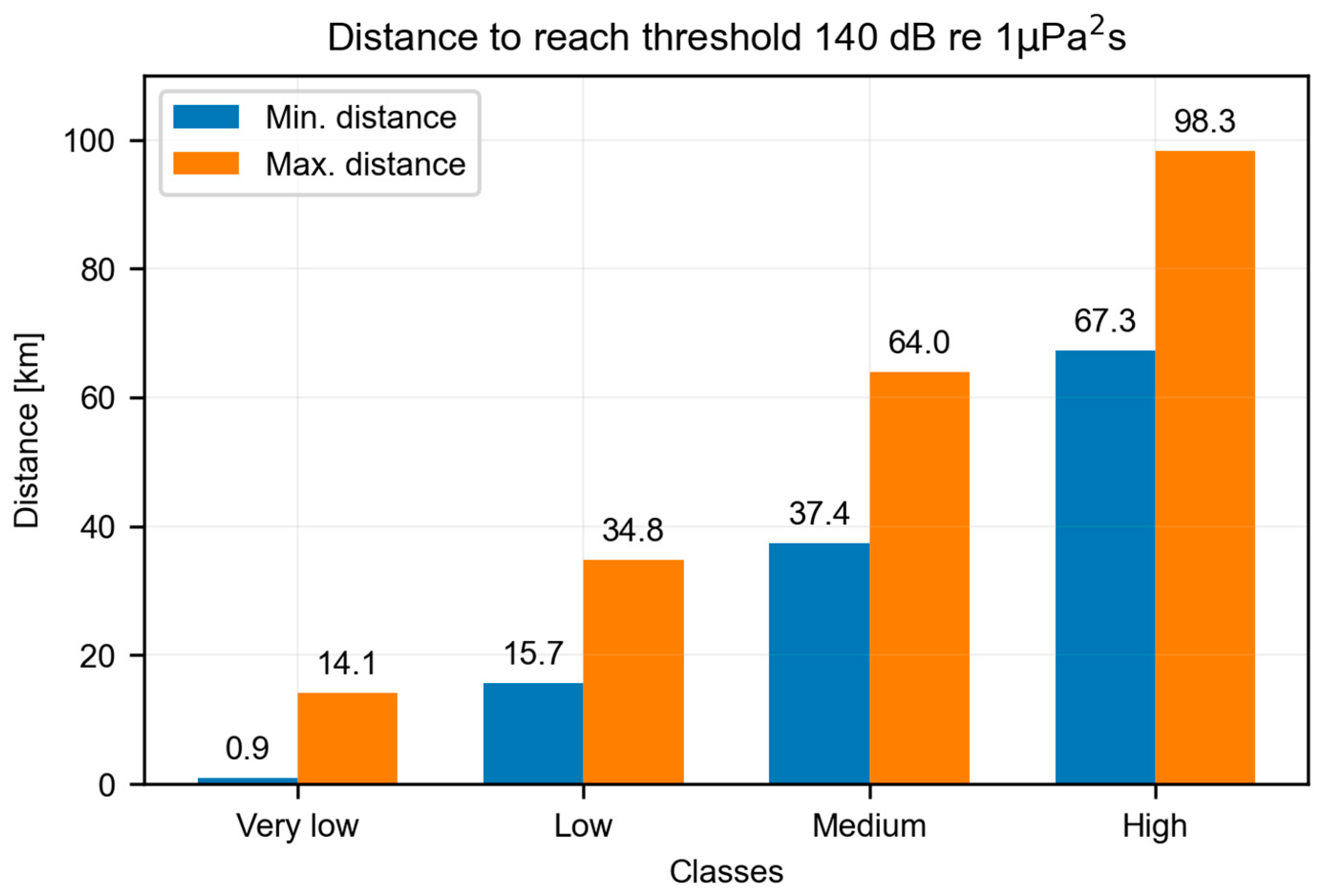
The propagation distance to reach SEL of 140 dB varies between 15.7 km (for the initial value of 162 dB) and 34.8 km, which implies a difference of 19.1 km of uncertainty within the same class. When using the value code categories to determine the exposed area, large uncertainties occur due to the class ranges.
Figure 3 shows the distances to reach a threshold of 140 dB for all value classes of impact pile driving. It is directly evident that considerable uncertainty exists in determining the exposed area when information on noise classes is not available. However, even when information on noise classes is available, uncertainty in the exposed areas determined can be relevant, as summarized in Figure 4 and Table 4.
Further, we quantified realistic uncertainties resulting from the available information on source locations. Data to the ICES Noise Registry can be reported using the exact location of an impulsive noise event (coordinates) or an attribution to corresponding geographic polygons, such as ICES Sub rectangle or UK License Block [5]. The exact source position of pile driving events is commonly reported to noise registries. However, the following analysis is also representative for uncertainties in source locations for other event types. Modelling of sound propagation based on source coordinates using impact areas or propagation formulas results in an accurately derived exposed area, apart from uncertainties in the propagation calculation itself. Events reported as ICES sub-rectangles (approximately 18 km × 25 km in size) or UK license blocks do not provide information on the exact location. Figure 5 presents different ways of handling the definition of possible locations of an event inside a sub-rectangle, for which the true location within the rectangle remains unknown. If the polygon edges (Figure 5 top left) are used as a worst-case assumption of an otherwise spatially undefined source location, results for the exposed area can be overestimated. The effects of the choice of the event location within the sub-rectangle on the affected area and the uncertainties derived from this will be quantified in the following paragraphs.
Instead of using propagation modelling to determine the area exposed with received noise levels above a biological effect level, the calculation of exposed areas may be based on predefined effect ranges (distance of effect) [15] derived from observations, e.g., 12 km for mitigated pile driving and 20 km for non-mitigated pile driving, without taking noise classes into account. Consequently, quantitative results of exposed area will deviate between these approaches, which must be considered in impulsive noise assessments.
If the exact location of the event is not available, but only the grid cell information, assumptions must be made about the source location to determine the exposed area. As an example, we selected four possible configurations depicted in Figure 5 and calculated the corresponding exposed areas. Results are presented in Figure 6. It can be concluded that the choice of the source location decisively determines the exposed area. In our example, the exposed fractions of the considered areas range between 4 and 10%, with respect to the area of the southern North Sea. These uncertainties need to be taken into account for a quantitative regional assessment using threshold values. If areal blocks have to be used as spatial input data, a standardization of the assessment could be represented by a worst-case scenario (according to the precautionary principle), where all locations in a polygon are set as source location. If value code classes have to be used for the estimate of source levels, a worst-case scenario could imply that the upper range of the value code level classes is used as source level. However, from a statistical point of view, the use of such worst-case approaches would lead to significant overestimations of exposed areas. We suggest preventing this by instead aiming at more detailed input data, which is verified by in situ measurements.

3.2. Case Study: Underwater Explosion Event in the Baltic Sea

In the second case study, we focus on examining different input data to describe the noise source and its impact on the results for estimating noise exposed habitat areas. Our case study in the Baltic Sea concerns an underwater explosion, which occurred in the Stockholm Archipelago. A measurement campaign using explosion trials was performed in this region between April and May 2015 with TNT equivalent charge masses of 105 kg [16] detonated in variable water depth. These impulsive noise events were reported to the regional noise registry for the Baltic Sea (ICES) without disclosing the exact location of the events. The ICES noise registry contains several events of source type explosion in this region with information on the event date and the ICES sub-rectangle in which the source is located. These events were reported as explosions of the value code category “high”. The explosions were recorded by multiple hydrophones located at different depths (20 m, 30 m, 50 m) and distances to the source towards the coast in the vicinity of the marine protection area (MPA) Huvudskär, a nearby Nature2000 site for grey seals (Halichoerus grypus). Table 5 summarizes a selection of the available measurement data as published in [16]. The exact positions of the measurements are, however, not known to the authors of this study.
In addition to information on the measurements as published in [16], we made use of publicly available information for the bathymetry with a maximum resolution of approximately 40 m × 40 m retrieved from EMODnet bathymetry [17]. The spatial information for the extent of the marine protection area Huvudskär was retrieved from Natura 2000 datasets [18]. 
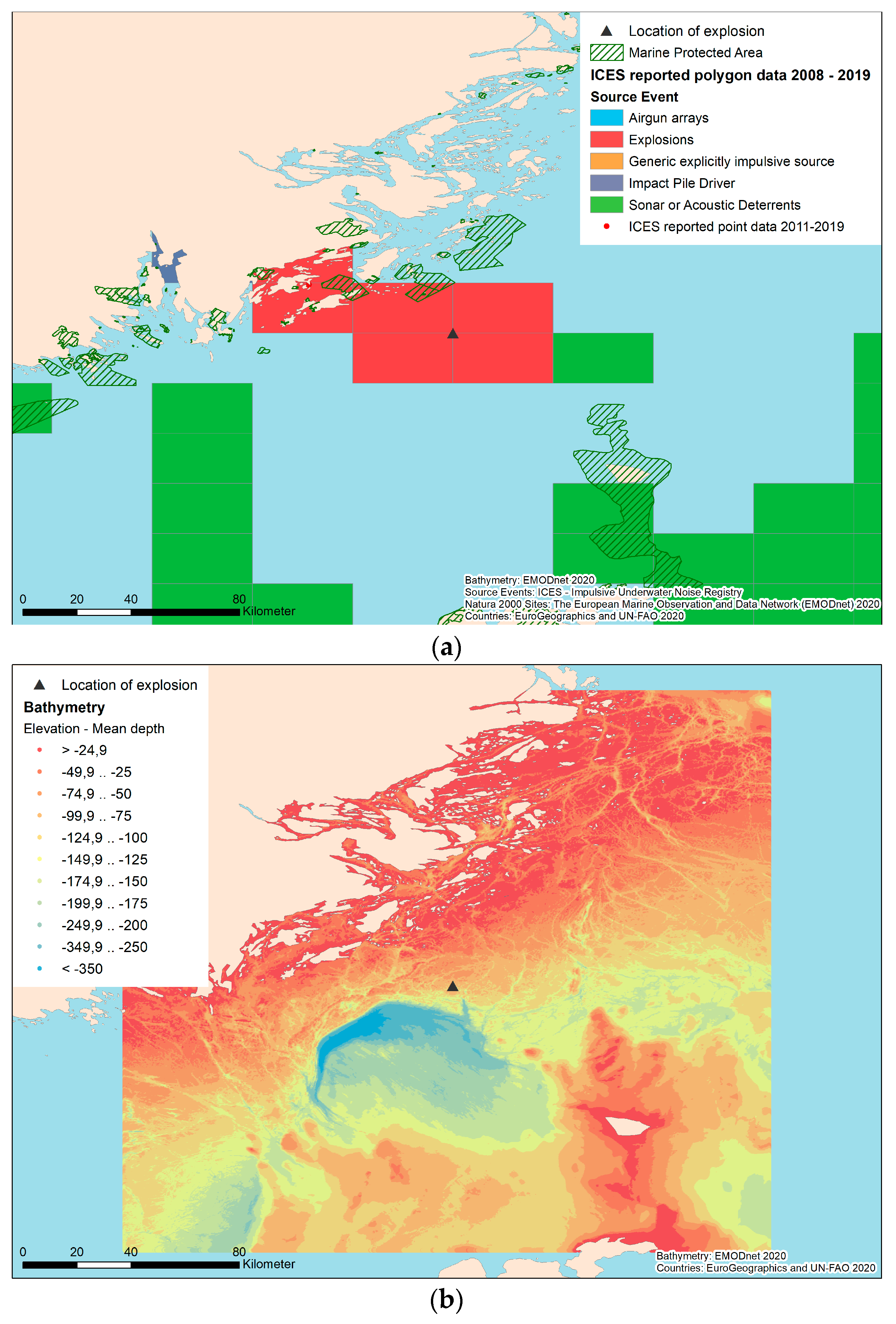
Figure 7 shows the study region including the Huvudskär MPA site and impulsive noise events reported to the noise registry.
The source locations of the explosion events were reported to the noise registry in the unit of ICES sub-rectangles only. Using this information for the assessment of affected habitat areas may therefore lead to a significant overestimation of the area affected by explosion noise when considering the entire rectangle as a potential source location. In the previous case study, we already addressed the uncertainty in estimating the affected habitat areas due to uncertainties in the reported source location. Here, we aim at the analysis of uncertainties due to different information regarding the source description. Therefore, we fixed the event location arbitrarily at the centre of the ICES rectangle as indicated by the black triangle in Figure 7.
The Natura 2000 site Huvudskär is located at a distance of approx. 16 km to the northwest of the assumed source location for this case study. Its mean water depth is −31 m (max.: −110 m, min: +0.25 m). Another relevant MPA for the protection of grey seals is Gotska Sandön-Salvorey, located at a distance of approx. 38 km to the southeast of the assumed source location with a mean water depth of −31 m (max.: −81 m, min.: +0.35 m). The water depth in the source area is approximately 85 m.
In order to determine the habitat area affected by the impulsive noise from the explosion events for a particular species, bioacoustic (threshold) criteria must be available for the calculation of the effect range associated to each source. In our test case, we arbitrarily set the bioacoustic threshold for the SEL to 164 dB re 1 µPa2s, as this value is designated as the lower limit for the reporting requirement of impulsive noise events for explosions according to TG Noise Guidance Part 3 [4]. For the estimation of the influence of the source information on the estimated effect range of the explosion noise, we compared an approach for the explosion event source description as published by the EU and an alternative source description derived from empirical observations.
In the first approach, we follow TG Noise Guidance on the description of the explosion source for the assessment of the proportion of the affected seal habitat area. Part 3 of the TG Noise Monitoring Guidance [4] considers explosions to be categorized from very low to very high, based on the “TNT equivalent charge mass” associated with an energy source level ESL. Table 6 summarizes the value code classes used for reporting to the noise registry for the source type explosions according to the explosion charge mass and the corresponding energy source level. The explosion studied in this test case has an equivalent TNT charge of 105 kg, which is assigned to the noise registry value code category “high”. Following the procedure of energy source level estimation described in the TG Noise Monitoring Guidance Part 3 [4] (formula 7 and 8 therein), this explosion charge corresponds to an energy source level of 251.2 dB re 1 µPa2m2s.
The noise registry does usually neither collect nor provide spectral information on the reported noise events. Additionally, for the explosions studied here, no information is available on this aspect. In addition to the information detailed in Table 5, Andersson [16] provides information on the frequency distribution representative for the measurements of the explosion events. For the description of the shock wave and the pressure wave, we derived an idealized estimate for the noise spectrum based on the descriptions of TNO 2014 [19] and Andersson [16]. Figure 8 shows these idealized frequency distributions used for our explosion event.
For analyzing the variation in the estimated effect ranges of explosion noise due to different choices of sound propagations formulas, we tested and compared a total of four variants, namely a shallow water propagation with the classical 15·log r law, a deep water model with 20·log r law and the empirical model (Formula (1) in comparison with results from a numerical propagation calculation by Andersson [16]). Due to the bathymetry variations, we additionally applied the cut-off frequency to all propagation models using a sound-reflecting bottom for convenience.
Figure 9 shows results for the SEL versus distance to the source location of the explosion, using the different propagation formulas and the numerical propagation calculation of the event determined by Andersson [16]. The SEL was calculated by using the determined 1 m energy source level (ESL) according to 
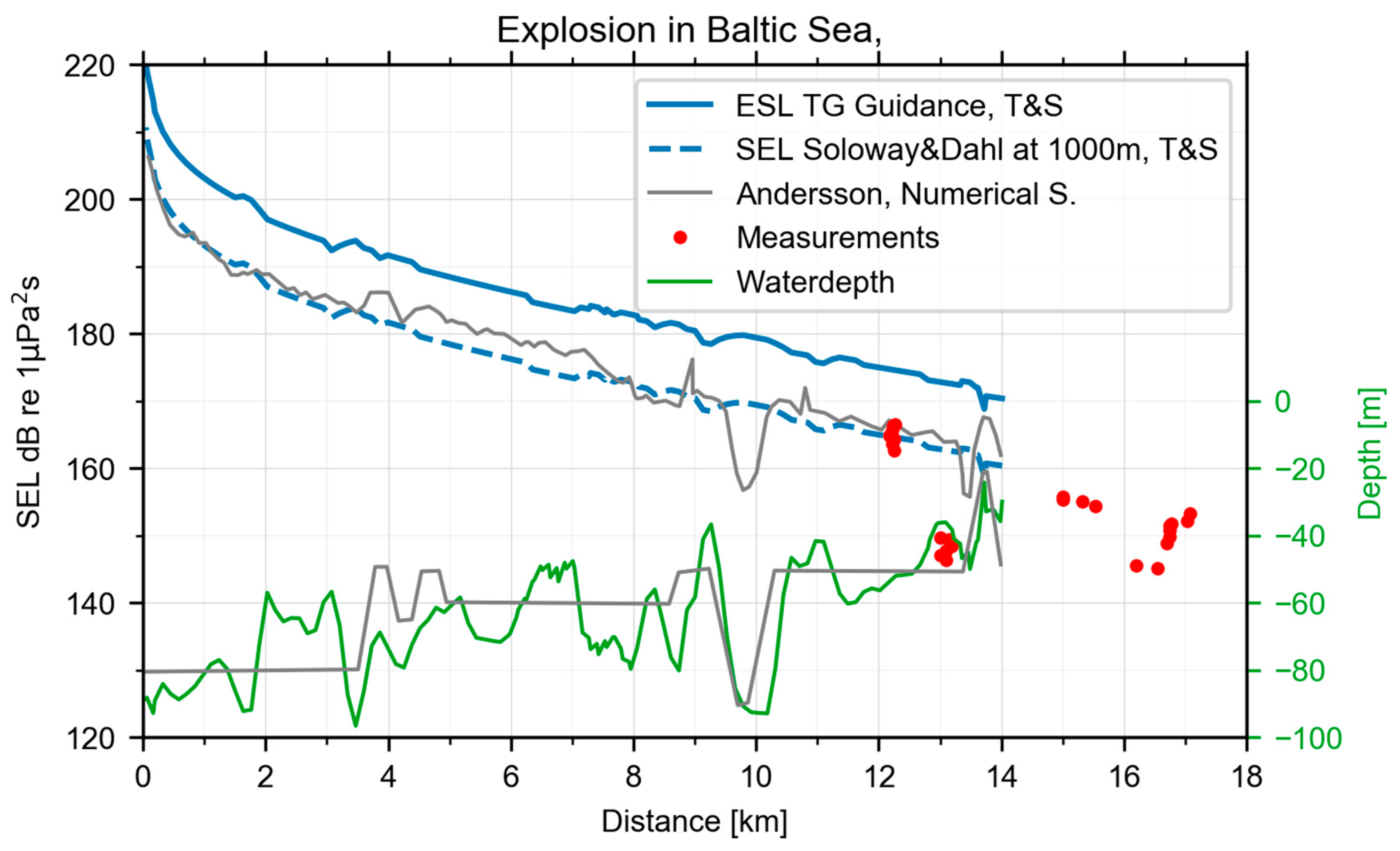
Table 6. Further, the bathymetry profiles used in this approach and used in the modelling of Andersson [16] are depicted in Figure 9. Bathymetry data used in this study (green line) was retrieved from EMODnet data and collected along the direct path from the source to measurement point. The bathymetry profiles differ in their resolution, but on average and in certain areas of strong water depth variations are in good agreement. Solid lines show results for the distance dependent SEL taking the bathymetry into account by using a corresponding cut-off frequency, while dashed lines show results without bathymetry adaptions. The different colours refer to the respective formula used to determine the results as indicated in the figure labels.
For all sound propagation formulas tested, we find an offset of at least 10 dB between the measured data and the results obtained by using the source description based on the ESL in 1 m distance to the source. These differences likely arise due to the physics of explosions, which describes near-field and far-field effects in different ways. According to these clear deviations between the calculated and measured levels according to the first approach, significant uncertainties may arise in estimated effect ranges and therewith in affected habitat areas.
In a second approach, we used an empirical formula for the description of the source strength from Soloway and Dahl [20] given by the following:
S E L = 219 + 6.14 l o g 10 W 1 3 · R W 1 3 2.12 ,
where SEL denotes the sound exposure level in dB re 1 µPa2s, R denotes the measurement range in meters and W is the charge weight in kg TNT. This formula was determined empirically by means of explosion experiments performed in shallow water of 15 m water depth, using measurement distances from 165 m to 950 m and TNT equivalent weights from 0.3 to 6.1 kg. This empirical formula was selected for the comparison here since estimated SEL values derived by this formula were reported [21] to be in good agreement with other measurements of explosions in the order of magnitude of the TNT equivalents considered here, also agreeing with well with empirical formulas derived by Cole [22].
The process of an explosion is strongly nonlinear up to a sufficient distance to the source. This distance generally depends on the explosive charge. According to Ainslie [23], non-linearities may be neglected for the physical description of the water column perturbations for distances of 5000 multiplied by the charge radius, which is given by αexp = ( 3 W / 4 π ρ e x p ) 1 / 3 with the mass density of the TNT charge of ρ e x p = 1520 kg / m 3 . This requirement is met for our explosion example. Thus, we determined the SEL of the explosion charge mass of 105 kg TNT equivalent at a reference distance of 1000 m as alternative source description. Table 7 summarizes the value code classes using Formula (2) according to the explosion charge mass and the corresponding SEL in a distance of 1000 m to the source location. According to Formula (2), we obtain an SEL of 192.9 dB re 1 µPa2s for our case study explosion.
For the analysis of the variability in effect range estimates due to the different choice for the source description, we compare the modeled results of the distance-dependent SEL from both approaches with the published measurement results. 
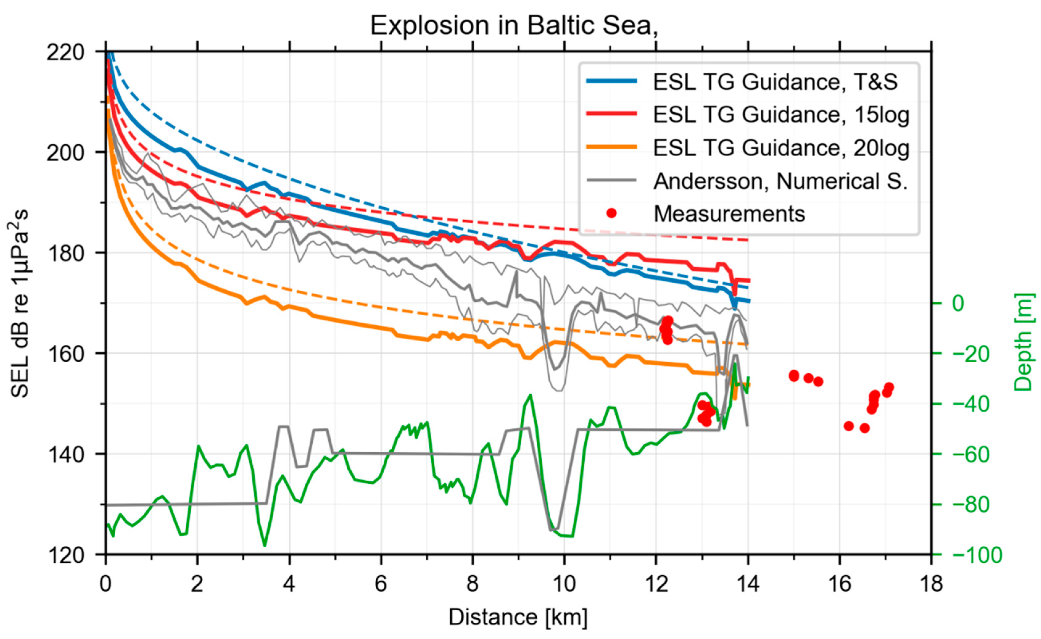
Figure 10 presents the comparison between the modeled results for the SEL versus distance to the source location from both approaches with the measurements and with the numerical calculations as published in [16] (grey curve), which were derived from an extensive study of the noise propagation using a PE model considering bathymetry and velocity profiles. Note that the near- and far-field propagation of the explosion are handled in different ways. These numerical results agree well with reported measurements (red dots) and serve as reference for the model fit obtained by using the two approaches tested in this study. The comparison shows that results of the empirical modelling and the numerical modelling achieve comparable results when using the alternative source description from the second approach using Formula (2); further, the second approach tends to reproduce the measurements better than the results obtained with the first approach.
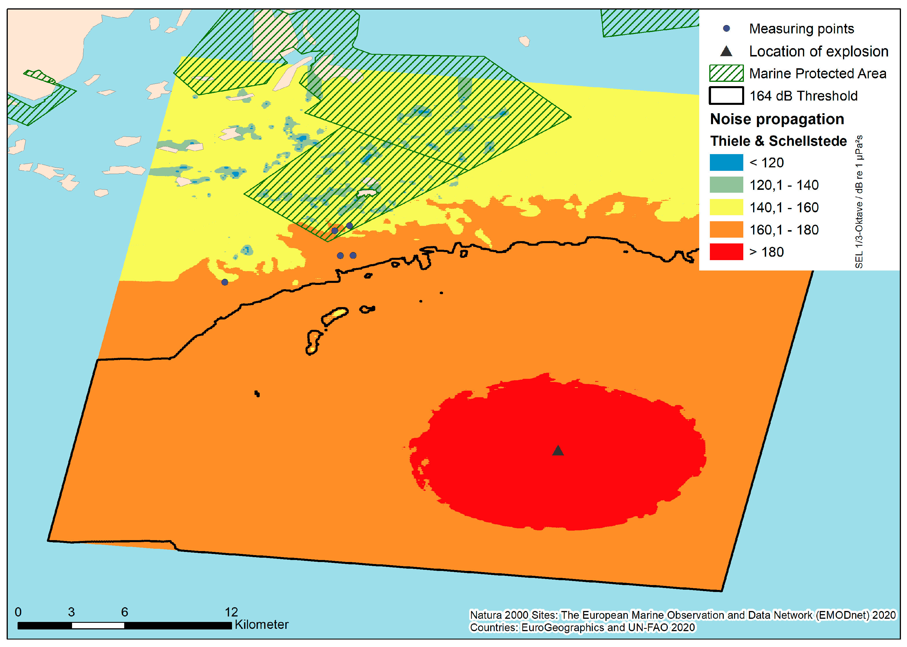
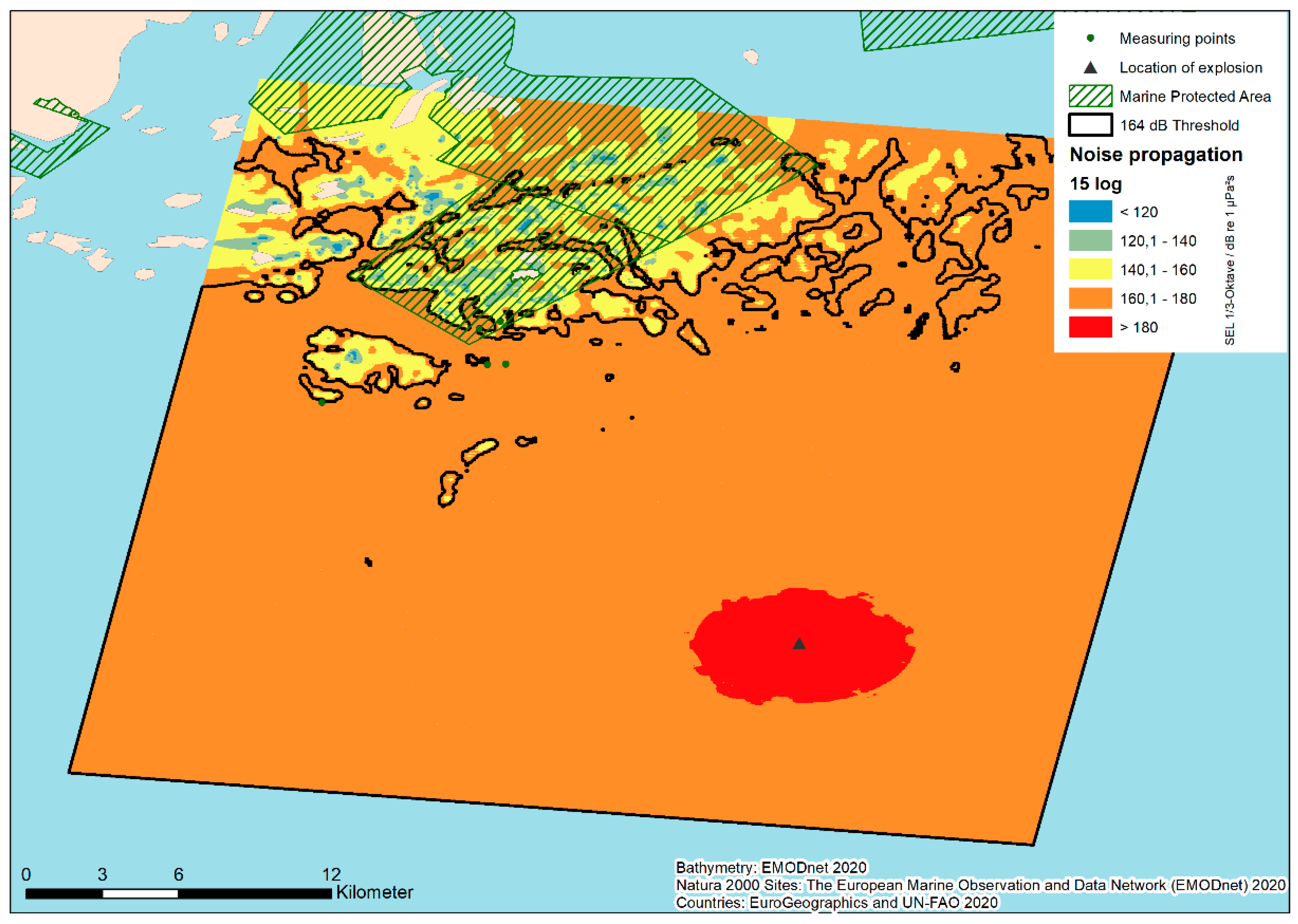
For an overview of the estimated habitat affected by the explosion noise, Figure 11 illustrates the spatial distribution of the modeled distance-dependent SEL mapped to the source area of the explosion event in the Stockholm Archipelago. For the assessment of adversely affected and unaffected habitat area, we used the bioacoustics criteria of an SEL to 164 dB re 1 µPa2s as described above. Thus, the estimated effect range of explosion noise according to the second approach for the source description and the propagation modelling with Formula (1) was found to remain outside the nearby Huvudskär Marine Protection Area (hatched). It should be noted that the use of simpler propagation models, such as 15 log r or 20 log r laws are rather imprecise for a detailed spatial assessment and pose a disadvantage for a reliable determination of the percentage of affected habitat areas, as shown in the additional map views of noise exposure levels in the Appendix B.
The first approach for the source description according to an energy source level at a distance of 1 m to the explosion source, while reasonable, has two major drawbacks. A 1 m source level is not a measurable quantity in most cases, and with the focus on far-field sound propagation, a description of the source outside the near-field yields more accurate results. In this test case, it has been demonstrated that simple propagation models accompanied by an appropriate description of the source can be used to represent the far-field sound propagation sufficiently well in comparison to published measurement results and comprehensive numerical modelling results.
For the source description, we used the empirical Formula (2) that was derived from measurements of explosion experiments. Since measurements at a certain distance provide the basis for this empirical source description approach, it would be possible to also report on measurement results of explosion noise to the regional noise registry and use these results to determine their value code category. This would have the advantage that explosions for which technical abatement measures, such as bubble curtains, were applied could be classified and reported correctly to the noise registry. Results of our study suggest that this option should be developed in a revision of the TG Noise Guidance of 2014 for the improvement of the noise registry and the assessment accuracy.
If regions in the near field of an explosion need to be considered for the protection of the marine environment, a different descriptive metric may have to be used.

3.3. Case Study: Airgun Array in the Mediterranean Sea

In our third case study, we analyze a possible handling of an assessment regarding impact on the nearby habitats of noise sensitive species when an insufficient reporting of impulsive noise events occurs. The study region for this test case is located in the Ligurian Sea of the Mediterranean Sea. The analyzed impulsive noise events took place in the year 2002. Multiple whale-watching companies noticed and reported the absence of fin whales (Balaenoptera physalus) for a period of 2 months in 2002. This absence of the species could be correlated with typical airgun array noise observed at measurement locations in the Ligurian Sea [24]. The measurements were used to derive the position of the sound source, which was determined to be near the French Îles d’Hyères outside Toulon [24]. 
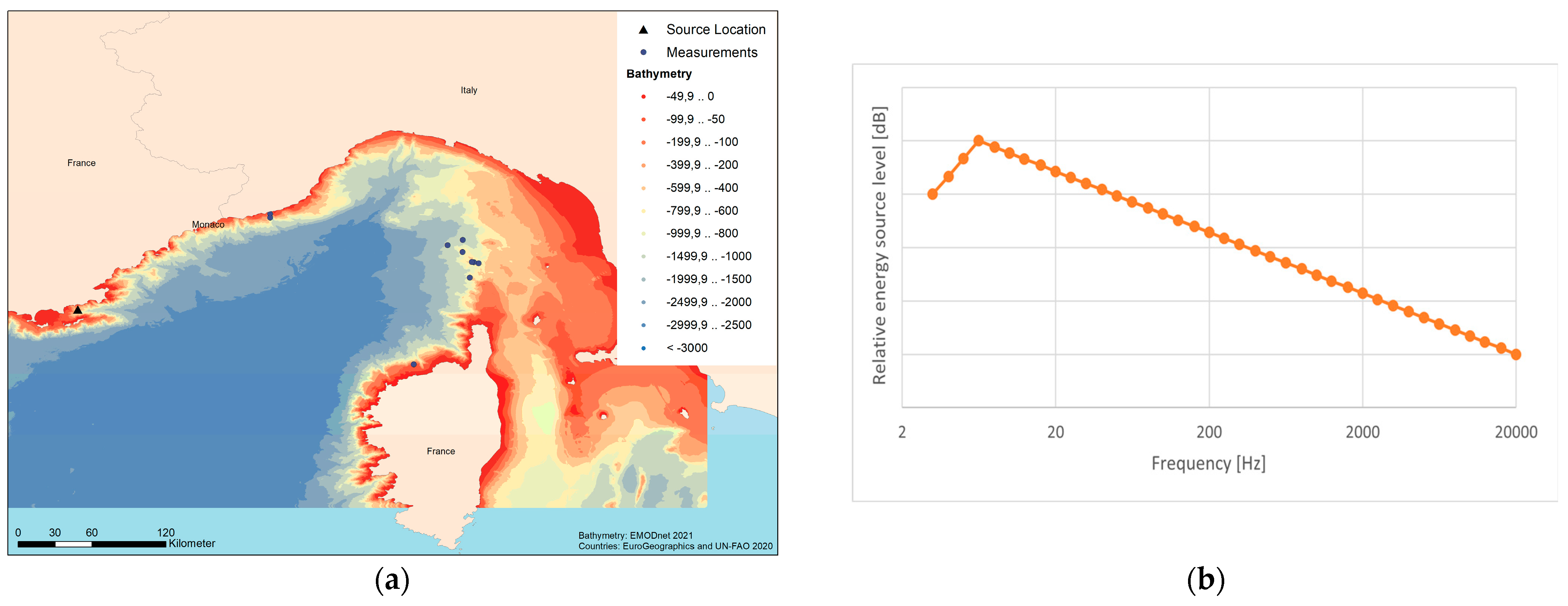
Figure 12a shows the study region for this test case and the locations of the measurement positions and the estimated source location. Since the regional noise registries under the MSFD were implemented after the year 2015, this impulsive noise activity in 2002 was not reported to any noise registry; thus, more detailed information on the activity and the source location are not publicly available. Compared to the case studies for the North Sea and the Baltic Sea, the environmental setting and the bathymetry of the study region are significantly more complex. The distance range between the events and the measurement locations is significantly higher (more than 250 km) and the water depth ranges from −80 m to −3500 m. Despite these differences in the environmental boundary conditions, the same approach as in the previous test cases was used to evaluate the test case. However, the input parameters and bioacoustic thresholds were adapted to the local conditions.
The event was defined as a point source in front of the isles of “Îles d’Hyères”. The bathymetry of the region was derived from a publicly available dataset from EMODnet [17], and is shown in the colour map in Figure 12a. A generic frequency distribution of an airgun array was used as shown in Figure 12b. For this test case, neither information on the source strength of the airgun array nor on the frequency distribution are available. Therefore, three source strengths according to [3] were considered, comprising a source level in the value code class very low (ESL of 186 dB re 1 µPa2m2s), with values according to TG Noise Guidance Part 2 [3] and, additionally, source levels in value code classes low and medium.
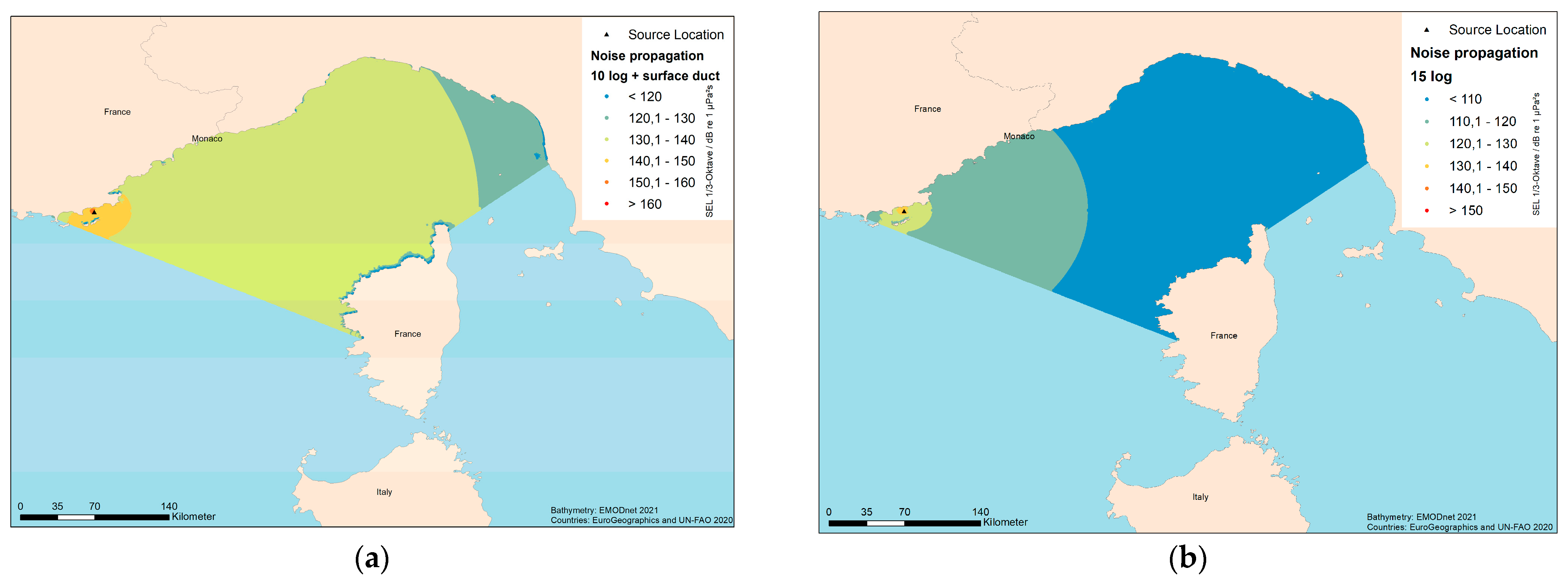
For the propagation model, four standard approaches (10 log with surface duct, 15 log r law, Formula (1) and 20 log r law) were used. In the absence of more detailed bioacoustic thresholds (frequency distribution and level values) in relation with regional cetaceans, the bioacoustic threshold was chosen here as 110 dB re 1 µPa2s to be in line with typical sound levels of ocean background noises at different frequencies, e.g., Urick [25].
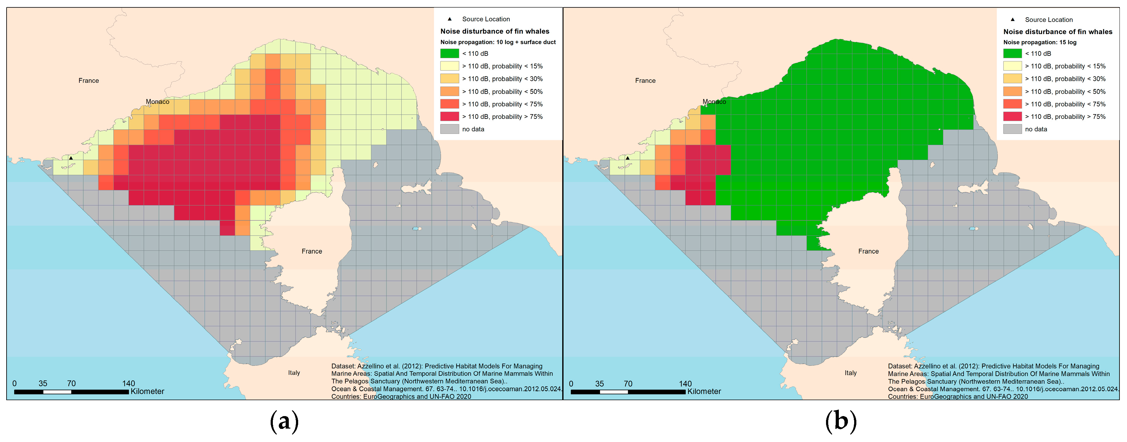
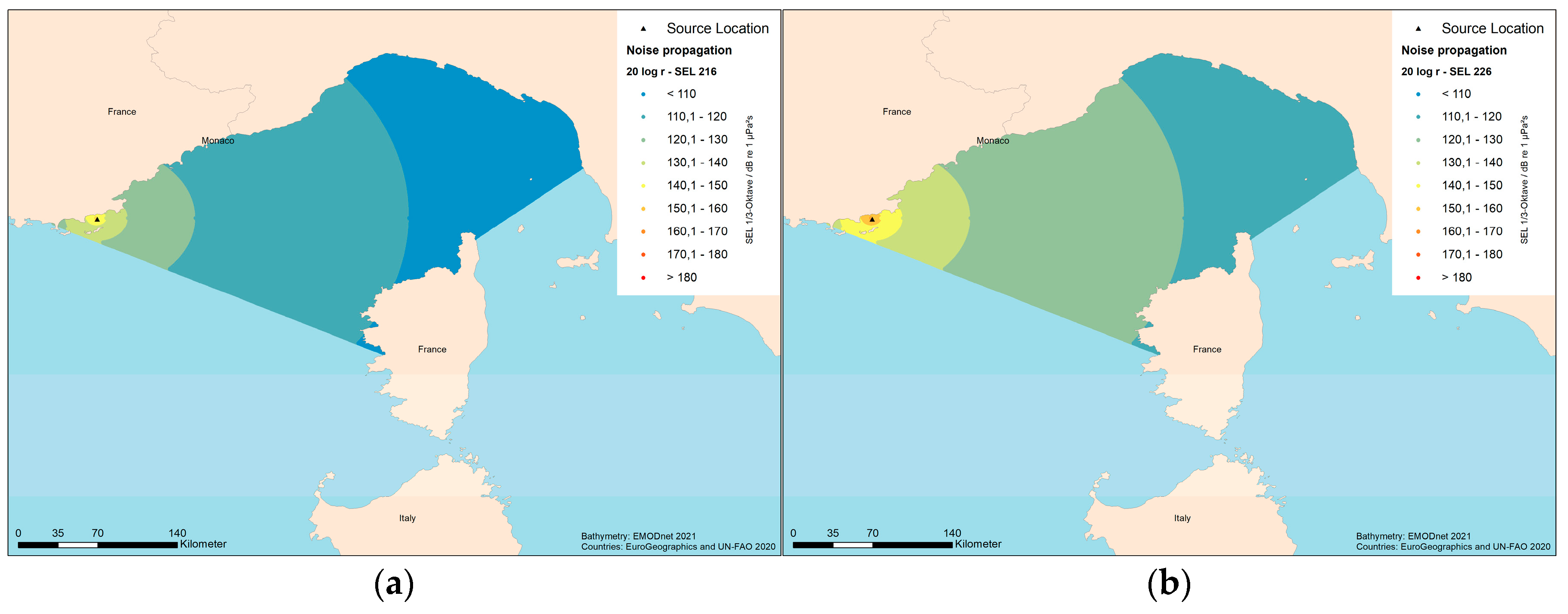
Figure 13 shows results of the analysis for the sound propagation using a 15-log attenuation law in (b), and using a 10-log attenuation law with a surface duct in (a). As expected, using the 10-log attenuation law with a surface duct yields a significantly slower decline in noise levels with propagation distance than the use of the 15-log law. Within the surface duct (or layering), the pressure loss is slower and effect ranges based on bioacoustics criteria thus extend over significantly larger distances. At the location of the observational site, the estimations of received noise levels differ by more than 60 dB, with the level using the 15-log law being close to typical background noise levels of approx. 110 dB. Further, Figure A6a,b in Appendix C shows propagation modelling results based on a ESL of 216 dB re 1 µPa2m2s and 226 dB re 1 µPa2m2s, respectively, which refer to the central value of the noise registry class ranges “low” and “medium” (cf. Table 1). These results emphasize that a solid estimation of sound propagation in the affected sea regions requires a good knowledge of regional acoustic properties in addition to a precise source description. In this case, knowledge of the depth at the source and the stratification in the water column of the sea region is essential.
To determine the impact of this noise event on the fin whale habitat, the Potentially Useable Habitat Area (PUHA) [26] was used for the assessment and a corresponding dataset of PUHA in the study area was retrieved. This PUHA dataset includes information on the probability of the occurrence of seven different marine mammal species, including fin whales. The project area was divided into grid cells of approximately 14 × 18.5 km in size. The probability of species occurrence within the habitat is influenced by abiotic factors such as water depth and seafloor slope and was augmented by sighting data [26]. According to the data, fin whales tend to stay in deeper water as shown in Figure 14. The results of the noise propagation were combined with the probability of presence for the assessment of noise disturbance of fin whales.
Figure 15 and Figure 16 show results of the propagation model combined with the PUHA dataset for the target species, fin whales, representing the probability of presence of the species in the specific area. Again, the bioacoustic criteria for a disturbance of this species was defined as being equivalent to a typical background noise level of 110 dB due to the lack of a scientifically validated bioacoustic threshold for fin whales [25]. The results for the received noise levels across the study region mapped onto the same spatial grid format of the PUHA dataset. A (spatially) averaged sound pressure level was derived for each grid cell. The probability of fin whale presence was divided into five classes: the higher the probability of a sound pressure level being above 110 dB, the higher the likely disturbance to the species. Sound pressure levels below 110 dB were classified as not disturbing for fin whales, and are shown as green-colored regions.
Figure 15 panel (a) shows results for the noise propagation using a 10-log law and a surface duct for an airgun source in the noise registry class “very low”. Results in panel (a) under the assumption of a low transmission loss due to a surface channel indicate a high likelihood that the entire habitat area of this species would be disturbed due to the slow decrease in sound pressure level. Hence, we find that by assuming an ESL of 186 dB re 1 µPa2m2s, the impulsive sound event could only be measured at the measurement locations in the Ligurian Sea (cf. Figure 12a) for a sound propagation loss according to the 10-log law with surface channel. However, based on a numeric study on the estimation of regional sound propagation for this test case performed in [27], a log 20 attenuation law was found to represent the noise propagation across the corresponding transmission path better than a lower transmission loss. Assuming an airgun source in the lowest noise registry class in combination with a transmission loss of about log 20 would thus not explain the reported absence of the fin whales in the study region.
Figure 16 shows results for the noise propagation using a 20-log law for an airgun source in the noise registry class “low” in panel (a) and “medium” in panel (b). Under the condition of an observability of the event at the measurement locations and the absence of fin whale sightings, the source strength of the airgun event would be expected to lie within the range of the noise registry class “medium”, assuming a 20-log law for the transmission loss. The analysis of PUHA here allows for a more accurate estimation of the proportions of disturbed habitat areas for a certain species due to a specific source location and source description.

4. Discussion

In this study, we analyzed the accuracy in the determination of exposed habitat areas based on data from regional noise registry using three different case studies. The common basis for these regional assessments of impulsive anthropogenic noise input and the resulting risks for biological effects is the monitoring information, which is collected annually as part of mandatory national reporting and made publicly available in the regional noise registries. Thus, the underlying data used for these assessments are open data, which make the assessment results comprehensible and reproducible. From this point of view, the MSFD monitoring concept for impulsive noise allows large-scale and recurring assessment, on the basis of which the respective achievement of environmental objectives of EU Member States can be assessed and monitored transparently. As pointed out earlier, the data framework for the assessment (including data structure, level of detail and accuracy) was defined in the form of a standardized data format, with limitations in the amount and type of information reported. Against the background of the newly established quantitative threshold values for impulsive noise under the MSFD, quantitative regional assessments will be conducted for the upcoming MSFD cycles. Based on the results of the case studies analyzed in this study the currently implemented noise registries enable the quantification of adversely affected habitats in which noise exposure has the potential to cause various types of impacts. Particularly relevant for a risk assessment for impulsive noise from sources listed in the noise registries is a cumulative assessment in conjunction with biological criteria for the risk of injury from noise input, as well as biological criteria for the risk of disturbance to marine life. The case study results confirmed that the lack of accuracy present in several parameters of the noise event data within regional noise registries has a significant influence on the quantification of exposed habitat areas. For a precise quantitative assessment, the area impacted by noise disturbances must be quantified as accurately and reliably as possible.
In our first case study, we investigated uncertainties in the estimation of impacted areas solely induced by the structure of the data basis, in particular by the allowed margin for parameters reported to the noise registry. Such uncertainties need to be addressed and delineated transparently in an assessment. The known presence of the tolerated reporting margins poses an obstacle to the clarity of the assessment results. However, the clarity of these results can be achieved by the following measures: (1) Defining binding and transparent conventions for a standardized handling of such margins would constrain the result range. (2) Increasing the proportion of precise data reporting, including voluntary additional information on the noise events, would also help achieve clarity of the results. Particularly valuable additional information concerns data on (spectral) source characteristics and their sound intensity, as well as results from in situ measurements, so long as they were collected according to standardized and well-documented methods. (3) As a relevant follow-up measure, the data basis for the next MSFD cycle could be effectively improved by an acute call for the addition of these two information aspects within the framework of the national reporting of impulsive sound data. Thus, it is recommended to improve and complete the quality of the input data by reporting higher resolution data (e.g., exact positions of an event, information on the application and resulting noise abatement of technical reduction measures) to the noise registries. Furthermore, it is recommended to provide standardized frequency spectra via the noise registries to be used for the assessments of respective sound events. Such a standardized approach to characterize the sources would contribute to comparability in the determination of exposed areas.
In our second case study, we focused on the examination of different input data to describe the sound source and its impact on the results for estimating noise exposure. The results show that the best possible source information, especially for far-reaching intense impulsive noise sources, is crucial for a quantitative assessment and that improving the source information (e.g., standardized frequency spectra, in situ measurement results) increases the reliability in the impacted habitat areas. The impulsive sound input from explosions holds a special significance within the set of reported noise activities in the noise registry. The focus on disturbance of marine life, set for the other activities, does not suffice for explosions. On the one hand, the intensity of this activity is particularly high compared to the other impulsive sound generating human activities considered and, in particular, carries the risk of injury to marine life in a wider area around the source. On the other hand, the single explosion event itself is a transient event that has no significant temporal extent compared to other sound generating activities. Moreover, in the case of explosion, a physical distinction must be made between the near field with nonlinear pressure disturbance and the far field with linear acoustic sound propagation. Due to the special characteristics mentioned above, explosions may need a separate consideration in future assessments, e.g., for the evaluation of effects close to the source. In order to effectively improve the data basis for the next MSFD cycle, our case study shows the potential to use further empirical formulas for the description of the source strength, especially those that could be further verified and optimized by measurements for different regional sea areas in the future. In connection with this, it is advisable that measurement results from in situ measurements of the far-field sound input from explosions are reported to the regional noise registries and published for all marine regions. The application of the empirical formulas does not represent a considerable additional effort, so that the application seems suitable for a regional assessment. As with the first case study on pile driving, there is a significant need to include the use of noise abatement methods in the reporting and to provide a source description for explosions. Effect ranges can be reduced significantly by technical measures. The neglect of such measures in the source description represents one of the most significant inaccuracies in the assessment with respect to intense events. In order to adequately reflect the effect of measures in the assessment, immediate action should be taken to include them in the reporting concept.
In our third case study, we considered an impulsive noise source event that was not recorded in the noise registry and estimated associated effect ranges and their overlap with nearby habitats of noise sensitive species. Despite considerable uncertainties in source strength and associated effect ranges, an estimation for the possible habitat area impacted was enabled by a risk analysis based on the limited knowledge on the presence of a certain type of impulsive sound source and the knowledge of existing habitats. In the future, further gaps in the reporting of noise events have to be expected, both in terms of the completeness of occurred events and in terms of the description of the sources. For the purpose of achieving assessments that are as accurate and comprehensive as possible despite these caveats, we may extend our common data basis with a sufficient number of detailed observations (e.g., far-field in situ measurements), serving the validation of assumptions on source properties and effect ranges for all regions and sub-regions.
In conclusion, (a) the present information in the registries was found to be suitable to be used to estimate impact on habitats, (b) the data completeness of the registries must be improved, (c) the separation of sources as proposed by the EU TG Noise (Table 2) suggests that different biological threshold criteria have to be set for different sources and (d) the test cases showed that it is possible to use simple propagation models to estimate first-order effect ranges in shallow seas and deep oceans. The most important priorities for further improvement of the input data assembled in regional noise registries based on the results of the case studies analyzed here are as follows:
The increase in the reporting of events with higher resolution (e.g., exact geographic positions of an event instead of polygon based information);
The increase in the reporting details regarding the application of mitigation and abatement measures;
The integration of standardized frequency spectra for the description of the noise sources with the aim of achieving comparability when determining exposed habitats.
It is further recommended to use standardized procedures, at least within the respective regional seas, to be able to produce comparable assessment results between habitats and reproducible assessment results between different years. The most important aspects for the standardization are as follows:
The further standardization of noise propagation calculations in combination with biological threshold levels, or the consideration of predefined effect range buffers;
The standardization of the usage of noise registry information for the source level estimation (e.g., using a precautionary estimate of source levels by considering the upper boundary of the value code classes as worst-case approximation of source levels) or the improvement of source level information in the registry.

Author Contributions

Conceptualization, C.J., J.F.B. and P.S.; Methodology, A.M.; Software, R.E.; Validation, A.M., J.F.B. and P.S.; Formal analysis, A.M. and R.E.; Writing—original draft, C.J., A.M.; Writing—review & editing, A.M., J.F.B. and P.S.; Visualization, R.E.; Supervision, J.F.B. and P.S.; Project administration, C.J.; Funding acquisition, C.J., J.F.B. and P.S. All authors have read and agreed to the published version of the manuscript.

Funding

This research was funded by the EU Directorate-General of the Environment under the MSFD 2020 Call, Grant Agreement No.110661/2020/839605/SUB/ENV.C.2.

Institutional Review Board Statement

Not applicable.

Informed Consent Statement

Not applicable.

Data Availability Statement

Datasets used in this analysis and reports from the HARMONIZE project are available at https://www.ices.dk/data/data-portals/Pages/impulsive-noise.aspx, https://www.emodnet-bathymetry.eu/data-products, https://www.eea.europa.eu/ds_resolveuid/DAT-68-en and https://www.bsh.de/DE/THEMEN/Forschung_und_Entwicklung/Aktuelle-Projekte/Harmonize/Harmonize_node.html, accessed on 8 December 2021. All other data and information used by the authors of this study are available upon request.

Acknowledgments

The analyses presented here were performed within the context of the EU project HARMONIZE, which was funded under the MSFD 2020 Call (Grant Agreement No. 110661/2020/839605/SUB/ENV.C.2) for the purpose of supporting the implementation of the MSFD by contributing to a harmonized quantitative assessment of impulsive underwater noise, which can be implemented immediately for the next MSDF reporting cycle in all regions and sub-regions and which is directly compatible with the newly developed quantitative EU threshold values. The authors would like to thank all HARMONIZE project team members and the associated research project team members for their indispensable support, expertise and enthusiasm throughout the project. Special thanks go to Ben Schmidt, Benedikt Niesterok, Isabella Kratzer, Maria Boethling, Thierry Maquil and Wiebke Hahne. Further thanks go to all members and participants of EU TG Noise meetings, contributing to fruitful discussions on the content of this study. The authors would like to thank the anonymous reviewers for valuable comments that helped to improve this manuscript.

Conflicts of Interest

The authors declare no conflict of interest. The funders had no role in the design of the study; in the collection, analyses, or interpretation of data; in the writing of the manuscript; or in the decision to publish the results.

Appendix A

Figure A1. (a) Value code per year within ICES polygons dataset; (b) Value code per year within ICES points dataset.
Jmse 11 00847 g0a1
Figure A2. (a) Value code per year within INR-MED polygons dataset; (b) Value code per year within INR-MED points dataset.
Jmse 11 00847 g0a2
Figure A3. Value code per year within EMODnet polygons dataset.
Jmse 11 00847 g0a3

Appendix B

Figure A4. Sound exposure level map using 20 log law with consideration of the bathymetry.
Jmse 11 00847 g0a4
Figure A5. Sound exposure level map using 15 log law with consideration of the bathymetry.
Jmse 11 00847 g0a5

Appendix C

Figure A6. Pressure map due to an airgun array in the Mediterranean Sea, using (a) 20 log with ESL = 216 dB re 1 µPa2m2s and (b) 20 log law with ESL = 226 dB re 1 µPa2m2s.
Jmse 11 00847 g0a6

References

  1. Commission Decision (EU) 2017/848 of 17 May 2017 Laying down Criteria and Methodological Standards on Good Envi-ronmental Status of Marine Waters and Specifications and Standardised Methods for Monitoring and Assessment and Re-pealing Decision 2010/477/EU. Official Journal of the European Union, L125/43, Document 32017D0848. Available online: https://mcc.jrc.ec.europa.eu/documents/ComDec/Com_dec_GES_2017_848_EU.pdf (accessed on 1 April 2023).
  2. Dekeling, R.P.A.; Tasker, M.L.; Van der Graaf, A.J.; Ainslie, M.A.; Andersson, M.H.; André, M.; Borsani, J.F.; Brensing, K.; Castellote, M.; Cronin, D.; et al. Monitoring Guidance for Underwater Noise in European Seas, Part I: Executive Summary, Luxembourg, Publications Office of the European Union. JRC Sci. Policy Rep. EUR 2014, 138. [Google Scholar] [CrossRef]
  3. Dekeling, R.; Tasker, M.; Van Der Graaf, S.; Ainslie, M.; Andersson, M.; André, M.; Borsani, J.; Brensing, K.; Castellote, M.; Cronin, D.; et al. Monitoring Guidance for Underwater Noise in European Seas—Part II: Monitoring Guidance Specifications; EUR 26555; Dekeling, R., Tasker, M., Ferreira, M., Zampoukas, N., Eds.; Publications Office of the European Union: Luxembourg, 2014; ISBN 978-92-79-36339-9. JRC88045. [Google Scholar] [CrossRef]
  4. Dekeling, R.; Tasker, M.; Van Der Graaf, S.; Ainslie, M.; Andersson, M.; André, M.; Borsani, J.; Brensing, K.; Castellote, M.; Cronin, D.; et al. Monitoring Guidance for Underwater Noise in European Seas—Part III: Background Information and Annexes; EUR 26556; Dekeling, R., Tasker, M., Ferreira, M., Zampoukas, N., Eds.; Publications Office of the European Union: Luxembourg, 2014; ISBN 978-92-79-36340-5. JRC88885. [Google Scholar] [CrossRef]
  5. International Council for the Exploration of the Sea (ICES): Impulsive Underwater Noise. Available online: https://www.ices.dk/data/data-portals/Pages/impulsive-noise.aspx (accessed on 8 December 2021).
  6. Enguix, I.F.; Sánchez Egea, M.; Molina, P.R.; Maglio, A.; Salvias, M. The International Impulsive Noise Register for the Mediterranean Sea Region (INR-MED). In Proceedings of the OCEANS, Marseille, France, 17–20 June 2019; pp. 1–3. [Google Scholar] [CrossRef]
  7. EMODnet. Impulsive Noise Events Registry. Available online: https://catalogue.emodnet-physics.eu/geonetwork/srv/api/records/bccf1db2d12372852b1c28207bdc771ed275014a (accessed on 8 December 2021).
  8. Müller, A.; Juretzek, C.; Borsani, J.F.; Sigray, P.; Eigenmann, R.; Niesterok, B. Threshold Value Concept—Assessment Framework for Impulsive Noise for Immediate Application in All EU Regions—Part II: Technical Aspects. Funded by DG Environment, Grant Agreement No. 110661/2020/839605/SUB/ENV.C.2; European Commission: Luxembourg, 2022. [Google Scholar]
  9. Müller, A.; Juretzek, C.; Borsani, J.F.; Sigray, P.; Eigenmann, R.; Niesterok, B. Threshold Value Concept—Assessment Framework for Impulsive Noise for Immediate Application in all EU Regions—Part III: Background Information, Technical Details and Recommendations. Funded by DG Environment, Grant Agreement No. 110661/2020/839605/SUB/ENV.C.2; European Commission: Luxembourg, 2022. [Google Scholar]
  10. ISO 18405:2017; Underwater Acoustics—Terminology. ISO: New York, NY, USA, 2017.
  11. Müller, A.; Maquil, T.; Eigenmann, R.; Juretzek, C. Classification and Assessment of Impulsive Noise with and without Mitigation Measures Exposure Index Based on a Habitat Approach. Technical Report, R&D “Assessment Approaches for Underwater sound Monitoring Associated with Offshore Approval Procedures, Maritime Spatial Planning and the Marine Strategy Framework Directive—BeMo”, Ordner Nr. 10036955, Bundesamt für Seeschifffahrt und Hydrographie (BSH). 2020. Available online: https://www.bsh.de/DE/PUBLIKATIONEN/_Anlagen/Downloads/Projekte/BeMo-Indicators_Habitat-Approach.pdf (accessed on 29 May 2020).
  12. Ainslie, M.A.; Leaper, R.; Merchant, N.; Norro, A.; Müller, A. 15th TG Noise Meeting: Revision of the “TG Noise Monitoring Guidance“ Part 1: Source Levels of Pile-Driving Noise with/without Noise Protection Measures Update, TG Noise Meeting, 2 June 2020. Available online: https://circabc.europa.eu/ui/group/326ae5ac-0419-4167-83ca-e3c210534a69/library/6905c8da-0b72-41c6-9f15-17a0cbf07e96/details (accessed on 5 June 2020).
  13. ISO 18406:2017; Underwater Acoustics—Measurement of Radiated Underwater Sound from Percussive Pile Driving. ISO: New York, NY, USA, 2017.
  14. Thiele, R.; Schellstede, G. Standardwerte zur Ausbreitungsdämpfung in der Nordsee, Forschungsanstalt der Bundeswehr für Wasserschall und Geophysik; FWG-Bericht 1980-7; Bundeswehr: Bonn, Germany, 1980. [Google Scholar]
  15. Merchant, N.D.; Faulkner, R.; Martinez, R. Marine Noise Budgets in Practice. Conserv. Lett. 2017, 11, e12420. [Google Scholar] [CrossRef]
  16. Andersson, M.H.; Nöjd, A.; Carlström, J. Kunskapsunderlag om Undervattensexplosioner och Marina Djur; Teknisk Rapport FOI-R--4413—SE; Totalförsvarets forskningsinstitut FOI: Stockholm, Sweden, 2017. [Google Scholar]
  17. EMODnet. Bathymetry, Understanding the Topography of the European Seas. Available online: https://www.emodnet-bathymetry.eu/data-products (accessed on 30 June 2021).
  18. European Environment Agency. Natura 2000 Data—The European Network of Protected Sites. Available online: https://www.eea.europa.eu/ds_resolveuid/DAT-68-en (accessed on 4 May 2021).
  19. TNO. Assessment of Impact of Underwater Clearance of Historical Explosives by the Royal Netherlands Navy on Harbour Porpoises in the North Sea; TNO R10916; TNO: The Hague, The Netherlands, 2014. [Google Scholar]
  20. Soloway, A.G.; Dahl, P.H. Peak sound pressure and sound exposure level from underwater explosions in shallow water. J. Acoust. Soc. Am. 2014, 136, EL219–EL223. [Google Scholar] [CrossRef] [PubMed]
  21. Salomons, E.M.; Binnerts, B.; Betke, K.; von Benda-Beckmann, A.M. Noise of underwater explosions in the North Sea. A comparison of experimental data and model predictions. J. Acoust. Soc. Am. 2021, 149, 1878–1888. [Google Scholar] [CrossRef] [PubMed]
  22. Cole, R.H. Underwater Explosions; Princeton University Press: Pricton, NJ, USA, 1948. [Google Scholar]
  23. Ainslie, M.A. Principles of Sonar Performance Modeling; Springer: Berlin/Heidelberg, Germany, 2010. [Google Scholar]
  24. Borsani, J.F.; Clark, C.W.; Nani, B.; Scarpiniti, M. Fin whales avoid loud rhythmic low-frequency sounds in the Ligurean Sea. Bioacoustics 2008, 17, 161–163. [Google Scholar] [CrossRef]
  25. Urick, R.J. Principles of Underwater Sound, 3rd ed.; McGraw-Hill: New York, NY, USA, 1983. [Google Scholar]
  26. Azzellino, A.; Panigada, S.; Lanfredi, C.; Zanardelli, M.; Airoldi, S.; di Sciara, G.N. Predictive Habitat Models For Managing Marine Areas: Spatial And Temporal Distribution Of Marine Mammals Within The Pelagos Sanctuary (Northwestern Mediterranean Sea). Ocean. Coast. Manag. 2012, 67, 63–74. [Google Scholar] [CrossRef]
  27. Hemon, E.; Clorennec, D.; Folegot, T. Harmonize EU Project, D11C1—Underwater Sound Modelling Test Cases; Technical Report Number QO.20210924.01.RAP.001.01A; Quiet-Oceans: Brest, France, 2022. [Google Scholar]
Figure 1. Completeness of available data regarding the parameter source event type (blue) and values code type (orange) as percentage of present/missing entries, provided for the different regional datasets.
Jmse 11 00847 g001
Figure 2. Influence on the propagation range of noise levels to fall below certain thresholds (SEL 140 dB re 1µPa2s), based on the source intensity difference implied due to the value code classification. The transmission loss was calculated with Formula (1).
Jmse 11 00847 g002
Figure 3. Propagation radius range of exceedance of an SEL of 140 dB re 1 µPa2s for different value code classes (pile driving). The transmission loss was calculated with Formula (1).
Jmse 11 00847 g003
Figure 4. Exposed area (MPA Southern North Sea) of interest depending on value code class.
Jmse 11 00847 g004
Figure 5. Possible positions of a source within a rectangle as input assumption for an assessment.
Jmse 11 00847 g005
Figure 6. Change of exposed area depending on position description: ((yellow) complete rectangle, (green) lower left corner, (blue) centroid, (red) upper right corner).
Jmse 11 00847 g006
Figure 7. (a) Map of the study region including the Huvudskär Natura 2000 site (hatched area), the explosion events reported to the noise registry (red rectangles) and the explosion location as selected for this study (black triangle); (b) bathymetry in the vicinity of the explosion location selected for this study (black triangle).
Jmse 11 00847 g007
Figure 8. Idealistic frequency distributions assumed for the description of the shock wave and the pressure wave of an explosion event.
Jmse 11 00847 g008
Figure 9. Modelled SEL versus distance to the explosion source location in the direction of measurement locations taking the bathymetry (via the cut-off frequency) into account (solid lines) and neglecting bathymetry (dashed lines). The different colours refer to the propagation formula used to determine the SEL according to the labels. The water depth used in this study from georeferenced data used to calculate the cut-off frequency for the propagation estimates illustrated by the solid lines is shown in green. Results of numerical calculations presented with data from Andersson [16] including the water depth are shown in grey, where the thin grey lines depict the spread of the transmission loss predictions.
Jmse 11 00847 g009
Figure 10. Comparison of modelled SEL over distance from both approaches with measurement results and with numerical results as published in [16]. For both approaches, the same Formula (1) and bathymetry was used for the noise propagation modelling. The blue solid line shows the result obtained by using the first approach for the source description according to TG Noise Guidance Part 3. The blue dashed line shows the result obtained by using the second approach according to Formula (2). Results of the numerical calculations with data from Andersson’s [14] including the bathymetry used are shown in grey.
Jmse 11 00847 g010
Figure 11. Sound exposure level map using Formula (1) with consideration of the bathymetry and source description according to Formula (2).
Jmse 11 00847 g011
Figure 12. (a) Bathymetry in the study area between source (black triangle) and measurement locations in the Ligurian Sea (blue dots). (b) Idealistic frequency distribution used for the source description of the airgun array.
Jmse 11 00847 g012
Figure 13. Pressure map due to an airgun array in the Mediterranean Sea using a 10-log law with a surface duct in (a) and using a 15-log law in (b).
Jmse 11 00847 g013
Figure 14. Probability of fin whale presence using data for potentially usable habitat areas as published in [26].
Jmse 11 00847 g014
Figure 15. Potentially usable habitat probability for cetaceans exposed due to an airgun array (ESL = 186 dB re 1 µPa2m2s) event, with an exposure threshold 110 dB in using a 15-log law in (b), and a 10 log with a surface duct in (a).
Jmse 11 00847 g015
Figure 16. Potentially usable habitat probability for cetaceans exposed due to an airgun array event with an exposure threshold 110 dB, using a 20-log law (a) with ESL= 216 dB re 1 µPa2m2s and (b) with ESL = 226 dB re 1 µPa2m2s.
Jmse 11 00847 g016
Table 1. Categorization of specific source levels (energy source level ESL (dB) re 1 µPa2m2s (single events) and source level re 1 µPa2m2) into classes proposed by TG Noise with data from [3]. Source levels were retrieved from received levels of sound exposure level (SEL) and sound pressure level (SPL) at a distance of 1000 m, with a propagation loss of 46 dB (shallow water).
Value Code CategoryESL [dB]
re 1 µPa2m2s
Multiple
Impulsive Source
ESL re 1 µPa2m2s
Single
Impulsive Source
SL dB re 1 µPa2m2
Non-Pulse/Continuous Sounds
Very low186–210210–234176–200
Low211–220235–244201–210
Medium221–230245–254211–220
High230255–264221
Very high 265
Table 2. Categorization of specific source levels and associated physical quantities into classes as proposed by TG Noise with data from [2].
Value Code CategoryESL [dB] re 1 µPa2m2s
Generic Explicitly Impulsive Source
SL [dB] re 1 µPa2m2
Sonar or Acoustic Deterrents
SLzp [dB] re 1 µPa2m2
Airgun Arrays (Zero to Peak Source Level)
Explosions [eq. TNT Charge Mass kg]Pile Driving [Hammer Energy MJ]
Very low186–210176–200209–2330.008–0.210−0.28
Low211–220201–210234–2430.220–2.10.29–2.80
Medium221–230211–220244–2532.11–212.81–28
High23022025322 –21028
Very high 210
Table 3. Revised categorization of specific source levels for pile driving events into classes as proposed by TG Noise as adapted from [11], with permission from Müller et al., 2020.
Value Code CategoryPile Driving [kJ]Classes
(Revised)
SEL (750 m)
dB re 1 µPa2s
Lp,pk (750 m)
dB re 1 µPa2s
Very low0.25–28A141–161163–183
Low29–280B162–171184–193
Medium290–2800C172–181194–203
High 2900–28,000D182–191204–213
Very high29,000–E192–214–
Table 4. Percentage of exposed area (MPA Southern North Sea) of interest as shown in Figure 4 and depending on value code category.
Value Code CategoryExposed Area
Very low0%
Low0.84%
Medium6.65%
High 18.69%
Very high-
Table 5. Selection of reported measurement results with data from [16].
Explosion Depth
m
SPL
dB re 1 µPa
SEL
dB re 1 µPa2s
Distance
km
30 m188.6162.412.2
50 m177.1154.415.2
Unknown167.3146.616.4
30 m168.8149.513.1
20 m172.7150.316.8
Table 6. Source description according to TG Noise Guidance for the classification of explosion noise with data from [4].
Value Code CategoryEq. TNT Charge Mass kgESL
dB re 1 µPa2m2s
Very low0.008 kg210.0
0.210 kg224.2
Low0.220 kg224.4
2.10 kg234.2
Medium2.11 kg234.2
21 kg244.2
High22 kg244.4
210 kg254.2
Very highabove 210 kg254.2
Test case105 kg251.2
Table 7. Source description according to Formula (2) obtained for a distance of 1000 m to the source for the classification of explosion noise.
Value Code CategoryTNT Mass g/kgSEL (1000 m)
dB re 1 µPa2s
Very low8 g166.6
210 g175.6
Low220 g175.8
2.10 kg182
Medium2.11 kg182
21 kg188.4
High22 kg188.5
210 kg194.8
Very highabove 210 kg194.8
Test case105 kg192.9
Disclaimer/Publisher’s Note: The statements, opinions and data contained in all publications are solely those of the individual author(s) and contributor(s) and not of MDPI and/or the editor(s). MDPI and/or the editor(s) disclaim responsibility for any injury to people or property resulting from any ideas, methods, instructions or products referred to in the content.

