Abstract
To study the influence of launch conditions and wave interference on the stability of submersible aerial vehicles at the water–air interface, a coupling model for water-exit motion of submersible aerial vehicles was established by using the RNG k-ε turbulence model and VOF method. The water-exit processes of submersible aerial vehicles under different initial inclination angles and velocities were numerically simulated and the effects of initial inclination angle and velocity on the water-exit motion of submersible aerial vehicles were obtained. Based on the response surface function theory, a mathematical model for the motion stability of submersible aerial vehicles at the water–air interface was established, so that the submersible aerial vehicle’s pitch angle and velocity at the end of vehicle’s water-exit process, corresponding to any initial inclination angle and velocity, can be solved. The deviation between the simulated calculation result and the established fitting function model result was 2.7%. The minimum water-exit velocity of submarine aerial vehicles should be greater than 10.8 m/s. The research provides technical support for the trans-media motion stability analysis and hydrodynamic performance design of the submersible aerial vehicle.
1. Introduction
Submersible aerial vehicles have the advantages of concealment, mobility and strong offensive ability and they have received increasing attention. The water-exit process is the key to the successful launch of submersible aerial vehicles and it involves two-phase interfaces. The missile body is affected by marine environment factors such as ocean currents, waves and so on, and there are great differences in pressure, density, viscosity and other fluid characteristics between water and air [1], which makes the force on the submersible aerial vehicle change greatly when it crosses the interface between water and air [2]. Therefore, the mechanical environment of the submersible aerial vehicle water-exit process is very complex. Furthermore, the process of flying out of the water surface is also affected by waves, which increase the randomness of the water-exit process [3]. The keys to trans-media motion are the water-entry (or -exit) angle and velocity [4]. The process of a submarine-launched missile flying out of water is strongly interfered with by the wind and waves in the ocean. During the water-exit process of a submarine aerial vehicle, the surface of the submarine aerial vehicle is subjected to the impact of water and fluid elastic forces. However, the surface material of the submarine aerial vehicle has sufficient strength, so it can resist the impact of water [5]. If the submersible aerial vehicle does not have an appropriate water-exit angle and velocity, the initial conditions of flight will not be reached after it rushes out of the water surface [6], so that the vehicle will not enter the correct trajectory.
As for the water-exit movement of the bodies with different shapes, some related research has been conducted by previous researchers. Cao [7] used the method of numerical simulation to study the trajectory of submersible aerial vehicle motion in the water after vertical launch, calculated the flow field of the vehicle in the process of water-exit and analyzed the impact of the change of flow field pressure on the vehicle trajectory, but did not analyze the influence of different launch factors on the vehicle’s water-exit trajectory. Wang [8] built the model of three-dimensional water-exit trajectory of submersible aerial vehicles based on dynamic mesh technique but only simulated the water-exit motion process of submarine-launched missiles under a specific launch condition. They obtained the characteristics of underwater trajectory and attitude angle of the submarine-launched missile but could not discern the influence of different launch conditions on the stability of the submarine-launched missile’s water-exit motion. Hu [9] established the hydrodynamic model of Morphing Unmanned Submersible Aerial Vehicle (MUSAV) exiting the water surface obliquely and analyzed the water-to-air process of the vehicle but lacked the prediction analysis of the vehicle’s trans-medium motion stability. Yuan [10] established the water-exit trajectory model of unpowered submersible aerial vehicle carriers and carried out relevant experiments, providing support for simulation and analysis of the submersible aerial vehicle’s water-exit trajectory, but did not carry out research on the influence of pitch angle and velocity on the water-exit movement of submarine aerial vehicles. Siddall [11] proposed and designed a new amphibious aircraft (AquaMAV); this work emphasized the concept of bionic design and demonstrated the feasibility of the waterjet propulsion to fly out of the water but did not analyze the hydrodynamic performance of the amphibious aircraft’s water-exit process. Moshari [12] established a dynamic mesh model to solve water-exit of a circular cylinder based on Volume of Fluid (VOF) method and finite volume discretization-based code but did not analyze the variation of attitude angle and other motion characteristics of the cylinder during the cylinder’s water-exit process. Chu [13] simulated the water-exit process of a cylindrical body and captured the interaction of free surface during the water-exit process; the velocity and acceleration of the cylinder were also analyzed but they did not analyze the influence of launch conditions such as inclination angle and velocity on the trans-medium motion of the cylinder. Ni and Wu [14] researched the vertical water-exit process of a buoyant spheroid by combining boundary element method (BEM) with slender body theory (SBT) but did not comprehensively analyze the slender body’s water-exit movement performance under different launch conditions. Xiao et al. [15] studied the trajectory in the process of a mine out of water but there were too few examples of a mine’s water-exit movement in his research work; thus, it was impossible to fit the typical motion parameters of the mine in the process of water-exit movement, so they could not obtain the law of the motion of the mine in the process of water-exit movement. Wu [16] researched the process of the revolving body’s water-exit and re-entry through experiments and simulations and analyzed the influence of initial submergence coefficient and density on the hydrodynamic force of rotating body, but did not analyze the influence of different launch conditions on the water-exit motion of the revolving body.
In addition, some research about the water-entry process has been carried out. Zhang [17] investigated the kinematic and dynamic characteristics of a circular cylinder during the water-entry process with the GPU-accelerated SPH method but did not analyze the influence of different initial motion parameters on the water-entry motion of the cylinder. Bhalla [18] simulated the water-entry and water-exit of wedges (straight and inclined) and cylinders but did not analyze the motion stability of wedges and cylinders crossing the water–air interface. Vinod [19] simulated the water impact of three rigid axisymmetric bodies, a sphere and two cones, utilizing VOF method to track the free surface but did not research the motion state of rigid axisymmetric bodies under different initial inclination angles. Wu [20] analyzed the hydrodynamic force of a vehicle during vertical water-entry process based on the velocity potential theory but did not investigate the difference of the motion state of the vehicle entering water under different initial inclination angle and velocity. Zhao et al. [21] performed oblique water-entry experiments to analyze the evolution of cavity and velocity with 100-mm-long projectiles but did not comprehensively analyze the influence of initial motion state of cylindrical projectiles on the water-entry motion. Tassin [22] investigated the two-dimensional water-entry and -exit of a body whose shape varied in time in a prescribed way through analytical and numerical modeling but did not analyze the change of body’s attitude angle during trans-media movement process, so they were unable to make effective analysis on the motion state change of the body during the process of trans-media motion. Ma [23] simulated water-entry and -exit processes of slender vehicles, obtained the displacement and pitch angle of slender vehicles and investigated the influence of angular velocity on underwater trajectory, but did not comprehensively fit the function expression of the influence of various initial motion parameters on the motion of slender vehicles across the water–air interface. Huang [24] used the overlapping grid technology of computational fluid dynamics to simulate the entry process of the lifeboat and analyzed the influence of the inclination angle on the entry process of the lifeboat but did not carry out a complete analysis of the stability of the lifeboat’s entry motion. Previous studies analyzed the outflow or inflow field of the submersible aerial vehicle but could not conduct research on the impact of different launch conditions on the vehicle’s motion, nor could they conduct stability analysis of the vehicle’s motion. Moreover, it was not possible to predict and analyze the motion of submersible aerial vehicles under different initial conditions.
This paper develops the investigation of the effects of various launch states and interference factors on the vehicle’s water trajectory based on the existing studies. The water-exit movement of submersible aerial vehicle across the air water interface under the conditions of different initial inclination angles and velocities were calculated by numerical simulations. The solution of the inclination angle and velocity of any set of launch modes of the submarine aerial vehicle could be solved and the stability analysis of the submarine aerial vehicle’s water-exit process could be achieved by establishing a fitting function model for the inclination angle and velocity of the submarine aerial vehicle at the end of the water-exit process. Compared with previous studies, this study achieved clear capture of the free liquid surface and the stability of submersible aerial vehicle motion across the water–air interface, based on the established fitting model, was analyzed; accurate prediction of the submarine aerial vehicle’s water-exit movement was achieved. Section 2 introduces the geometric model of the submersible aerial vehicle and the calculated conditions. Section 3 describes the numerical methods of the three-dimensional incompressible Navier–Stokes (RANS) equation, VOF method, six degrees of freedom motion model and calculated boundary conditions. In Section 4, the simulation results are compared to the experimental data of the process of a rotating body entering water with a good agreement, which demonstrates the validity and accuracy of our numerical model. The centroid displacement, attitude angle and axial velocity of the submersible aerial vehicle in the process of flying out of the water surface under the conditions of different initial inclination angles and velocities are presented and the optimization identification and prediction of the submersible aerial vehicle’s motion across the water–air interface, based on the response surface function model of submersible aerial vehicle motion stability, are carried out in Section 5. Lastly, a summary of this study and some conclusions from the results are provided in Section 6. This study provides guidance for launch technology and guides the design of safe water-exit schemes for submarine aerial vehicles. The research also provides reference for the design of submarine aerial vehicles.
2. Computational Model
In this study, the diameter of the submersible aerial vehicle is D, the length is 8.571D, the material density is 1104.16 kg/m3 and the distance between the mass center of the submersible aerial vehicle and the vertex of the head is 4.37D.
To study the influence of launch conditions, 9 groups of calculation conditions were set up, as shown in Table 1. The effects of initial inclination angle and water-exit velocity on the water-exit motion characteristics of submersible aerial vehicles were studied. Under the existing conditions of submersible aerial vehicle size and positive buoyancy, when the submersible aerial vehicle flies out of the water, the velocity is between 13 m/s and 18 m/s and the inclination angle is between 0° and 10°. The wave level of 9 cases is level 5 and the initial angular velocity is 5°/s.

Table 1.
Calculation conditions.
3. Numerical Method
3.1. Free Surface Model
Based on the fractional average volume obstacle representation (FAVOR), a three-dimensional incompressible Navier–Stokes equation, in Cartesian coordinates, is established:
where ρ is the fluid density, p denotes pressure, u, v and w are the velocity components in x, y and z directions and ν is the kinematic viscosity.
Compared to the standard k-ε model, the RNG k-ε turbulence model [25,26] is more suitable to describe the flow within a strong shear region. Therefore, the RNG k-ε turbulent model was adopted in this paper to calculate the turbulent viscous drag for the Navier–Stokes equation. The equations for the turbulent kinetic energy k and the turbulence dissipation rate ε are given below:
where , , , S is the modulus of the mean rate of strain tensor, , , and .
3.2. VOF Method
In a moving medium with velocity field V = (u, v, w), the fluid volume function equation is
where C is the volume fraction of water and V is the velocity of the gas–liquid mixture.
VOF model realizes the phase-to-phase interface tracking by solving the continuous equation of water and air volume fraction [27].
For phase q, the basic governing equation of the fluid is as follows:
In the equation, ρq is the density of the q-phase fluid; aq is the volume fraction of the q-phase fluid in the unit volume; is the velocity of the q-phase fluid; mqp represents the mass transmission of the q-th phase to the p-th phase; mpq represents the mass transmission of the p-th phase to the q-th phase and represents the source item.
3.3. Six Degrees of Freedom Motion Model
The nonlinear attitude kinematics and dynamics model of the submersible aerial vehicle in the water-exit process was established. Figure 1 defines the body coordinate system O1x1y1z1 and the ground coordinate system O0x0y0z0.
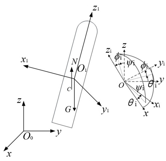
Figure 1.
Definition of two coordinate systems of the water-exit process.
In Figure 1, O1 is the barycenter, c is the center of buoyancy, G is gravity and N denotes the buoyancy. The coordinate transform matrix from O0x0y0z0 to O1x1y1z1 is given by
where φ, ψ and γ represent the pitch angle, yaw angle and roll angle for the submersible aerial vehicle. The momentum Q and moment of momentum K of the submersible aerial vehicle are described as follows:
Here, m is the mass of the submersible aerial vehicle and rc = [xc yc zc]T is the position vector of buoyancy in the body coordinate system. J0 = diag([Jx Jy Jz]) represents the rotational inertia matrix. By using the momentum theorem and the moment of momentum theorem, the dynamics model of the submersible aerial vehicle is described as
where Q is the linear momentum of rigid body, K is the angular momentum of rigid body, w is the angular velocity of rigid body, V is the linear velocity and Rc and Mc, respectively, denote the resultant force and moment of all external forces acting on the vehicle.
3.4. Polynomial Response Surface Model
The polynomial response surface model uses a polynomial to fit the design space, takes an algebraic polynomial as the basis function, uses the least squares method to calculate the coefficients of algebraic polynomial and then constructs the response surface model. The basic form of polynomial response surface model is shown in Equation (10):
where is an approximation of the response and are the parameters to be determined. Together, they form the polynomial parameter vector β. For β, the least squares method is used to solve:
Here, X is the vector formed by the x value of each sample point and Y is the vector formed by the y value of each sample point.
3.5. Boundary Conditions
The calculation domain is 9 m long, 7 m wide and 19.8 m high. The height of the liquid level from the bottom of the grid area is 9.5 m. Structured orthogonal grid cells are used to calculate the flow field. The calculation model uses nested grids containing a combination of two grid blocks. Grid block 1 includes the missile and its surrounding fluid area, which is 3.6 m long, 2.5 m wide and 17.7 m high. The length of the grid size is 0.04 m and the number of grids is 2.512 million. The scope of grid block 2 occupies the overall calculation area. The length of the grid size is 0.1 m and the number of grids is 1.25 million. The wave height of level 5 wave is 2.5 m, the period is 2.5 s and the wavelength is 14 m. The boundary condition of the overall calculation area is set as shown in Figure 2.
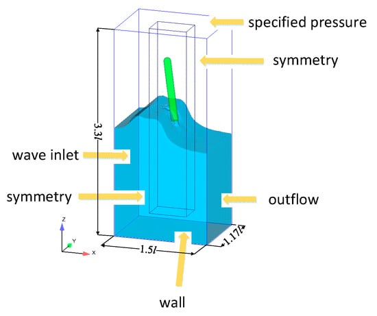
Figure 2.
Boundary condition type.
4. Simulation Model Validation
According to the above free surface model, the water-entry process of a rotating body was numerically simulated and the numerical results were compared with experiments [28] to verify the accuracy and effectiveness of the numerical method. The shape of the water-entry object is shown in Figure 3. The diameter of the rotating body was D0 = 9 mm, the length of the column section was L = 40 mm and the head was θ = 140° taper head type. The experimental model was made of ordinary steel with density ρ = 7.85 g/cm3. The initial inclination of the rotating body was 55° and the initial water-entry velocity was 4.35 m/s. The velocity direction of the rotating body was along the axis of the rotating body. Figure 4 shows the comparison between the experimental image and the simulation image of the inclined water-entry process of the rotating body. Figure 5 shows the comparison of the velocity of mass center and inclination angle.
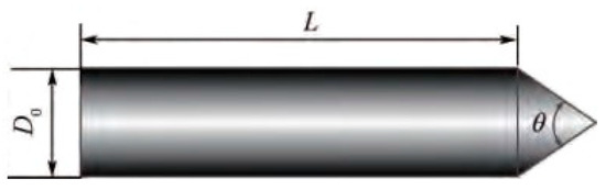
Figure 3.
Water-entry object.
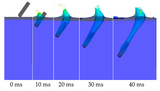
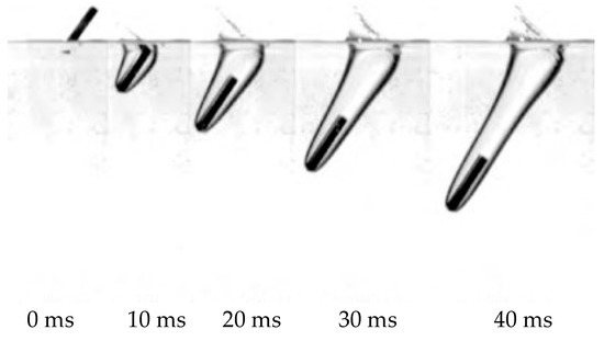
Figure 4.
Calculated results of velocity magnitude and high-speed photographs from experiments.
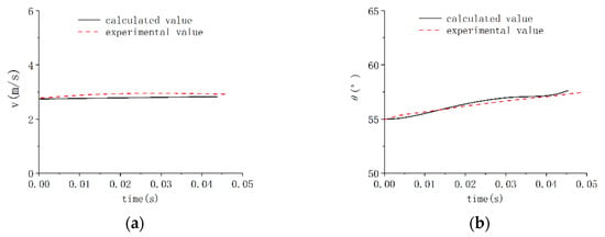
Figure 5.
Comparison of the velocity of mass center and inclination angle. (a) Velocity of mass center. (b) Angle of inclination.
5. Results and Discussion
To investigate the influence of initial inclination angle and launching velocity on the motion characteristics of the submersible aerial vehicle, we simulated the cross-medium water-exit process of submersible aerial vehicles under the conditions of different velocities and inclination angles. Images of a missile’s water-exit motion for the 9 cases considered are shown in Figure 6. With the movement of the missile, the missile head emerges from the water and the missile body crosses the water–air medium into the air. The wave beats the missile, causing disturbance to the missile’s water-exit process. The missile speed decreases, the free surface gradually breaks and, finally, the missile flies out of the water completely.
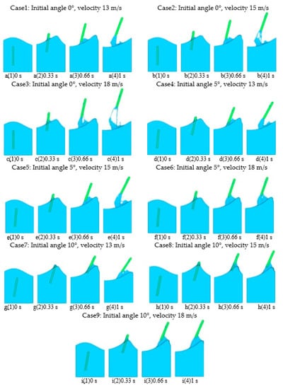
Figure 6.
Image of vehicle flying out of water.
5.1. Influence of Initial Inclination Angle
Figure 7, Figure 8 and Figure 9 show the comparison of mass center displacement of submersible aerial vehicles under three different inclination angles. Table 2 shows the centroid coordinates of the vehicle. Due to the influence of waves on the process of submersible aerial vehicle water-exit—the load fluctuation caused by cross-medium—the submersible aerial vehicle vibrates slightly in the X and Y directions. Under the condition of the same velocity and wave level at the time of flying out of the water, the displacement of the submersible aerial vehicle with an inclination angle of 10° is greater than that of 5° in the X direction and the displacement of the submersible aerial vehicle with an inclination angle of 5° is greater than that of 0° in the X direction. The displacements of submersible aerial vehicles in the Y direction are very small (<0.018 m) and the displacements in the Z direction are similar under the conditions of inclination angles of 10°, 5° and 0°.
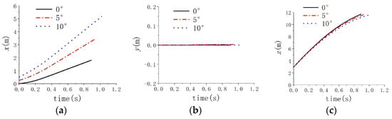
Figure 7.
Centroid coordinates of vehicle in case 1, 2, 3. (a) Vehicle centroid X-axis coordinates. (b) Vehicle centroid Y-axis coordinates. (c) Vehicle centroid Z-axis coordinates.
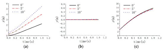
Figure 8.
Centroid coordinates of vehicle in case 4, 5, 6. (a) Vehicle centroid X-axis coordinates. (b) Vehicle centroid Y-axis coordinates. (c) Vehicle centroid Z-axis coordinates.
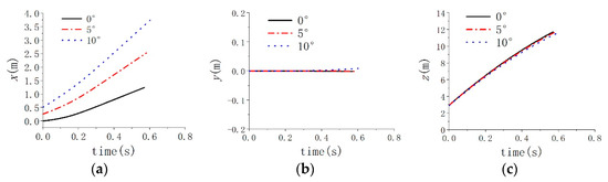
Figure 9.
Centroid coordinates of vehicle in case 7, 8, 9. (a) Vehicle centroid X-axis coordinates. (b) Vehicle centroid Y-axis coordinates. (c) Vehicle centroid Z-axis coordinates.
Table 2.
Centroid coordinates of vehicle.
Figure 10, Figure 11 and Figure 12 show the axial velocity variation of submersible aerial vehicles. During the whole moving process, the axial velocity decreases gradually and the missile finally flies out of the water and into the air trajectory. Under the condition of the same velocity and wave level at the time of flying out of the water, the variation trend of axial velocity of submersible aerial vehicles under the conditions of inclination angles of 10°, 5° and 0° is similar.
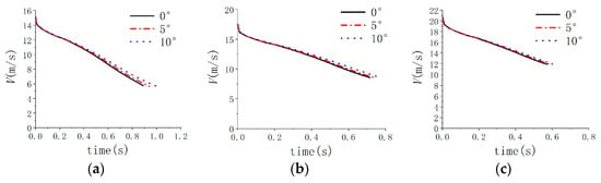
Figure 10.
Images of axial velocity variation of vehicle under different initial angles. (a) Axial velocity of vehicle in case 1, 2, 3. (b) Axial velocity of vehicle in case 4, 5, 6. (c) Axial velocity of vehicle in case 7, 8, 9.
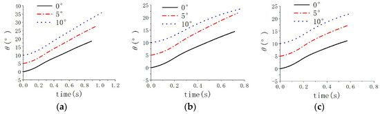
Figure 11.
Images of pitch angle variation of vehicle under different initial angles. (a) Pitch angle of vehicle in case 1, 2, 3. (b) Pitch angle of vehicle in case 4, 5, 6. (c) Pitch angle of vehicle in case 7, 8, 9.
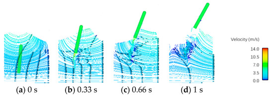
Figure 12.
Streamline diagram of vehicle flying out of water in case 2.
Figure 13, Figure 14 and Figure 15 show the attitude angle of submersible aerial vehicles during the process of submersible aerial vehicles flying out of the water. The pitch angles of the vehicle under various cases are shown in Table 3. The pitch angle at the time when the vehicle exits the water with an initial inclination of 10° is greater than the pitch angle with an initial inclination of 5° and the pitch angle at the time when the vehicle exits the water with an initial inclination of 5° is greater than the pitch angle with an initial inclination of 0°. As such, the inclination angle of 0° is more favorable to the vehicle’s water-exit process than 5° and the inclination angle of 5° is more favorable to the vehicle’s water-exit process than 10°.
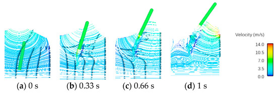
Figure 13.
Streamline diagram of vehicle flying out of water in case 3.
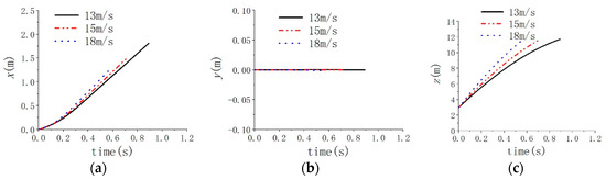
Figure 14.
Centroid coordinates of vehicle in case 1, 4, 7. (a) Vehicle centroid X-axis coordinates. (b) Vehicle centroid Y-axis coordinates. (c) Vehicle centroid Z-axis coordinates.
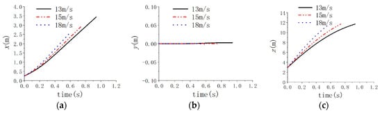
Figure 15.
Centroid coordinates of vehicle in case 2, 5, 8. (a) Vehicle centroid X-axis coordinates. (b) Vehicle centroid Y-axis coordinates. (c) Vehicle centroid Z-axis coordinates.
Table 3.
Pitch angle of vehicle.
According to Figure 16 and Figure 17, we can find that the underwater streamline moves to the right, the wave force on the vehicle moves to the right and the vehicle deflects to the right, leaving the water surface under the action of the wave. The flow velocity at the wave crest is the largest in the flow field distribution. During the motion of the vehicle in the water, vortices form at the tail of the vehicle, which makes the flow field near the vehicle change dramatically. The streamline velocity at the tail of the vehicle is greater than that of the surrounding flow field.
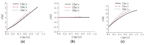
Figure 16.
Centroid coordinates of vehicle in case 3, 6, 9. (a) Vehicle centroid X-axis coordinates. (b) Vehicle centroid Y-axis Coordinates. (c) Vehicle centroid Z-axis coordinates.
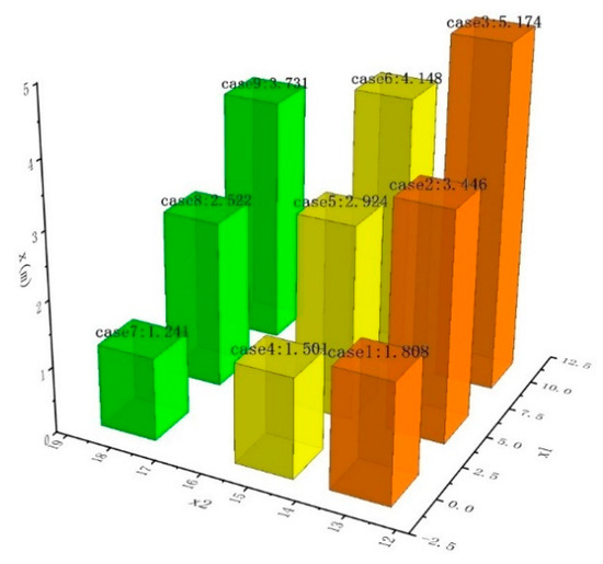
Figure 17.
Vehicle centroid X-axis coordinates at the end of the water-exit process of 9 cases.
5.2. Influence of Water-Exit Velocity on Submersible Aerial Vehicle’s Trans-Medium Motion
Figure 14, Figure 15 and Figure 16 show the comparison of mass center displacement of submersible aerial vehicle under three different velocities of water-exit. We can find that the displacement of the submersible aerial vehicle in X direction with a velocity of 13 m/s is greater than that of 15 m/s and the displacement of the submersible aerial vehicle in X direction with a velocity of 15 m/s is greater than that of 18 m/s, under the condition of the same inclination angle and wave level at the time of flying out of the water. In order to make a careful comparison, the vehicle centroid X-axis coordinates at the end of the water-exit process of 9 cases, with respect to the different initial inclination angle x1 and water-exit velocity x2, are shown in Figure 17. The displacements of submersible aerial vehicles in the Y direction are very small. The displacement of submersible aerial vehicles with initial velocities of 13 m/s, 15 m/s and 18 m/s are similar in Z direction.
The axial velocity of submersible aerial vehicle decreases gradually in the process of flying out of water, as shown in Figure 18 Under the condition of the same inclination angle and wave level at the time of flying out of the water, when the initial velocity is 13 m/s, the submersible aerial vehicle flies out of the water at about 0.93 s. When the initial velocity is 15 m/s, the vehicle flies out of the water at about 0.68 s. When the initial velocity is 18 m/s, the submersible aerial vehicle flies out of the water at about 0.55 s.
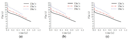
Figure 18.
Images of axial velocity variation of vehicles under different initial velocities. (a) Axial velocity of vehicle in case 1, 4, 7. (b) Axial velocity of vehicle in case 2, 5, 8. (c) Axial velocity of vehicle in case 3, 6, 9.
Figure 19 show the attitude angle of submersible aerial vehicle during the process of submersible aerial vehicles flying out of the water; the pitch angle of submersible aerial vehicles changes more at 13 m/s than at 15 m/s and the pitch angle of submersible aerial vehicles changes more at 15 m/s than at 18 m/s. As such, the water outlet velocity of 18 m/s is more favorable to the vehicle’s water-exit process than 15 m/s and the water outlet velocity of 15 m/s is more favorable to the vehicle’s water-exit process than 13 m/s. Thus, at the same initial inclination angle, the larger the initial velocity, the smaller the displacement and attitude angle changes of the submarine-launched vehicle [29].
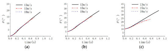
Figure 19.
Images of pitch angle variation of vehicles under different initial velocities. (a) Pitch angle of vehicle in case 1, 4, 7. (b) Pitch angle of vehicle in case 2, 5, 8. (c) Pitch angle of vehicle in case 3, 6, 9.
According to the streamlines of submersible aerial vehicles flying out of the water shown in Figure 20 and Figure 21 the direction of the streamlines points to the right. A vortex exists in the rear flow field of the vehicle. The smaller the initial velocity, the longer the vehicle will fly out of the water. The size of the vortex near the tail of the vehicle with larger initial velocity is larger and the corresponding velocity of the vortex is also larger.
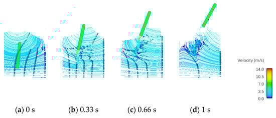
Figure 20.
Streamline diagram of vehicles flying out of water in case 2.
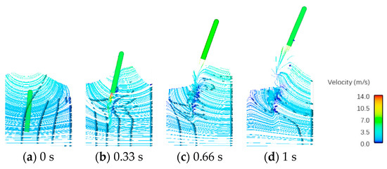
Figure 21.
Streamline diagram of vehicles flying out of water in case 8.
5.3. Submersible Aerial Vehicle’s Trans-Medium Motion Stability Analysis
It is necessary to analyze the stability of submarine aerial vehicles [30] in water-exit movement. The pitch angle plays an important role in the stability of a submersible aerial vehicle’s trans-medium motion. The trans-medium motion stability fitting function model of a submersible aerial vehicle is established based on the response surface model using the simulation data. Equation (11) represents the expression of the relationship between the pitch angle θ and both the inclination angle x1 and the water-exit velocity x2, when the wave-exit position is at the wave crest and the reference inclination angle is θ0 = 5°, as shown in Figure 22.
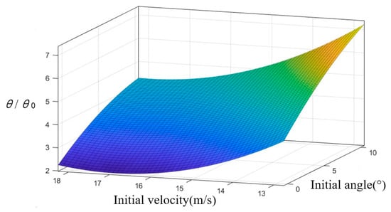
Figure 22.
Fitting function image of vehicle pitch angle θ with respect to inclination angle x1 and water-exit velocity x2.
Equation (12) shows the fitting function relationship of the submersible aerial vehicle velocity v at the end of the water-exit process with respect to the different initial inclination angle x1 and water-exit velocity x2 and the reference velocity is v0 = 15 m/s, as shown in Figure 23.
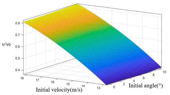
Figure 23.
Fitting function image of vehicle velocity v with respect to inclination angle x1 and water-exit velocity x2.
After establishing the response surface function model, given any group of inclination angle and velocity, the pitch angle of submersible aerial vehicles at the end of the water-exit process can be obtained. Next, the fitting function relationship established above is verified. When the initial inclination angle x1 is 8° and the initial velocity x2 is 14 m/s, using Equations (11) and (12) and relying on the established fitting function relationship, the predicted pitch angle and velocity are 27.56°and 7.39 m/s. The simulation calculation results are 27.27° for the pitch angle and 7.6 m/s for the velocity. The errors are less than 2.7%, so the correctness of the established fitting function relationship is verified.
At the same initial velocity of launch, the greater the initial inclination angle, the smaller the velocity at the end of submersible aerial vehicle’s water-exit process. Compared with the initial inclination angles of 0° and 5°, when the initial inclination angle is 10° and the water-exit velocity is 10.8 m/s, the velocity of the vehicle under the level 5 wave decreases to 0 at the end of the water-exit process, relying on the simulation analysis of submersible aerial vehicle water-exit movement. Therefore, the water-exit velocity of submersible aerial vehicles should be greater than 10.8 m/s to achieve successful launch. When the water-exit velocity of the vehicle is above 10.8 m/s, the smaller the initial inclination angle, the more favorable it is for the vehicle launch water-exit process. If the initial inclination angle is too large, the vehicle inclination angle may be too large at the end of the water-exit process and the launch will be unstable.
6. Conclusions
This paper establishes a multiphase coupling model for the motion across water–air media of submersible aerial vehicles to study the effects of various launch conditions and interference factors on the vehicle’s water-exit motion. The water-exit process under the conditions of different initial inclination angles and different velocities were simulated. The following conclusions can be derived through comparative analyses of 9 cases. Based on the comparison of the displacement, axial velocity, inclination angle change process and streamline diagram, the smaller the initial inclination angle, the more favorable the submarine-launched vehicle will be to the water-exit process. The initial inclination angle of 0° is the optimal initial angle for launching. In the limit range of the existing positive buoyancy, the optimal water-exit velocity of the submarine-launched vehicle is 18 m/s. Based on the established motion stability response function of the submersible aerial vehicle in the water-exit process, the pitch angle and velocity of the submersible aerial vehicle at the end of the water-exit process corresponding to any group of inclination angle and velocity can be solved, which can provide reference for the evaluation of submersible aerial vehicle launch safety. To achieve successful launch, the water-exit velocity of submersible aerial vehicles should be greater than 10.8 m/s. In the future, analysis can also be conducted on the influence of the initial inclination angle and velocity on the inclination angle and velocity of submarine aerial vehicles under different sea conditions when exiting the water. The water-exit movement stability of submarine aerial vehicles with different shapes can also be analyzed.
Author Contributions
Conceptualization, B.L.; data curation, X.C.; formal analysis, B.L. and E.L.; funding acquisition, G.L.; investigation, B.L.; methodology, B.L.; project administration, G.L.; resources, B.L.; software, B.L.; supervision, B.L.; validation, B.L.; visualization, B.L.; writing—original draft, B.L.; writing—review & editing, B.L. All authors have read and agreed to the published version of the manuscript.
Funding
This research received no external funding.
Institutional Review Board Statement
Not applicable.
Informed Consent Statement
Not applicable.
Data Availability Statement
Not applicable.
Conflicts of Interest
The authors declare no conflict of interest.
References
- Li, Y.G.; Wang, C.; Wu, Y.Y.; Cao, W.; Lu, J.X.; He, Q.K. On the motion characteristics of Cavity Wall in the High-speed Water Entry of Trans-media Vehicle. Acta Armamentari 2022, 43, 574–585. [Google Scholar]
- Truscott, T.T.; Epps, B.P.; Belden, J. Water Entry of Projectiles. Annu. Rev. Fluid Mech. 2014, 46, 355–378. [Google Scholar] [CrossRef]
- Lu, C.Y.; Wang, X.; Zhou, Z.T.; Liang, X.Y.; Le, G.G. Investigation on separating kinematic characteristics of submarine-launched missile near free surface. J. Astronaut. 2021, 42, 496–503. [Google Scholar]
- Lu, Y.L.; Hu, J.H.; Chen, G.M.; Liu, A.; Feng, J.F. Optimization of water-entry and water-exit maneuver trajectory for morphing unmanned aerial-underwater vehicle. Ocean Eng. 2022, 261, 112015. [Google Scholar] [CrossRef]
- Hu, K.; Ding, F.L. Simulated Research of Submarine Ballistic Missile Launching Movement Modeling and Manoeuvre Controll. Ship Sci. Technol. 2013, 35, 109–114. [Google Scholar]
- Bian, X.Y.; Zhao, X.P.; Zhu, C.B.; Li, X.L. Study on the influence of launch Parameters on the safety of vehicle trajectory. J. Ordnance Equip. Eng. 2017, 38, 40–45. [Google Scholar]
- Cao, J.Y.; Lu, C.J.; Chen, Y.; Chen, X.; Li, J. Research on the Base Cavity of a Sub-launched Projectile. J. Hydrodyn. 2012, 24, 244–249. [Google Scholar] [CrossRef]
- Shao, Z.W.; Han, P.W.; Ming, Y.; Lin, P.W.; Guang, W.W. Simulation on Three Dimensional Water-Exit Trajectory of Submersible Aerial Vehicle. Adv. Mater. Res. 2013, 2649, 791–793. [Google Scholar]
- Hu, J.H.; Xu, B.W.; Feng, J.F.; Qi, D.; Yang, J. Research on Water-Exit and Take-off Process for Morphing Unmanned Submersible Aerial Vehicle. China Ocean Eng. 2017, 31, 202–209. [Google Scholar] [CrossRef]
- Yuan, X.L.; Zhang, Y.W.; Duan, C.Y.; Liu, L.H. Water-Exit Trajectory Modeling and Experimental Validation of Unpowered Sub Launched Missile Carrier. J. Proj. Rocket. Missiles Guid. 2003, 23, 187–189. [Google Scholar]
- Siddall, R.; Kovac, M. Launching the AquaMAV: Bioinspired design for aerial–aquatic robotic platforms. Bioinspiration Biomim. 2014, 9, 031001. [Google Scholar] [CrossRef]
- Moshari, S.; Nikseresht, A.H.; Mehryar, R. Numerical analysis of two and three dimensional buoyancy driven water-exit of a circular cylinder. Int. J. Nav. Archit. Ocean Eng. 2014, 6, 219–235. [Google Scholar] [CrossRef]
- Chu, X.S.; Yan, K.; Wang, Z.; Zhang, K.; Feng, G. Numerical simulation of water-exit of a cylinder with cavities. In Proceedings of the International Conference on Hydrodynamics, ICHD-2010, China Ship Scientific Research Center, Wuxi, China, 21–25 October 2022. [Google Scholar]
- Ni, B.S.; Wu, G.X. Numerical simulation of water exit of an initially fully submerged buoyant spheroid in an axisymmetric flow. Fluid Dyn. Res. 2017, 49, 045511. [Google Scholar] [CrossRef]
- Xiao, M.; Shi, Z.K. Attitude control and trajectory simulation in the process of a mine out of water. Acta Armamentarii 2010, 31, 1151–1156. [Google Scholar]
- Wu, Q.G.; Ni, B.Y.; Xue, Y.Z.; Zhang, A.M. Experimental and numerical study of free water exit and re-entry of a fully submerged buoyant spheroid. Appl. Ocean Res. 2018, 76, 110–124. [Google Scholar] [CrossRef]
- Zhang, H.S.; Zhang, Z.L.; He, F.; Liu, M.B. Numerical investigation on the water entry of a 3D circular cylinder based on a GPU-accelerated SPH method. Eur. J. Mech. B/Fluids 2022, 94, 1–16. [Google Scholar] [CrossRef]
- Bhalla, A.P.S.; Nangia, N.; Dafnakis, P.; Bracco, G.; Mattiazzo, G. Simulating water-entry/exit problems using Eulerian–Lagrangian and fully-Eulerian fictitious domain methods within the open-source IBAMR library. Appl. Ocean Res. 2020, 94, 101932. [Google Scholar] [CrossRef]
- Vinod, V. Nair; S.K. Bhattacharyya. Water entry and exit of axisymmetric bodies by CFD approach. J. Ocean Eng. Sci. 2018, 3, 156–174. [Google Scholar]
- Wu, G.X. Hydrodynamic force on a rigid body during impact with liquid. J. Fluids Struct. 1998, 12, 549–559. [Google Scholar] [CrossRef]
- Zhao, C.G.; Wang, C.; Wei, Y.J.; Zhang, X.S.; Sun, T.Z. Experimental study on oblique water entry of projectiles. Mod. Phys. Lett. B 2016, 30, 1650348. [Google Scholar] [CrossRef]
- Tassin, A.; Piro, D.J.; Korobkin, A.A.; Maki, K.J.; Cooker, M.J. Two-dimensional water entry and exit of a body whose shape varies in time. J. Fluids Struct. 2013, 40, 317–336. [Google Scholar] [CrossRef]
- Ma, Z.C.; Hu, J.H.; Feng, J.F.; Liu, A.; Chen, G.M. A longitudinal air-water trans-media dynamic model for slender vehicles under low-speed condition. Nonlinear Dyn. 2020, 99, 1195–1210. [Google Scholar] [CrossRef]
- Huang, L.; Tavakoli, S.; Li, M.; Dolatshah, A.; Pena, B.; Ding, B.; Dashtimanesh, A. CFD analyses on the water entry process of a freefall lifeboat. Ocean. Eng. 2021, 232, 109115. [Google Scholar] [CrossRef]
- Budiarso; Siswantara, A.I.; Darmawan, S.; Tanujaya, H. Inverse-Turbulent Prandtl Number Effects on Reynolds Numbers of RNG k-ε Turbulence Model on Cylindrical-Curved Pipe. Appl. Mech. Mater. 2015, 3918, 758. [Google Scholar]
- Issac, J.; Singh, D.; Kango, S. Experimental and numerical investigation of heat transfer characteristics of jet impingement on a flat plate. Heat Mass Transf. Wärme-Und Stoffübertragung 2020, 56, 531–546. [Google Scholar] [CrossRef]
- Hirt, C.W.; Nichols, B.D. Volume of fluid (VOF) method for the dynamics of free boundaries. J. Comput. Phys. 1981, 39, 201–225. [Google Scholar] [CrossRef]
- Song, W.C.; Wang, C.; Wei, Y.J.; Xu, H. Experiment of cavity and trajectory characteristics of oblique water entry of revolution bodies. J. Beijing Univ. Aeronaut. Astronaut. 2016, 42, 2386–2394. [Google Scholar]
- Liu, B.; Liu, K.; Xue, R.J.; Zhang, L.Y.; Le, G.G. Research on separation of submarine-launched missile with elastic adapter. J. Ordnance Equip. Eng. 2022, 43, 136–144. [Google Scholar]
- Du, X.X.; Song, B.W.; Hu, H.B.; Wang, P. Simulation of submarine-aerial missile carrier’s water- trajectory. Syst. Eng. Theory Pract. 2007, 10, 172–176. [Google Scholar]
Disclaimer/Publisher’s Note: The statements, opinions and data contained in all publications are solely those of the individual author(s) and contributor(s) and not of MDPI and/or the editor(s). MDPI and/or the editor(s) disclaim responsibility for any injury to people or property resulting from any ideas, methods, instructions or products referred to in the content. |
© 2023 by the authors. Licensee MDPI, Basel, Switzerland. This article is an open access article distributed under the terms and conditions of the Creative Commons Attribution (CC BY) license (https://creativecommons.org/licenses/by/4.0/).