Article

A Novel Method for Imputing Missing Values in Ship Static Data Based on Generative Adversarial Networks

College of Information Engineering, Shanghai Maritime University, Shanghai 201306, China
*
Author to whom correspondence should be addressed.
J. Mar. Sci. Eng. 2023, 11(4), 806; https://doi.org/10.3390/jmse11040806
Submission received: 11 March 2023 / Revised: 31 March 2023 / Accepted: 6 April 2023 / Published: 10 April 2023
(This article belongs to the Section Ocean Engineering)

Abstract

:
Ship data obtained through the maritime sector will inevitably have missing values and outliers, which will adversely affect the subsequent study. Many existing methods for missing data imputation cannot meet the requirements of ship data quality, especially in cases of high missing rates. In this paper, a missing data imputation method based on generative adversarial networks (GANs) is proposed. The generative adversarial imputation network (GAIN) is improved using the Wasserstein distance and gradient penalty to handle missing values. Meanwhile, the data preprocessing process is optimized by combining knowledge from the ship domain, such as using isolation forests for anomaly detection. Statistical analysis of ship data is also conducted, including correlation analysis of ship design parameters, analysis of outliers, and analysis of missing data types. These analyses provide the basis for the proposed model. In a case study of 8167 bulk carriers, the proposed model outperformed the missing forest (MF) and polynomial fitting (PF) models, with an average error reduction of 2.4% and 6.3%, respectively. The proposed model also showed stable performance in cases of high missing rates. This study provides a new approach for estimating or imputing critical parameters of ships.

1. Introduction

As a means of transportation and transport equipment, ships have always been an indispensable infrastructure in certain areas, such as international trade, tourism, and defense and security [1]. With the continuous progress of technology, the performance and data collection capability of ships have been improved, but the problem of missing ship data still exists. These problems of missing data, which may be due to sensor failure, human error, aging equipment, or other reasons, negatively affect the safety and reliability of the ship [2,3]. In the past few decades, the shipping industry has been working to address the issue of missing ship data, including the development of more advanced sensor technologies, improving data collection and analysis methods, and promoting standardized data formats [4,5]. However, missing ship data are still an unavoidable problem due to certain factors, such as the complexity and diversity of ships and the cost of data collection and processing. Therefore, how to effectively deal with the problem of missing ship data to ensure the safety and performance of ships has been the focus of the shipping industry and the maritime field.
Although dealing with missing data has become one of the hot topics of research in the field of data analysis, there are not many in-depth studies or much research on the missing data of ships. The existing studies are mainly based on the analysis of AIS dynamic data, for example, by analyzing incomplete datasets to recover lost ship tracks or ship navigation status [6,7,8,9]. Shaoqing Guo et al. combined the distribution of time intervals and ship kinematic characteristics to propose a trajectory reconstruction method, which can effectively reconstruct the ship trajectory with higher performance [10]. Da-Wei Gao et al. introduced physical assumptions to balance complexity and accuracy and combined the advantages of the trajectory proposal network (TPNet) and long short-term memory (LSTM) to design a ship track prediction method that can be used for high-precision real-time analysis [11]. Michail Cheliotis et al. developed a new hybrid interpolation method for improving the quality of ship dynamic data by combining k-nearest neighbors (KNNs) and multiple imputation by chained equations (MICE) [12]. Gao et al. proposed a trajectory simplification algorithm based on ship navigation status and acceleration changes, which can combine with the main engine power to obtain key information about ship trajectory. They further analyzed the deep relationship between ship dynamic data and static data [13]. Research on missing data has mainly focused on ship dynamic data with time-series characteristics, but little research has been performed on ship static data.
Ship static data includes basic information about the ship, ship size, navigation attributes, and equipment parameters, which are important for the management, operation, and safety of the ship [14]. Current research in this area has focused on regression analysis of specific ship design parameters. Chen et al. obtained an approximate value by referring to the main engine power of ships with similar hull types, ship sizes, and total tonnage. However, this method cannot provide a reference if the basic attributes of the target ship are not available [15]. Huang et al. conducted a correlation analysis between host power and ship attributes and proposed a method for estimating host power based on ship resistance [16]. Abramowski et al. proposed a regression formula for estimating multiple design parameters of container ships, which was practically applied in the preliminary design stage and contributed to the development of ship design theory [17]. Gurgen et al. developed an artificial neural network (ANN) model with deadweight and ship speed as input layers and overall length, the length between drogue lines, width, draft, and drywall as output layers for predicting the main details of chemical ships in the preliminary design phase [18]. Youngrong Kim et al. proposed a model-based regression analysis method to deal with missing values and conducted a case study on the primary data of container ships, and the study showed the good applicability of the method to certain size-constrained ships [18]. However, the relationships among ship design parameters are complex, and it is difficult to reflect the deep connections among the parameters using only regression analysis. The applicability of the fitted curves is also difficult to guarantee due to the variety of ship types and different missing rates. It is worth noting that if key feature parameters are missing in the dataset, then these methods cannot be applied.
The deep learning model generative adversarial network (GAN) has received a lot of attention since its proposal, and many studies have improved it and applied it to different areas [19,20,21,22,23,24,25,26,27,28]. Poudevigne-Durance et al. propose a novel generative adversarial network (GAN) called MaWGAN (for masked Wasserstein GAN), which creates synthetic data directly from datasets with missing values easily implemented using masks generated from the pattern of missing data in the original dataset [26]. Nadimi-Shahraki et al. introduced a four-layer model and then proposed a hybrid imputation (HIMP) method using this model to impute multi-pattern missing data, including non-random, random, and completely random patterns [27]. Gulrajani et al. proposed an alternative to weight clipping: penalizing the norm of the critic’s gradient concerning its input. This improved the Wasserstein GAN (WGAN) which sometimes still generated low-quality samples or failed to converge. This also provided a new direction for GAN series models in missing data processing [28]. Jinsung Yoon et al. proposed a generative adversarial imputation net (GAIN) with high applicability to different types of missing datasets [29]. The method fills in the missing data by learning both the true distribution of samples and the distribution of missing values using the generator G and discriminator D of GAN. Compared with traditional imputation and regression methods, GAIN can better handle complex data distributions and nonlinear relationships while preserving data characteristics. GAIN and variants of GAIN have been used in a wide variety of data science and machine learning tasks other than in the maritime domain [30,31,32,33,34].
This study proposes a new method for ship missing data imputation based on generative adversarial networks (GANs). The method combines the relevant characteristics of ship data and improves upon GAIN to design a new imputation model, WFGAIN-GP, which can be widely applied to missing data processing for ship static data. The improvements include three aspects. Firstly, using polynomial fitting values as temporary filling values enables the model to learn the feature distribution of ship data more easily. Secondly, introducing the Wasserstein distance instead of JS divergence to measure the distance between the generated data distribution and the true data distribution improves the stability of the model. Thirdly, adding gradient penalty (GP) further improves the gradient vanishing or explosion problem in the model. In the data preprocessing stage, this study also proposes combining ship domain knowledge and an isolation forest (IF) to detect anomalies in the original data. In addition, the study analyzes the correlation, anomaly values, and missing types of ship data. Section 2 provides a detailed description of the new ship missing data imputation method. Section 3 demonstrates the model’s results through a case study of bulk carriers and compares its performance with GAIN, polynomial fitting models, and missing forest models. Finally, Section 4 summarizes the study.

2. Methodology

2.1. Missing Data Handling Process

In this study, a novel method for interpolating missing values in ship static data based on GAN is proposed, which can be widely applied to the processing of missing static data of ships. The model estimates the data based on the entire dataset through a generative and adversarial approach. It combines the relevant characteristics of ship data but does not rely on specific ship features. Therefore, this model can be applied to datasets with different types of ships and different features. In addition, this study used an isolation forest (IF) to design an outlier detection method and optimize data preprocessing. Figure 1 illustrates the proposed method in this study, with the main steps consisting of the following three steps.
Determine the imputation part: There are three types of data to be interpolated, namely non-regular input data, missing value data, and outlier data. The non-regular input data refers to the data containing non-compliant characters, which can be discerned based on the data format. The determination of outliers is more complex and needs to be determined analytically. In this study, the outliers are detected by combining the knowledge of the ship domain and the isolation forest (IF). Section 2.3 will describe the outlier detection method. The pseudo code is shown in Algorithm 1.
Algorithm 1: Determining the portion of data that needs to be imputed
1:for  i 1 , 2 , N  do
2: for  j 1 , 2 , M  do
3:  if  x i j is irregular input data, missing value data, or abnormal value data
4:   Set x i j to null.
5:    m i j = 0
6:  Else
7:    m i j = 1
8:  end if
9: end for
10:end for
where x i j is the data value of the j th parameter in the i th ship case. m i j is the mask value of the j th parameter in the i th ship case.
Missing value imputation: Firstly, it is necessary to temporarily fill in the missing values’ positions to facilitate subsequent data processing. This filling scheme outputs an approximation by a polynomial fitting function as a temporary filling value. Next, the incomplete dataset, the imputed dataset, and the mask vectors will be inputted into the proposed WFGAIN-GP model for analysis in this study. In this model, generator G observes some real data and uses the real data to predict the missing data and to output the complete data. Discriminator D attempts to determine which values in the complete dataset are observed real values and which ones are imputed values. At the end of the iteration, generator G generates high-quality predictions to replace the temporary fill values from the previous step. The details of the model are described in Section 2.2. The pseudo code is shown in Algorithm 2.
Algorithm 2: Impute missing values
1:/*Temporary filling */
2:for  i 1 , 2 , N  do
3:for j 1 , 2 , M  do
4:  if  x i j  is null
5:   Determine the available F j with the maximum R 2 value.
6:   Set  x ˜ i j to the f i j of F j .
7:  Else
8:  Set  x ˜ i j to the x i j .
9:  end if
10:end for
11:end for
12:/*Imputation*/
13:Input: Incomplete dataset X ˜ , Mask vector M .
14:for number of training iterations do
15:for k steps do
16:  Train the discriminator D.
17:end for
18: Train the Generator G.
19:end for
20:Output: Complete dataset
where  x i j is the data value of the j th parameter in the i th ship case. m i j is the mask value of the mask vector M . f i j is the fitted value of the polynomial fitting function F j x ˜ i j belongs to the imputed complete dataset X ˜ after temporary filling.
Final adjustment: Finally, this study references outlier detection standards as the normal range for imputed values to identify and correct unreasonable values. Some values identified as unreasonable need to be re-estimated or replaced with other values estimated in previous steps. The pseudo code is shown in Algorithm 3.
Algorithm 3: Adjusting predicted values with ship domain knowledge
1:for  i 1 , 2 , N  do
2:for  j 1 , 2 , M  do
3:  if  m i j = 0 and x i j is abnormal value data
4:   Re-estimate the value of x i j . or replace with the f i j .
5:   end if
6:end for
7:end for
where   x i j is the data value of the j th parameter in i th ship case. m i j is the mask value of the j th parameter in i th ship case. f i j is the fitted value of the polynomial fitting function F j .

2.2. WFGAIN-GP

This section proposes a new imputation model: the Wasserstein fitting GAIN with gradient penalty (WFGAIN-GP). The GAN model typically minimizes the Jensen–Shannon Divergence (JSD), a symmetric distance metric that measures the similarity between two distributions, namely between the generated data distribution and the real data distribution during training [30]. However, due to the possibility of vanishing gradients in certain cases, such as when using JSD, problems with gradient disappearance may arise during the training process [33]. The generator G and the discriminator D used in the GAIN model proposed by Jinsung Yoon et al. (2018) are based on GAN, so there are also problems of gradient disappearance and mode collapse during training. To make the model more stable and suitable for ship data characteristics, this study improved the GAIN model.
First, it is necessary to calculate the coefficient of determination ( R 2 ) between each parameter of the ship. Then, for each parameter and the one with the highest R 2 value, a polynomial fitting function is established, as shown in Equation (1). If a certain ship lacks the corresponding parameter value with the highest R 2 value, the next variable with the highest R 2 value is selected until the missing value is filled. GAIN utilizes random noise as temporary fill values, which injects noise into the generator network to help the network learn more potential patterns and data distribution information and improve its filling effect. Noise filling can also prevent the network from overfitting missing data, thereby improving its generalization performance. By using different noise distributions and sizes, the effect of noise filling can be further adjusted to meet different types and degrees of data missingness. In this study, a filling strategy that uses values closer to the true data is used as temporary imputed values, allowing the model to learn the feature distribution of ship data more easily. Secondly, this study introduces the Wasserstein distance from the Wasserstein GAN (WGAN) to measure the distance between the generated data distribution and the real data distribution, replacing the JSD used in the original GAN. The Wasserstein distance considers the structural information between two distributions, making it more robust to noise, outliers, and other exceptional situations, and can avoid the mode collapse problem associated with JSD in traditional GANs, thereby improving training stability [22]. Finally, to further improve the gradient vanishing or exploding issues in the model, we consider adding gradient penalty (GP) and gradient clipping (CP) to restrict the gradient. CP is a method that limits the gradient after it is computed by clipping the norm of the gradient vector to ensure that the length of the gradient vector does not exceed a given threshold. GP dynamically keeps the gradient norm of the discriminator within a reasonable range by computing the square of the gradient norm and adding it to the discriminator’s loss function. Due to the complex and diverse types of features in ship data, it is difficult to achieve a balance in the model through fixed threshold constraints, so GP is chosen to improve gradient issues. Figure 2 shows the framework diagram of the WFGAIN-GP model. Equation (1) is as follows:
y = i = 0 n k i · x i
where y is the design parameter, x is the parameter selected with suitable R 2 value, k i is the coefficient for each x i , and n represents the highest degree of the function.
Let χ = X 1 , X 2 , , X N     R d be an incomplete dataset. Let M = m 1 , , m d be a random variable taking values in 0 , 1 d , referred to as the mask vector, corresponding to each X χ . It reflects which variables are original data and which are imputed data. F represents a d-dimensional imputation vector (temporary imputed values).
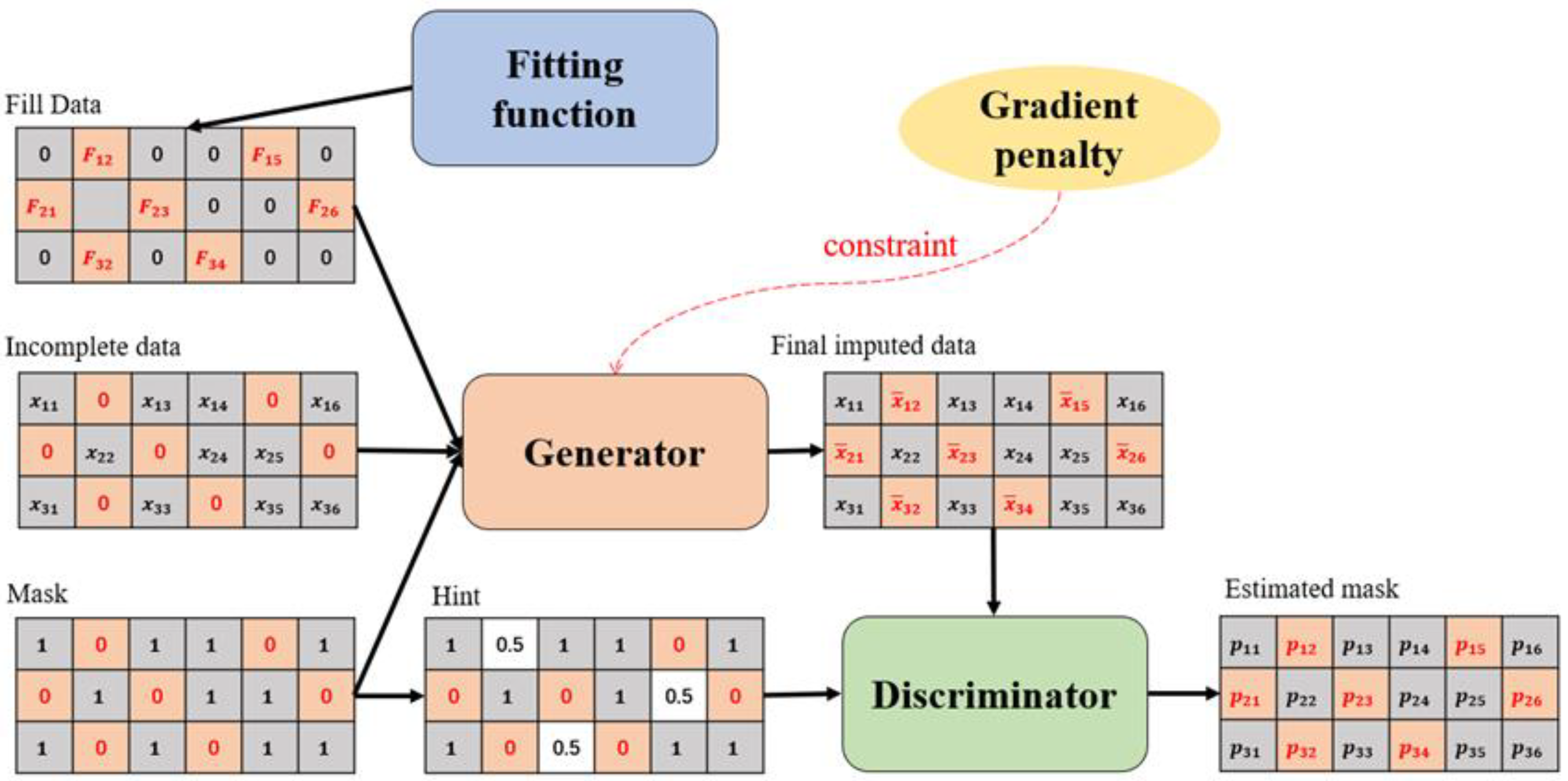
In addition, GAIN proposes the introduction of a hint mechanism to reinforce the adversarial process between G and D and to avoid G reproducing multiple optimal distributions. The hint mechanism is an artificially defined random variable H . The goal of the imputation process is to estimate the values of all missing positions in each X χ . Here, we try to find a data distribution model, rather than just its expected value. With multiple imputations, we can control the inherent uncertainty of the data. Figure 2 shows the framework of this model. The temporarily imputed data, original data, and mask are input to the generator, which outputs the imputed complete data under the constraint of gradient penalty. D receives the masked data processed by the hint mechanism and the complete data generated by G, and then outputs the discrimination result, i.e., a new mask.
G takes the incomplete dataset, imputed dataset, and mask vector as inputs, and outputs complete samples. The output of G can be represented as follows:
X ¯ = G X , M , 1 M F
X ^ = M X + 1 M X ¯
where X ¯ refers to the imputed values vector, excluding the observed data portion, and represents the Hadamard product. It should be noted that G outputs a value for each part, even if some parts are not missing. X ^ refers to the imputed complete data vector, which observes the local information of X , and then replaces the corresponding temporary imputed values with the estimated values from X ¯ .
D is used to train G as an adversary. The output of G consists of some parts that are real and some parts that are generated. D does not identify the truthfulness of the entire vector but tries to discriminate which parts are real and which parts are generated. This is equivalent to predicting the m values in the mask vector M . Therefore, the output of D is a binary vector, represented as follows:
M ^ = D X ^ , H
where M ^ is the predicted vector of the mask vector M .
The objective of WFGAIN-GP is customized as follows:
min D 1 N k = 1 N L D M k , M D k + λ · GP
min G 1 N k = 1 N L G M k , M D k + α L M X k , X M k
where α and λ are hyperparameters. GP is the gradient penalty term, which can dynamically constrain the growth rate of D. In the original GAIN, the specific definition of the objective function is based on JS divergence, and L D L and L G are defined as follows:
L D M , M D = M · log M D 1 M · log 1 M D
L G M , M D = 1 M · log M D
However, this definition has some problems. In simple terms, the better D is trained, the more severe the gradient disappearance of G is. When there is no overlap between the real sample distribution P r and the sample distribution P g generated by G, or the overlap part can be ignored, the gradient in the gradient descent method is zero. At this time, for D under the approximate optimal condition, G cannot obtain any gradient information, and the problem of gradient disappearance is likely to occur. When the support set of P r and P g is a low-dimensional manifold in high-dimensional space, the probability that the overlap part has a measure of zero is one [22]. Therefore, the possibility of P r and P g not overlapping or the overlapping part being negligible is very high. The hint mechanism proposed by the authors of GAIN resembles a transitional solution from GAN to WGAN (adding high-dimensional noise), which can force them to have a non-negligible overlap to some extent. However, it is still difficult to determine a numerical indicator to measure the training progress, while the Wasserstein distance can solve this problem.
The Wasserstein distance is defined as follows:
W P r , P g = i n f γ P r , P g E x , y ~ γ x y
where P r , P g is the set of all possible joint distributions of the combined P r and P g distributions. For each possible joint distribution γ , a sample x and y can be sampled from it to calculate the distance between the sample pair x y , so the expected value E x , y ~ γ x y of the sample pair distance can be calculated under this joint distribution γ . The lower bound of this expected value that can be achieved among all possible joint distributions is the Wasserstein distance.
However, the i n f γ P r , P g in Equation (9) cannot be directly solved and, in the WGAN paper, it was transformed into a solvable equation through derivation, and a new objective function was defined. Compared with GAN, WGAN modifies the following four aspects:
  • Removes the sigmoid activation function in the last layer of D.
  • Removes the log from the loss functions of G and D.
  • After updating the parameters of D each time, truncates so that their absolute values do not exceed a fixed constant.
  • Uses RMSProp or SGD instead of momentum-based optimization algorithms.
  • Therefore, based on the third modification, the new L D and L G are defined as follows:
L D M , M D = M · M D 1 M · 1 M D
L G M , M D = 1 M · M D
L M is defined as follows:
L M X , X = i = 1 d m i · x i x i 2
As can be seen from the definition, L G applies to missing components ( m i = 0 ), while L M applies to observed components ( m i = 1 ). L G M , M D is minimized when discriminator D incorrectly classifies the imputed values as observed. L M X , X is minimized when the non-missing values output by generator G approach the actual observed values.

2.3. Detection of Outliers

This study combines two methods to determine outliers. First, the outlier detection criteria were established based on the specific value ranges of ship-related attributes provided by the International Maritime Organization’s Fourth Greenhouse Gas Study report [35]. The outlier detection criteria for each design parameter are shown in Table 1. The simple interval division allows for the quick identification of more obvious outliers. Then, the isolation forest (IF) is used to detect the outliers whose features are within the normal range but whose overall ship parameters are abnormal. IF is an unsupervised machine learning algorithm used for anomaly detection and can be used to detect outliers in a dataset. The IF algorithm first randomly partitions the dataset into multiple subsets and builds a random forest (RF) for each subset. Then, for each sample point, the IF algorithm finds a path in the RF, and the length of the path is the average distance between the sample point and other sample points in the RF. This length can be used as the anomaly score for the sample point, and if the score is greater than a given threshold, the sample point is considered an anomaly.

2.4. Experimental Evaluation Criteria

To evaluate the performance of the proposed imputation method in the application of ship static data, this study used three statistical indicators: root mean square error (RMSE), mean absolute percentage error (MAPE), and area under the receiver operating characteristic curve (AUROC), to evaluate the imputation results. The smaller the value, the better the imputation effect, and vice versa. In addition, the coefficient of determination ( R 2 ) was used to analyze the imputation process. The formulae are as follows:
RMSE = 1 N i = 1 N x i x ^ i 2
MAPE = 100 N i = 1 N x i x ^ i x i %
ρ X ,   Y = E X μ X Y μ Y σ X σ Y
R 2 = 1 i = 1 N x i x ^ i 2 i = 1 N x i x i ¯ 2
where x i represents the observed value of the dependent variable, x ^ i represents the predicted value of the dependent variable, x i ¯ represents the mean value of the observed data, and RSS represents the residual sum of squares. ρ X ,   Y is the correlation coefficient between variables X and Y, E is the expected value operator, and σ X and σ Y are the standard deviations.

3. Case Study

This chapter will analyze a specific case study. Section 3.1 conducts statistical analysis on the correlation, outliers, and missing types of ship design parameters. Section 3.2 performs regression fitting between ship design parameters to provide a basis for the proposed imputation scheme. Section 3.3 compares the proposed model with three other models to validate its applicability. Section 3.4 discusses the imputation performance of the model under different feature dimensions. Section 3.5 performs imputation and analysis on real missing data.

3.1. Ship Database Analysis

The static ship data used in this study were obtained from Clarkson and Lloyd’s databases, with all vessels registered in China. The dataset includes 10 design parameters, which are ship length (L), breadth (B), molded depth (MD), main engine power (MEP), auxiliary engine power (AEP), boiler power (BP), rated speed (V), gross tonnage (GT), deadweight tonnage (DWT), and net tonnage (NT). In the case study, a dataset of bulk carriers was extracted, including 8,167 bulk carriers built between the earliest year, 1979, and the latest year, 2020. Statistical analysis of container and oil tanker data is provided in Appendix A and Appendix B, respectively. Statistical analysis includes correlation analysis, outlier analysis, and analysis of missing data types for ship design parameters. The correlation analysis provides a basis for subsequent polynomial fitting. Outlier analysis can optimize data preprocessing, and determining the types of missing data helps to better understand the reasons for data loss.
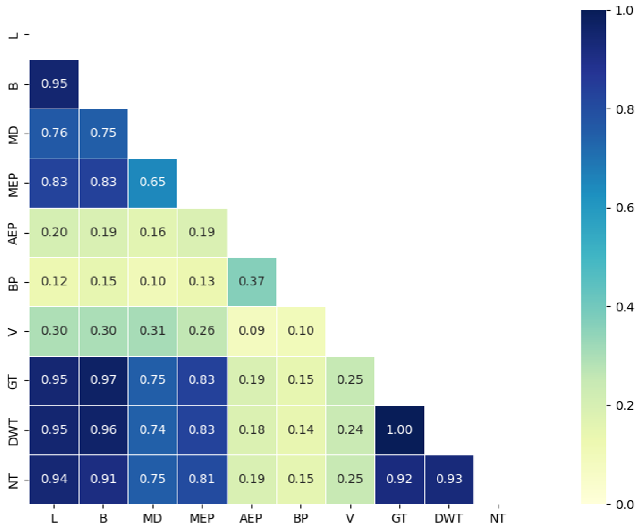
Table 2 and Table 3 provide descriptive statistics for each design parameter, where L, GT, DWT, and NT have relatively few missing values, while AEP has the highest number of missing values. The missing data accounts for 11.85% of the total data, and 59.01% of the total ships have missing data. Each ship has a maximum of five missing design parameters, and there are no ships with all design parameters missing. Therefore, the filling plan proposed in this study is feasible. This study conducted an R 2 analysis on all available data, and the results of the analysis for the ship design parameters are shown in Figure 3. In Figure 3, darker colors indicate higher goodness of fit or stronger correlation. Generally, if R 2 is greater than or equal to 0.7, it can be considered a strong correlation between the two variables. If R 2 is less than 0.3, it can be considered that there is a weak or no correlation between the two variables. When R 2 is between 0.3 and 0.7, there is a certain degree of correlation between the two variables, but further analysis is needed to determine the direction and strength of the correlation. The analysis clearly shows that there is a high degree of correlation (with R 2 values exceeding 0.9) among L, B, GT, DWT, and NT of bulk carriers. DWT and GT have a goodness of fit of 0.9993, indicating a very high correlation. There are also some correlations between V and BP with most of the other parameters, although with smaller R 2 values. The correlation between design parameters provides a basis for the imputation method proposed in this study.
Data missingness can be categorized into three types: missing completely at random (MCAR), missing at random (MAR), and missing not at random (MNAR) [36]. MCAR refers to missing data that occur randomly and are not related to any incomplete or completely observed variables. MAR refers to missing data that are not completely random, meaning that the missingness of this type of data is dependent on other fully observed variables. MNAR refers to missing data that are dependent on the incompletely observed variables themselves. To determine the type of missingness in the dataset, Little’s MCAR test was performed in this study. This is a commonly used method to determine whether the missing data type is MCAR based on the p value [37]. Table 4 shows the results of Little’s MCAR test on the dataset. According to the test performed on the current dataset, the p-value suggests that the data under investigation are not missing completely at random. This may be because the missing data are related to other complete variables, rather than being completely random. For example, some data may have been missed due to technical issues or operational errors during the data collection process. Additionally, ship operators may choose not to provide certain data, which is also not completely random when it is missing.
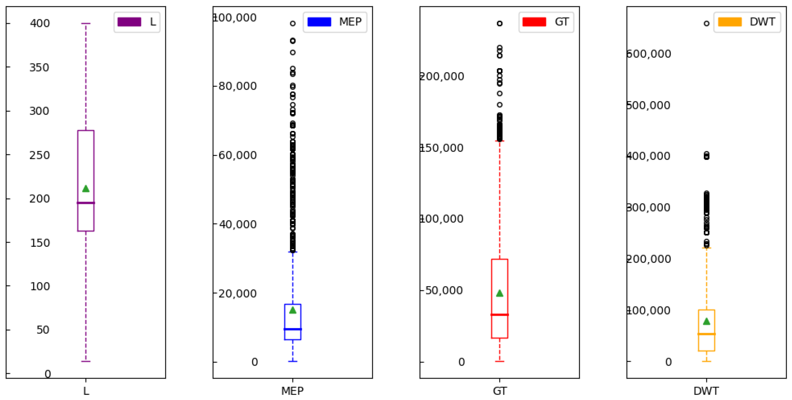
In statistics, kurtosis measures the peakedness of the probability distribution of a real-valued random variable. High kurtosis indicates that the increase in variance is caused by extreme deviations that occur infrequently. In Table 2, the kurtosis coefficients of AEP, MEP, BP, DWT, and GT are all greater than 3, indicating that these parameters require special attention. In the correlation analysis, MEP, DWT, and GT exhibit high correlations with L and B. Figure 4 shows box plots of the descriptive statistics of the raw data. The box plot of L does not display any outliers, while the box plots of MEP, DWT, and GT show a significant number of outliers. Therefore, in identifying outliers using the IF method, this study prioritizes using L and B as discriminant features and uses a dichotomous approach in the selection of values, dividing all ships into several small intervals through a binary tree. Then, MEP, DWT, and GT are used as the discriminating features, and values within a random range are selected to determine the outliers of these three parameters.

3.2. Polynomial Fit Analysis

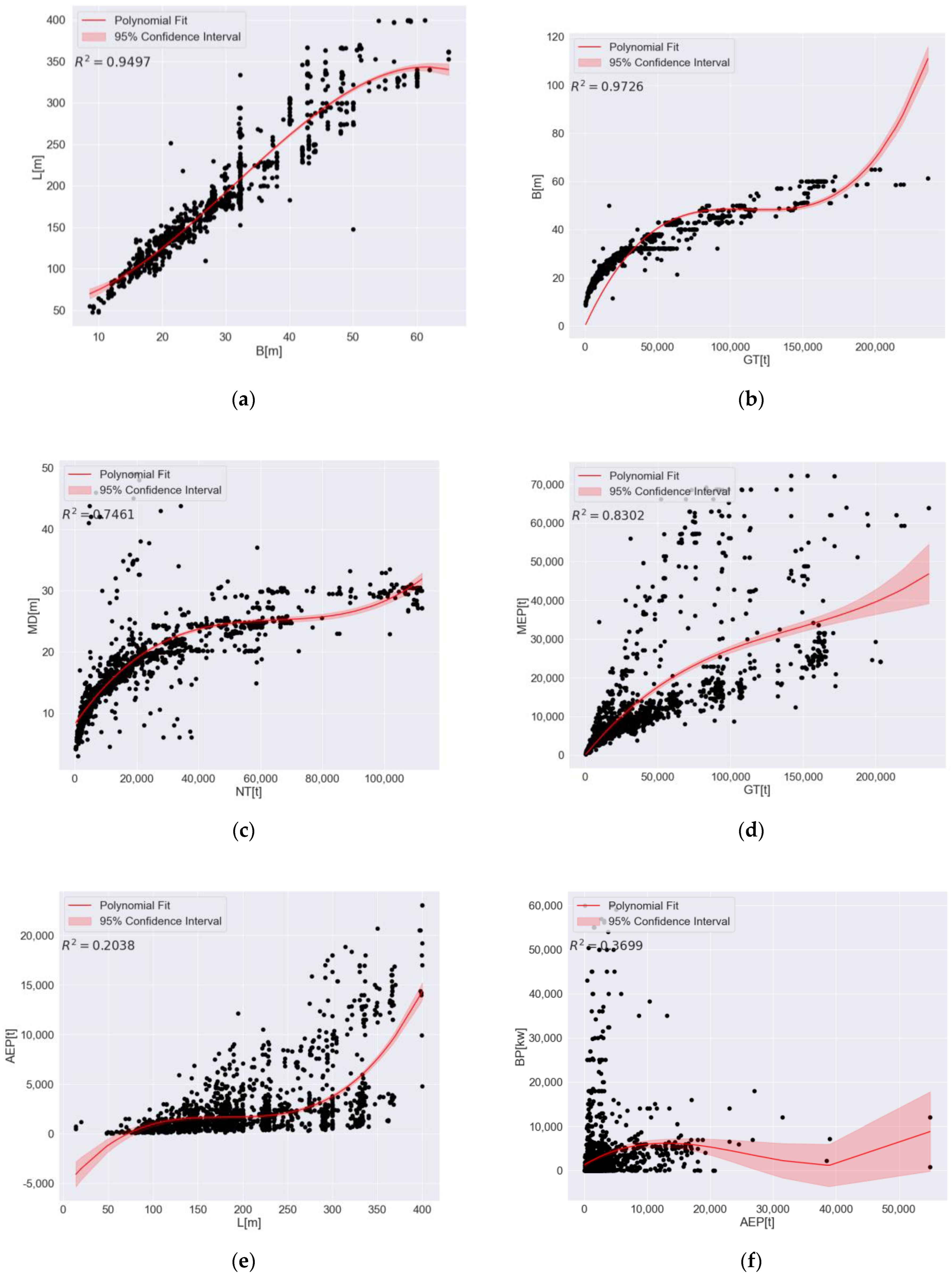
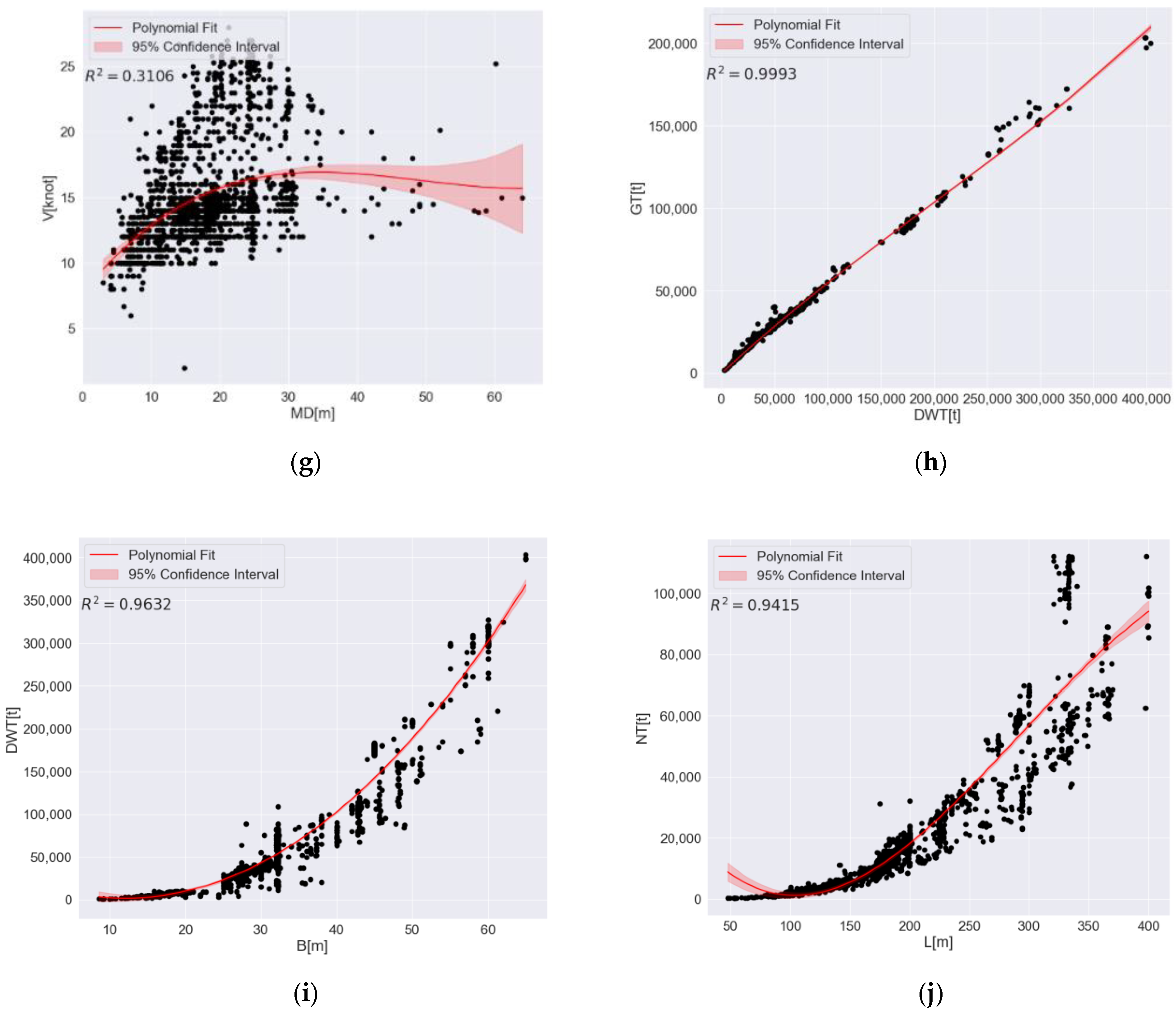
In the WFGAIN-GP model proposed in this study, the temporary filling values in the data preprocessing stage need to be obtained through the polynomial fitting. The function takes the parameter to be filled as y and the parameter with the highest R 2 value as x, and the determined function expression is y = k 0 + k 1 · x + k 2 · x   2 + k 3 · x   3 . The final fitting curve in this step is shown in Figure 5a–j, and the values of each coefficient are shown in Table 5. When the R 2 value is high, the fitting effect is good. As shown in Figure 5h, the R 2 value of GT and DWT is 0.9993, and their polynomial fitting functions are close to a straight line. As shown in Figure 5a,b,i, most of the parameters have high R 2 values and good fitting effects. The R 2 value of L and AEP is only 0.2038, indicating a weak correlation and poor fitting effect, as shown in Figure 5e. The R 2 value of BP and V are also low, and the corresponding fitting effects are poor, as shown in Figure 5f,g. For most parameters with poor fitting effects, it is difficult to ensure the accuracy of the data if the fitted data are directly used as the imputation value.
The temporary filling values obtained by polynomial fitting on this part of the fitted data are only used to replace the noisy data in GAIN and will not be directly applied for missing data imputation. The main purpose of filling in missing values is to help the model learn more potential patterns and data distribution information and improve its generalization performance. In the proposed model, a mask vector is used to distinguish between the original data and the temporary filling values, which are then input into the generator G and discriminator D. The temporary filling values that are closer to the true values can slightly improve the original model, making it more suitable for the application of ship data.

3.3. Comparative Experimental Analysis

This study compared the proposed imputation model with several existing missing value imputation models, including the early missing forest (MF) model, the polynomial fitting (PF) model, and the recently proposed GAIN model. The MF model can handle large-scale and high-dimensional data. Its basic idea is to use a set of random forest models, each of which uses different random samples and features to predict missing values [38]. The polynomial fitting model can be used to analyze the nonlinear relationship between data, and it can fit the data highly and then perform polynomial imputation [39]. The polynomial fitting model used here and the polynomial coefficients were selected from the data provided in Table 5. These models are currently widely used in missing data imputation.
This section of the study compared and analyzed the four models using RMSE, MAPE, and AUROC, with the corresponding missing rates being the overall missing rate of the data. Table 6 and Figure 6a show the RMSE values of the different models at different missing rates. Among the four models, the two methods based on generative adversarial network models are better than MF and PF. As the missing rate increases, the RMSE of PF approaches exponential growth, while the proposed models and GAIN show more stable linear growth. The proposed models and GAIN have similar RMSE values, but the RMSE values of the proposed models are slightly lower than GAIN. In the comparison of MAPE values, the two methods based on generative adversarial network models are also better than MF and PF, as shown in Table 7 and Figure 6b. Comparing the cases of missing rates of 10% and 20%, the RMSE and MAPE changes in WFGAIN-GP and GAIN are small, indicating that generative adversarial models have good robustness at low missing rates. PF is limited by the selection of specific features, and its RMSE and MAPE values are higher than the other three models. Table 8 and Figure 6c show the AUROC analysis results of MF, GAIN, and WFGAIN-GP. As the missing rate increases, the AUROC values of each model decrease significantly, but at higher missing rates, the performances of WFGAIN-GP and GAIN are significantly better than MF. This is because more missing values lead to a reduction in the information contained in the observed data, and the quality of imputation becomes more important, and GAIN has been proven to provide better quality imputation [30].
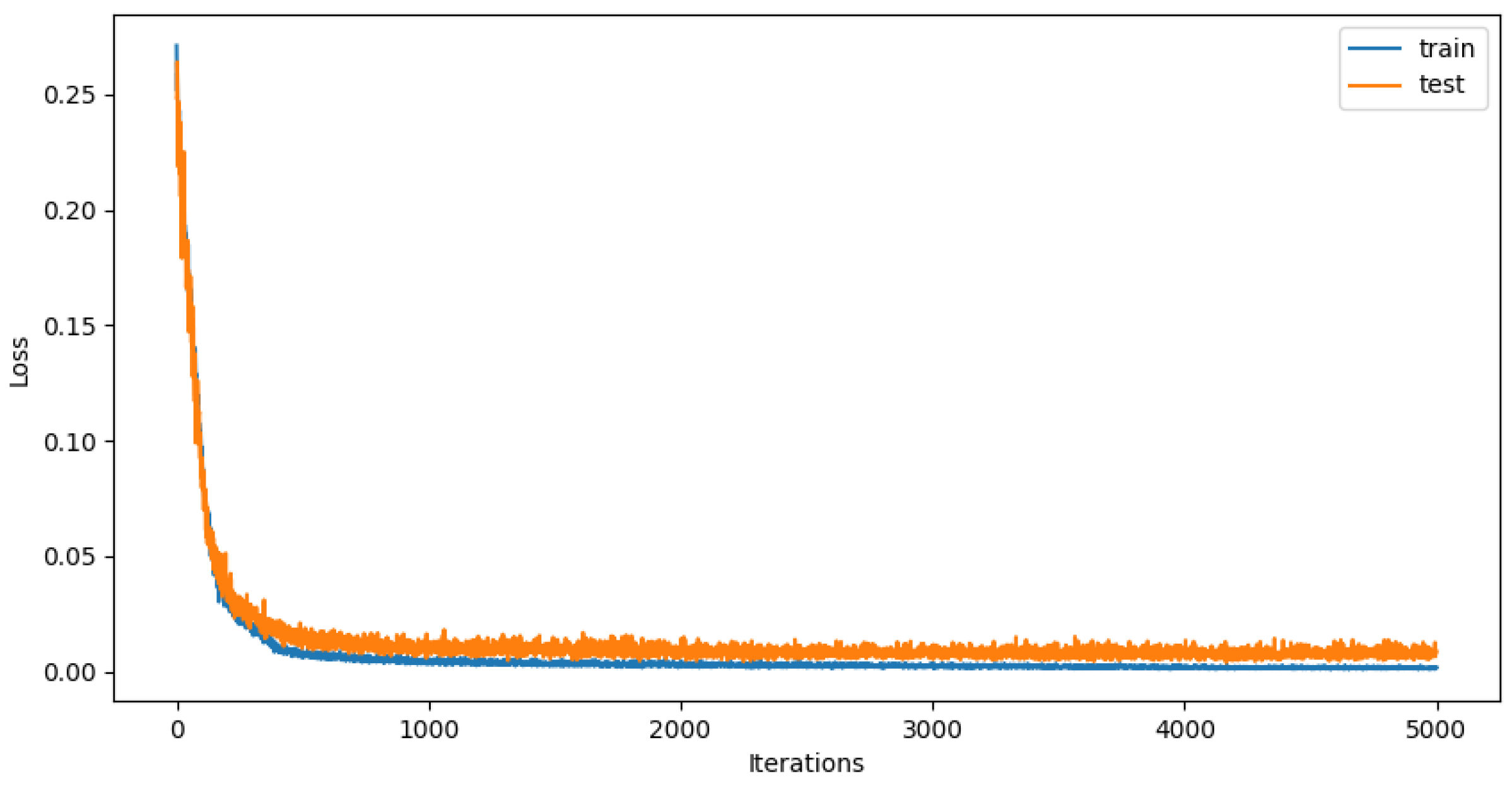
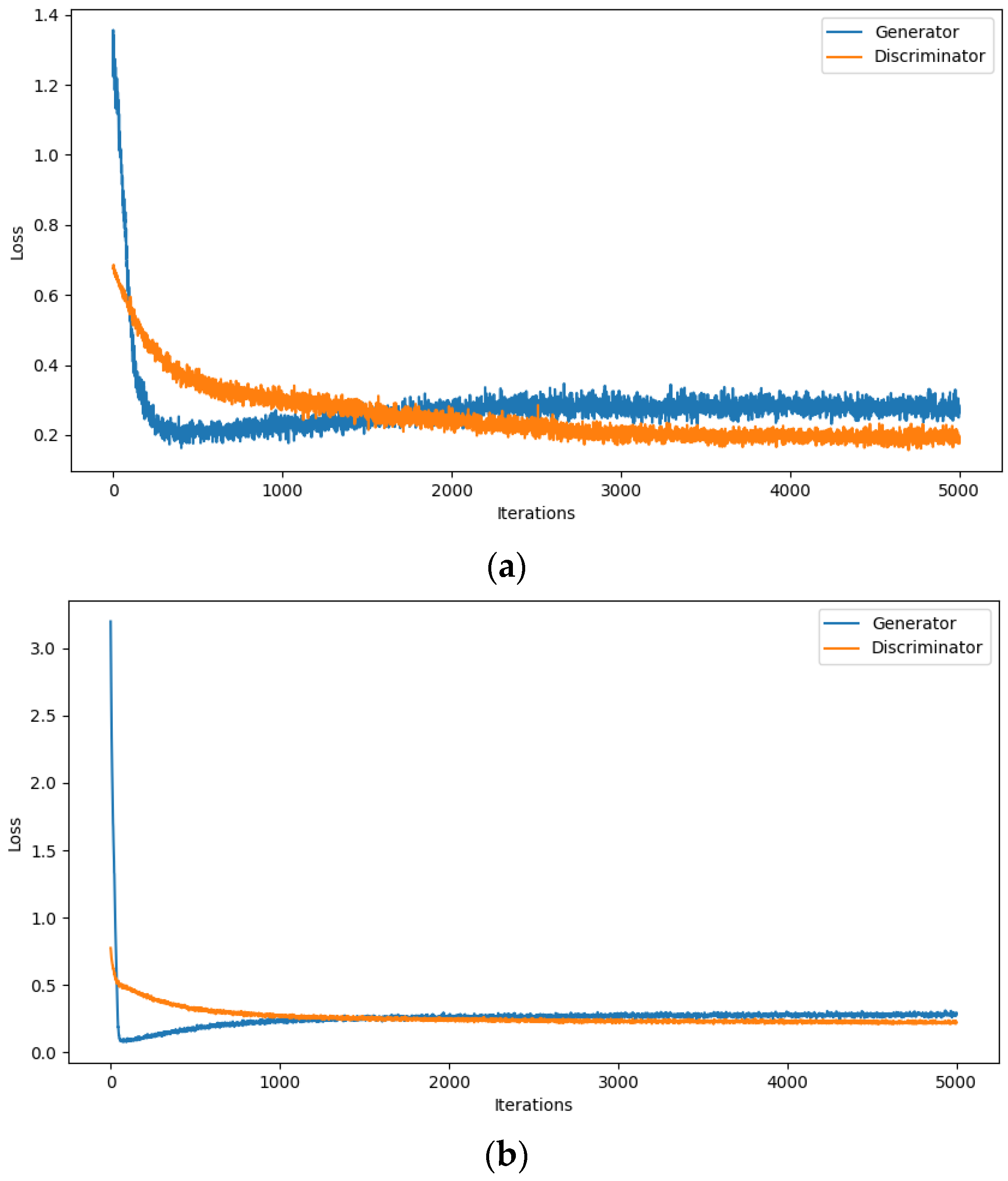
Figure 7 compares the accuracy of the WFGAIN-GP model on the training and testing sets with a 10% missing rate. With an increase in the number of iterations, the loss value significantly decreases and, after about 1000 iterations, there is no significant change, which also reflects the better generalization ability of the proposed model. Figure 8a,b show the iteration loss of the discriminator (D) and generator (G) during training for the GAIN and WFGAIN-GP models. It can be observed that both models have the common feature that the loss of the generator G quickly decreases to a small value, and then slightly increases and tends to stabilize. However, the difference is that during training, the oscillation of the loss of both D and G in the GAIN model is very large and unstable, while in the WFGAIN-GP model, the loss of D and G is relatively stable, and the changes in both lines are smoother as the iteration progresses. This also reflects the advantages of the Wasserstein distance and gradient penalty (GP).
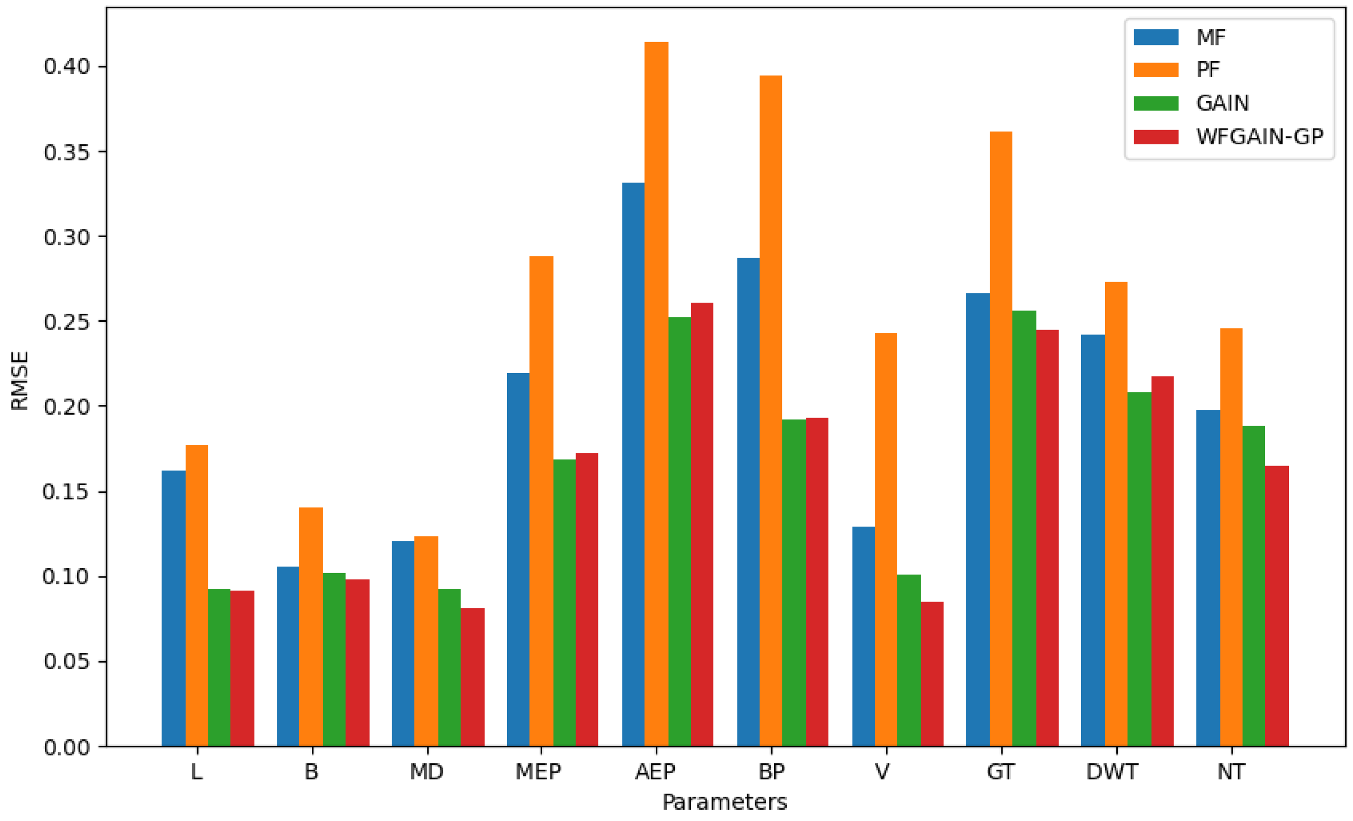
This study also analyzed the performance of the four models based on the actual missing distribution of the bulk carrier data and set the missing proportion of each design parameter accordingly. The actual missing rates of the 10 design parameters are shown in Table 9, and the actual missing distribution can more accurately test the practicality of the imputation models. Table 10 and Figure 9 analyze the RMSE values under the actual missing distribution, and the results show that the two methods based on the generative adversarial network model are better than MF and PF. The difference between WFGAIN-GP and GAIN is small, but in the comparison of RMSE values of six design parameters, namely L, B, MD, V, GT, and NT, WFGAIN-GP is slightly better than GAIN, as shown in the comparison in Figure 9. The results show that WFGAIN-GP also has good applicability to the actual missing distribution.

3.4. Analysis of Different Characteristic Dimensions

This study also discusses the case of different feature dimensions and analyzes the impact of the number of features on imputation performance. The impact of different feature dimensions on the model depends on several factors, including the model type, the size and dimensionality of the dataset, and the correlation and importance of the features themselves. A low feature dimensionality may result in information loss and prevent the model from capturing all critical features in the data. The importance of features can affect the choice and performance of the model. Some features may be more important than others and, therefore, should be prioritized in the imputation process. In this study, features with higher R 2 values were given priority.
Table 11 and Figure 10a,b present the analysis of V and MEP in the reference dataset, considering the number of reference features ranging from two to nine. In this experiment, the missing data rate follows the real distribution proportions given in Table 9. As the feature dimensionality decreases, the RMSE values of WFGAIN-GP and GAIN show less variation, while the RMSE value of MF increases significantly. This indicates that the two methods based on generative adversarial network models are robust to the number of feature dimensions. When the number of feature dimensions is small, the discriminative model MF is not very good at handling such data. Generative adversarial models can generate new data based on the overall data, without relying on a specific feature, so the impact of dimensionality on such models is lower than on discriminative models.

3.5. Imputation of Real Missing Values

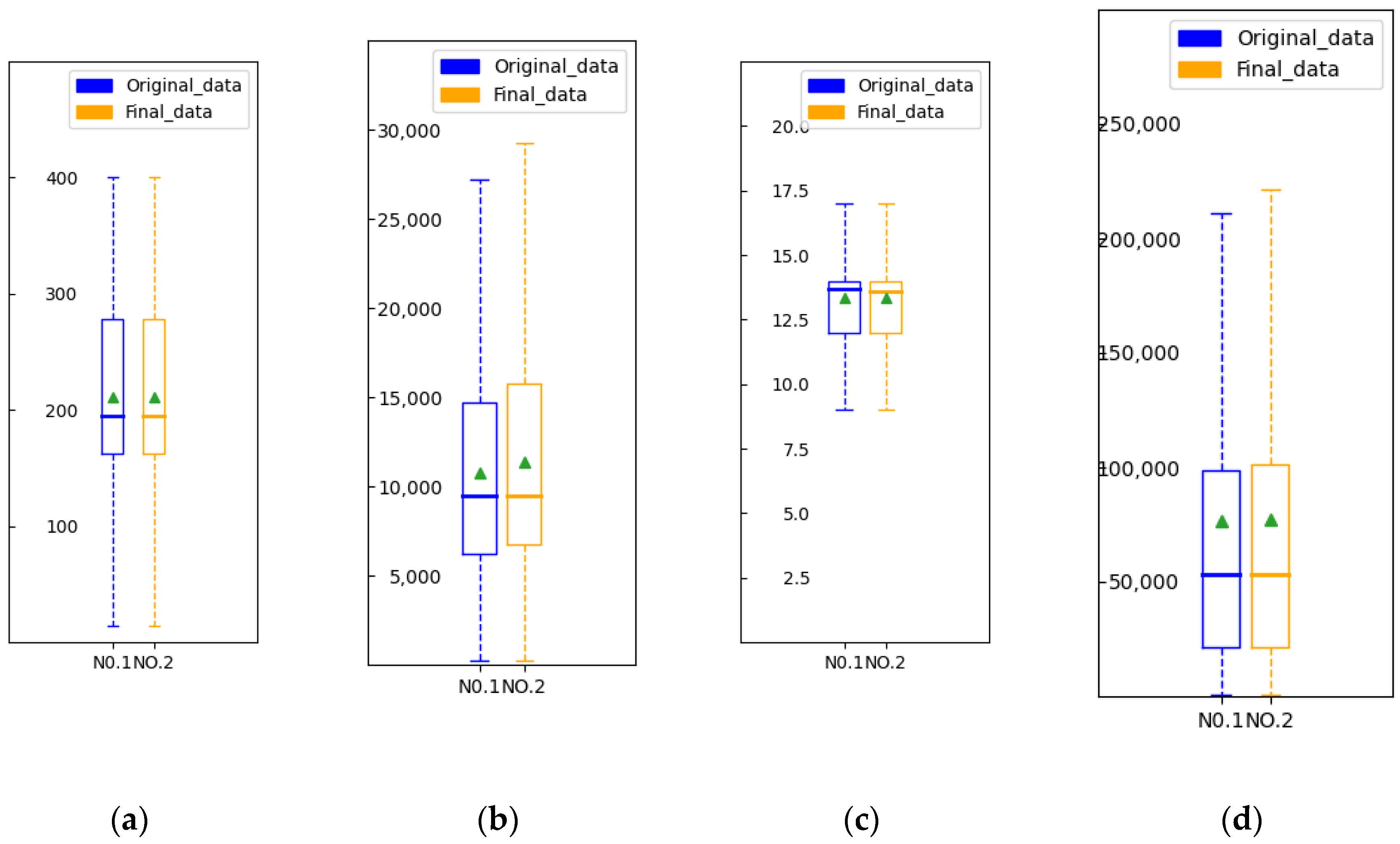
In the above experimental analysis, the WFGAIN-GP model demonstrated good performance in all performance comparisons. In this section, this model will be used to handle real missing data problems. Four design parameters with different missing rates are selected for imputation analysis, including the two design parameters AEP and V with the highest missing rate, and the two design parameters L and NT with lower missing rates. As shown in the box plots in Figure 11a–d, the minimum value, maximum value, mean value, lower quartile (25%), and upper quartile (75%) of L and V almost remain unchanged. In the case of AEP and NT, the values of the lower and upper quartiles have slightly changed, but the changes are small, and the mean value almost remains unchanged. This indicates that the missing rate has a small impact on the performance of the proposed model, and the inherent properties of the features to be predicted may be the main factors affecting the prediction accuracy.
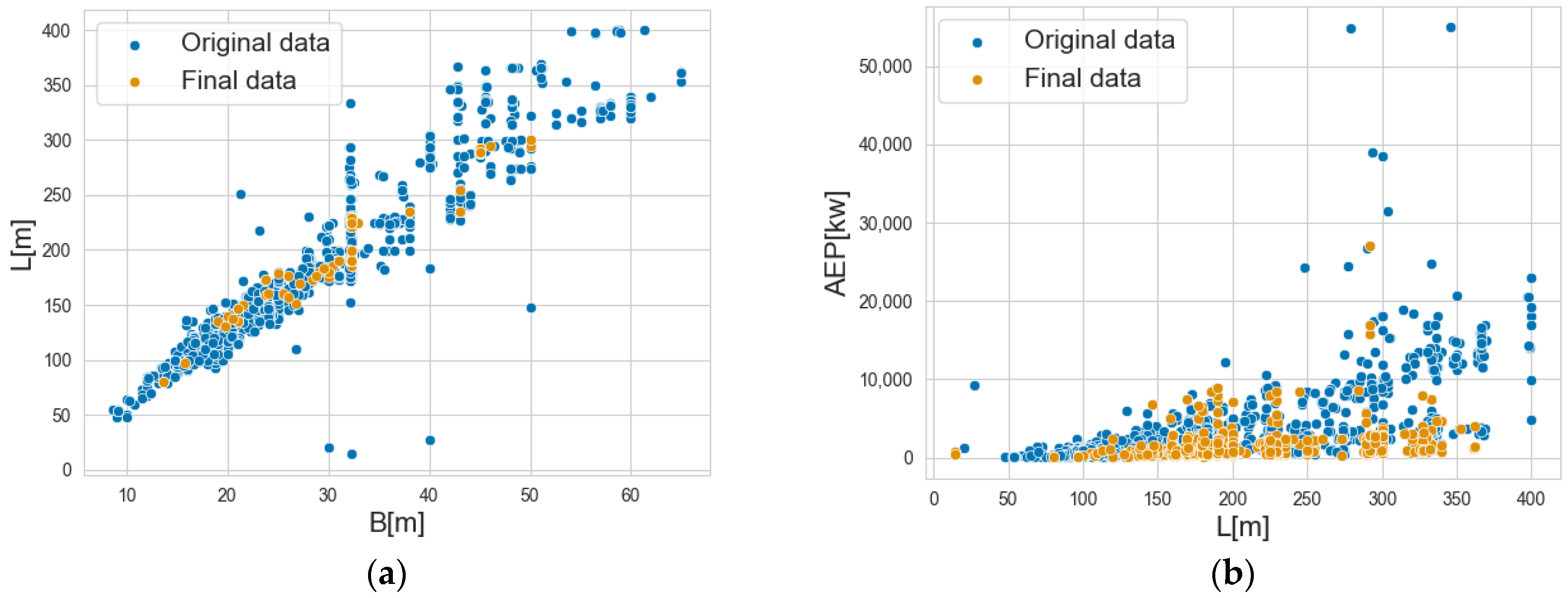
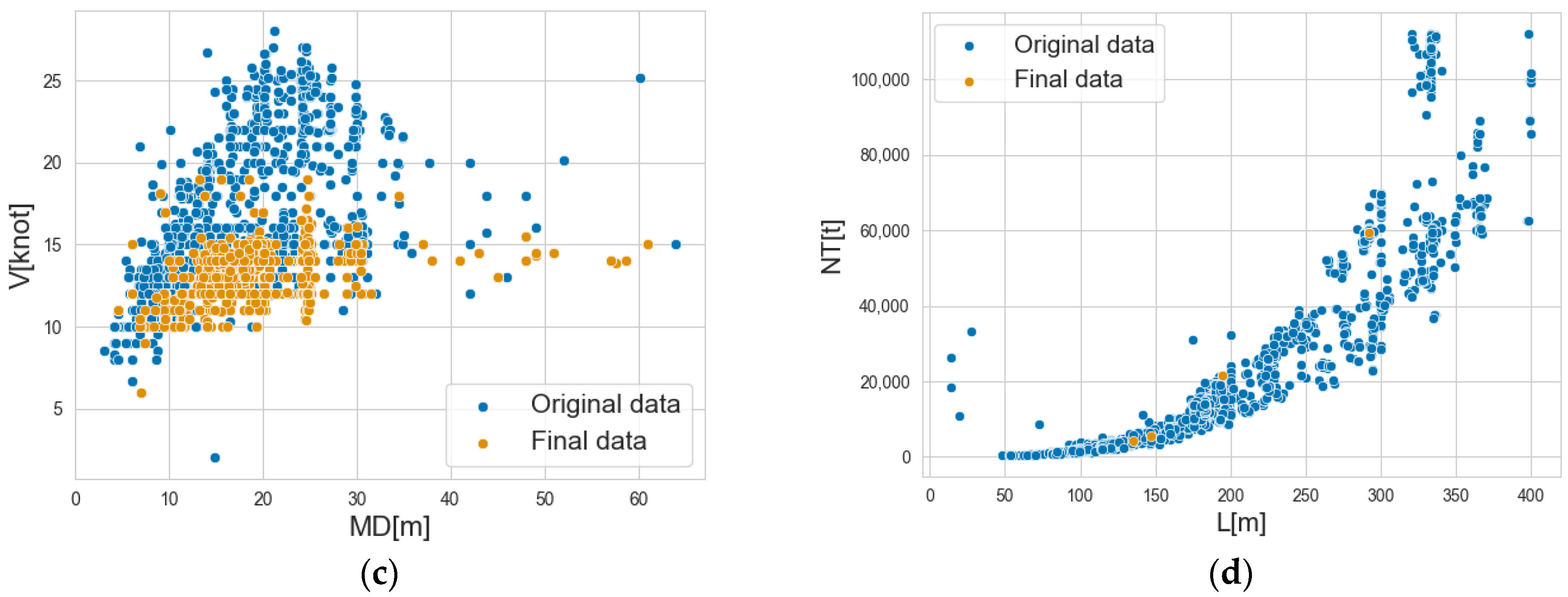
A comparison between the predicted and original data can be seen in Figure 12, which displays scatter plots of the parameters that require imputation and those with the highest R 2 values. There is good consistency between the predicted data and the original data, whether it is the AEP and V parameters with high missing rates or the L and NT parameters with low missing rates. In Figure 12b,c, the predicted data distribution is more scattered, and most data points do not lie on the polynomial fitting curve (see Figure 5e,g). This is because the goals of generative adversarial networks and regression fitting are different. The former generates data through adversarial training and autonomously learns the distribution characteristics of the data, while the latter predicts data through a given function form and is constrained by specific features. Based on the experimental analysis in Section 3.4, the predicted data does not deviate significantly from the statistical features of the original data, indicating that the proposed model has good applicability for imputing missing ship data.

4. Conclusions

This study proposed a missing data imputation method based on generative adversarial networks (GANs) and validated it using 10 design parameters of 8167 bulk carrier ships, demonstrating that the proposed model performs well and can be widely applied to missing data processing in static ship data. The proposed model is an improvement of the generative adversarial imputation network (GAIN) and has three main modifications. First, it uses polynomial fitting values closer to the true values instead of random noise as temporary fill values, making it easier for the model to learn the feature distribution of ship data. Second, it introduces Wasserstein distance instead of Jensen–Shannon divergence (JSD) to measure the distance between the generated data distribution and the real data distribution, which can avoid the mode collapse problem in GAN and increase the robustness of the model. Third, gradient penalty (GP) is added to further improve the model’s stability by addressing gradient vanishing or explosion issues. In the data preprocessing stage, this study also proposed combining ship domain knowledge and the isolation forest (IF) to detect outliers in the original data. For the predicted values output by the proposed model, it is necessary to check whether they are within the normal range and correct abnormal predicted values.
This study also conducted statistical analysis on ship data, including correlation analysis of ship design parameters, outlier analysis, and analysis of missing data types. These analyses provided the basis for the proposed imputation method. To validate the model’s performance, the proposed WFGAIN-GP model was compared with the missing forest (MF), polynomial fitting (PF), and generative adversarial imputation nets (GAIN) in a comparative experiment. Based on multiple validation standards, such as RMSE, MAPE, and AUROC, the WFGAIN-GP model outperformed the MF and PF models and was also more stable than the GAIN model. The proposed model also performed well in comparative experiments with different feature dimensions. Therefore, it can be concluded that the proposed method is suitable for imputing missing values in ship static data.
Future research will examine the effectiveness of this imputation method applied to different ship datasets and will further improve the method proposed in this study through validation on different datasets. Current static data imputation methods mainly focus on the quality of the interpolated data. Future research can consider uncertainty estimation methods to evaluate the confidence and reliability of the imputed data, providing a more accurate basis for subsequent data processing and analysis. In addition, the interpretability of deep learning models is also a key focus.

Author Contributions

J.G.: conceptualization, software, design, analysis, writing—original draft, and reviews; Z.C.: conceptualization, structural calculations, analysis, writing—original draft, and reviews; W.S.: conceptualization, validation, analysis, and writing—original draft; Y.J.: conceptualization, validation, analysis, and writing—original draft. All authors have read and agreed to the published version of the manuscript.

Funding

This work was supported by the Innovation Program of the Shanghai Municipal Education Commission (grant no. 2021-01-07-00-10-E00121).

Institutional Review Board Statement

Not applicable.

Informed Consent Statement

Not applicable.

Data Availability Statement

Not applicable.

Acknowledgments

The authors would like to thank the Innovation Program of the Shanghai Municipal Education Commission (grant no. 2021-01-07-00-10-E00121) for its support. The authors also acknowledge the anonymous reviewers for their suggestions that improved the manuscript.

Conflicts of Interest

The authors declare no conflict of interest.

Appendix A

Descriptive statistics of main design parameters of other types of ships:
Table A1. Descriptive statistics of the main design parameters of 3142 container ships in ship static data.
Ship Principal ParametersValid DataMissing DataMeanMedianMinimumMaximumStd. DevSkewnessKurtosis
L [m]309052255.3400.0263.250.083.8−0.14−1.06
B [m]295019236.161.532.311.310.60.22−0.70
MD [m]243470818.829.919.14.05.9−0.02−0.77
MEP [kw]284429837,619.9122,650.036,560.0933.024,093.10.33−0.81
AEP [kw]197211706436.388,180.04000.080.06700.63.2525.24
BP [kw]25955472585.67000.02000.07.52056.00.42−1.16
V [knot]1673146920.928.822.05.04.0−1.091.08
GT [t]3142064,360.0236,583.047,914.0967.053,233.81.020.41
DWT [t]31291370,955.8658,129.058,255.01.054,083.51.174.11
NT [t]3141133,180.7130,371.024,504.0468.027,406.60.900.13
Table A2. Descriptive statistics of the main design parameters of 4991 tankers in ship static data.
Ship Principal ParametersValid DataMissing DataMeanMedianMinimumMaximumStd. DevSkewnessKurtosis
L [m]495446211.722840.834091.1−0.17−1.2
B [m]473925236.132.3760.117.4−0.01−1.32
MD [m]428970216.218.8329.88.1−0.05−1.29
MEP [kw]454244914,727.812,50080062,7499597.40.650.28
AEP [kw]366313281768.611106033,3512333.86.1759.04
BP [kw]301919721426.27201071001637.81.30.93
V [knot]3694129713.6146482.42.4339
GT [t]4987463,034.342,884424170,61159,140.40.71−0.97
DWT [t]49838116,425.674,993498380,000114,894.90.77−0.93
NT [t]4990138,544.422,259.560112,28139,900.40.85−0.85
Table A3. Little’s MCAR test.
Static Database (Container Ship)Static Database (Oil Tanker)
χ 2 V a l u e d f p V a l u e χ 2 V a l u e d f p V a l u e
205.440910.000514.4171310.000

Appendix B

Predictive analysis of the main design parameters of other types of ships:
Table A4. RMSE values of imputation results of each model for container ship and tanker data with different missing rates.
AlgorithmRMSE
Container ShipOil Tanker
10%20%30%40%50%60%10%20%30%40%50%60%
MF0.2250.2320.2410.2490.2680.2910.2540.2680.2880.2970.3290.344
PF0.2730.2830.3120.3370.3420.3590.2890.3070.3230.3470.3560.381
GAIN0.2150.2210.2350.2460.2580.2690.2320.2420.2490.2550.2630.270
WFGAIN-GP0.2160.2190.2380.2430.2550.2730.2410.2430.2510.2620.2670.275
Table A5. The RMSE values of imputation based on the actual missing rate for container ship and oil tanker data.
RMSE
Ship Principal ParametersContainer ShipOil Tanker
MFPFGAINWFGAIN-GPMFPFGAINWFGAIN-GP
L [m]0.1660.1850.9890.1090.1750.2270.1050.101
B [m]0.1350.1940.1090.1170.1560.2350.1280.108
MD [m]0.1970.2010.1150.1030.1990.2160.1190.115
MEP [kw]0.2110.3360.1780.1880.2300.3560.2040.196
AEP [kw]0.3470.4500.2960.2930.3580.4830.2780.281
BP [kw]0.3120.4430.2550.2340.3270.4550.2510.245
V [knot]0.1750.2250.1430.1310.1330.1630.1030.106
GT [t]0.3230.4170.2690.2780.3370.4540.2910.289
DWT [t]0.2960.3630.2680.2500.3190.4080.2630.267
NT [t]0.2440.2980.2070.1920.2660.3690.1970.189

References

  1. Sirimanne, S.N.; Hoffman, J.; Juan, W.; Asariotis, R.; Assaf, M.; Ayala, G.; Benamara, H.; Chantrel, D.; Hoffmann, J. Review of maritime transport 2019. In Proceedings of the United Nations Conference on Trade and Development, Geneva, Switzerland, 24–25 September 2019. [Google Scholar]
  2. Imtiaz, S.A.; Shah, S.L. Treatment of missing values in process data analysis. Can. J. Chem. Eng. 2008, 86, 838–858. [Google Scholar] [CrossRef]
  3. Khatibisepehr, S.; Huang, B.; Khare, S. Design of inferential sensors in the process industry: A review of Bayesian methods. J. Process Control 2013, 23, 1575–1596. [Google Scholar] [CrossRef]
  4. Wang, Z.; Claramunt, C.; Wang, Y. Extracting global shipping networks from massive historical automatic identification system sensor data: A bottom-up approach. Sensors 2019, 19, 3363. [Google Scholar] [CrossRef] [PubMed] [Green Version]
  5. Jaskólski, K.; Marchel, Ł.; Felski, A.; Jaskólski, M.; Specht, M. Automatic Identification System (AIS) Dynamic Data Integrity Monitoring and Trajectory Tracking Based on the Simultaneous Localization and Mapping (SLAM) Process Model. Sensors 2021, 21, 8430. [Google Scholar] [CrossRef] [PubMed]
  6. Liu, C.; Chen, X. Inference of single vessel behaviour with incomplete satellite-based AIS data. J. Navig. 2013, 66, 813–823. [Google Scholar] [CrossRef] [Green Version]
  7. Mao, S.; Tu, E.; Zhang, G.; Rachmawati, L.; Rajabally, E.; Huang, G.B. An automatic identification system (AIS) database for maritime trajectory prediction and data mining. In Proceedings of the ELM-2016, Singapore, 13–15 December 2016; Springer International Publishing: Cham, Switzerland, 2018; pp. 241–257. [Google Scholar]
  8. Dobrkovic, A.; Iacob, M.E.; van Hillegersberg, J. Maritime pattern extraction and route reconstruction from incomplete AIS data. Int. J. Data Sci. Anal. 2018, 5, 111–136. [Google Scholar] [CrossRef] [Green Version]
  9. Gutierrez-Torre, A.; Berral, J.L.; Buchaca, D.; Guevara, M.; Soret, A.; Carrera, D. Improving maritime traffic emission estimations on missing data with CRBMs. Eng. Appl. Artif. Intell. 2020, 94, 103793. [Google Scholar] [CrossRef]
  10. Guo, S.; Mou, J.; Chen, L.; Chen, P. Improved kinematic interpolation for AIS trajectory reconstruction. Ocean Eng. 2021, 234, 109256. [Google Scholar] [CrossRef]
  11. Gao, D.W.; Zhu, Y.S.; Zhang, J.F.; He, Y.K.; Yan, K.; Yan, B.R. A novel MP-LSTM method for ship trajectory prediction based on AIS data. Ocean Eng. 2021, 228, 108956. [Google Scholar] [CrossRef]
  12. Cheliotis, M.; Gkerekos, C.; Lazakis, I.; Theotokatos, G. A novel data condition and performance hybrid imputation method for energy efficient operations of marine systems. Ocean Eng. 2019, 188, 106220. [Google Scholar] [CrossRef]
  13. Gao, J.; Cai, Z.; Yu, W.; Sun, W. Trajectory Data Compression Algorithm Based on Ship Navigation State and Acceleration Variation. J. Mar. Sci. Eng. 2023, 11, 216. [Google Scholar] [CrossRef]
  14. Ekinci, S.; Çelebi, U.B.; Bal, M.; Amasyali, M.F.; Boyaci, U.K. Predictions of oil/chemical tanker main design parameters using computational intelligence techniques. Appl. Soft Comput. 2011, 11, 2356–2366. [Google Scholar] [CrossRef]
  15. Chen, D.; Wang, X.; Li, Y.; Lang, J.; Zhou, Y.; Guo, X.; Zhao, Y. High-spatiotemporal-resolution ship emission inventory of China based on AIS data in 2014. Sci. Total Environ. 2017, 609, 776–787. [Google Scholar] [CrossRef] [PubMed]
  16. Huang, L.; Wen, Y.; Zhang, Y.; Zhou, C.; Zhang, F.; Yang, T. Dynamic calculation of ship exhaust emissions based on real-time AIS data. Transp. Res. Part D Transp. Environ. 2020, 80, 102277. [Google Scholar] [CrossRef]
  17. Abramowski, T.; Cepowski, T.; Zvolenský, P. Determination of regression formulas for key design characteristics of container ships at preliminary design stage. New Trends Prod. Eng. 2018, 1, 247–257. [Google Scholar] [CrossRef] [Green Version]
  18. Gurgen, S.; Altin, I.; Ozkok, M. Prediction of main particulars of a chemical tanker at preliminary ship design using artificial neural network. Ships Offshore Struct. 2018, 13, 459–465. [Google Scholar] [CrossRef]
  19. Kim, Y.; Steen, S.; Muri, H. A novel method for estimating missing values in ship principal data. Ocean Eng. 2022, 251, 110979. [Google Scholar] [CrossRef]
  20. Goodfellow, I.J.; Pouget-Abadie, J.; Mirza, M.; Xu, B.; Warde-Farley, D.; Ozair, S.; Courville, A.; Bengio, Y. Generative Adversarial Networks. arXiv 2014, arXiv:1406.2661. [Google Scholar] [CrossRef]
  21. Arjovsky, M.; Bottou, L. Towards principled methods for training generative adversarial networks. arXiv 2017, arXiv:1701.04862. [Google Scholar]
  22. Arjovsky, M.; Chintala, S.; Bottou, L. Wasserstein generative adversarial networks. In Proceedings of the International Conference on Machine Learning, PMLR, Honolulu, HI, USA, 23–29 July 2017; pp. 214–223. [Google Scholar]
  23. Sun, J.; Bhattarai, B.; Chen, Z.; Kim, T.K. Secgan: Parallel conditional generative adversarial networks for face editing via semantic consistency. arXiv 2021, arXiv:2111.09298. [Google Scholar]
  24. Pei, H.; Ren, K.; Yang, Y.; Liu, C.; Qin, T.; Li, D. Towards generating real-world time series data. In Proceedings of the 2021 IEEE International Conference on Data Mining (ICDM), Auckland, New Zealand, 7–10 December 2021; IEEE: New York, NY, USA, 2021; pp. 469–478. [Google Scholar]
  25. Shi, Y.; Han, L.; Han, L.; Chang, S.; Hu, T.; Dancey, D. A latent encoder coupled generative adversarial network (le-gan) for efficient hyperspectral image super-resolution. IEEE Trans. Geosci. Remote Sens. 2022, 60, 3193441. [Google Scholar] [CrossRef]
  26. Poudevigne-Durance, T.; Jones, O.D.; Qin, Y. MaWGAN: A generative adversarial network to create synthetic data from datasets with missing data. Electronics 2022, 11, 837. [Google Scholar] [CrossRef]
  27. Nadimi-Shahraki, M.H.; Mohammadi, S.; Zamani, H.; Gandomi, M.; Gandomi, A.H. A hybrid imputation method for multi-pattern missing data: A case study on type II diabetes diagnosis. Electronics 2021, 10, 3167. [Google Scholar] [CrossRef]
  28. Gulrajani, I.; Ahmed, F.; Arjovsky, M.; Dumoulin, V.; Courville, A.C. Improved training of wasserstein gans. In Advances in Neural Information Processing Systems; MIT: Cambridge, MA, USA, 2017; Volume 30. [Google Scholar]
  29. Radford, A.; Metz, L.; Chintala, S. Unsupervised representation learning with deep convolutional generative adversarial networks. arXiv 2015, arXiv:1511.06434. [Google Scholar]
  30. Yoon, J.; Jordon, J.; Schaar, M. Gain: Missing data imputation using generative adversarial nets. In Proceedings of the International Conference on Machine Learning, PMLR, Stockholm, Sweden, 10–15 July 2018; pp. 5689–5698. [Google Scholar]
  31. Wang, Y.; Li, D.; Li, X.; Yang, M. PC-GAIN: Pseudo-label conditional generative adversarial imputation networks for incomplete data. Neural Netw. 2021, 141, 395–403. [Google Scholar] [CrossRef]
  32. Neves, D.T.; Alves, J.; Naik, M.G.; Proenca, A.J.; Prasser, F. From missing data imputation to data generation. J. Comput. Sci. 2022, 61, 101640. [Google Scholar] [CrossRef]
  33. Dong, W.; Fong, D.; Yoon, J.; Wan, E.; Bedford, L.; Tang, E.; Lam, C. Generative adversarial networks for imputing missing data for big data clinical research. BMC Med. Res. Methodol. 2021, 21, 78. [Google Scholar] [CrossRef]
  34. Zhang, W.; Zhang, P.; Yu, Y.; Li, X.; Biancardo, S.A.; Zhang, J. Missing data repairs for traffic flow with self-attention generative adversarial imputation net. IEEE Trans. Intell. Transp. Syst. 2021, 23, 7919–7930. [Google Scholar] [CrossRef]
  35. International Maritime Organization (IMO). Fourth Greenhouse Gas Study. 2020. Available online: https://www.imo.org/en/OurWork/Environment/Pages/Fourth-IMO-Greenhouse-Gas-Study-2020.aspx (accessed on 16 January 2023).
  36. Rubin, D.B. Inference and missing data. Biometrika 1976, 63, 581–592. [Google Scholar] [CrossRef]
  37. Little, R.J. A test of missing completely at random for multivariate data with missing values. J. Am. Stat. Assoc. 1988, 83, 1198–1202. [Google Scholar] [CrossRef]
  38. Breiman, L. Random forests. Mach. Learn. 2001, 45, 5–32. [Google Scholar] [CrossRef] [Green Version]
  39. Tong, Y.; Yu, L.; Li, S.; Liu, J.; Qin, H.; Li, W. Polynomial fitting algorithm based on neural network. ASP Trans. Pattern Recognit. Intell. Syst. 2021, 1, 32–39. [Google Scholar] [CrossRef]
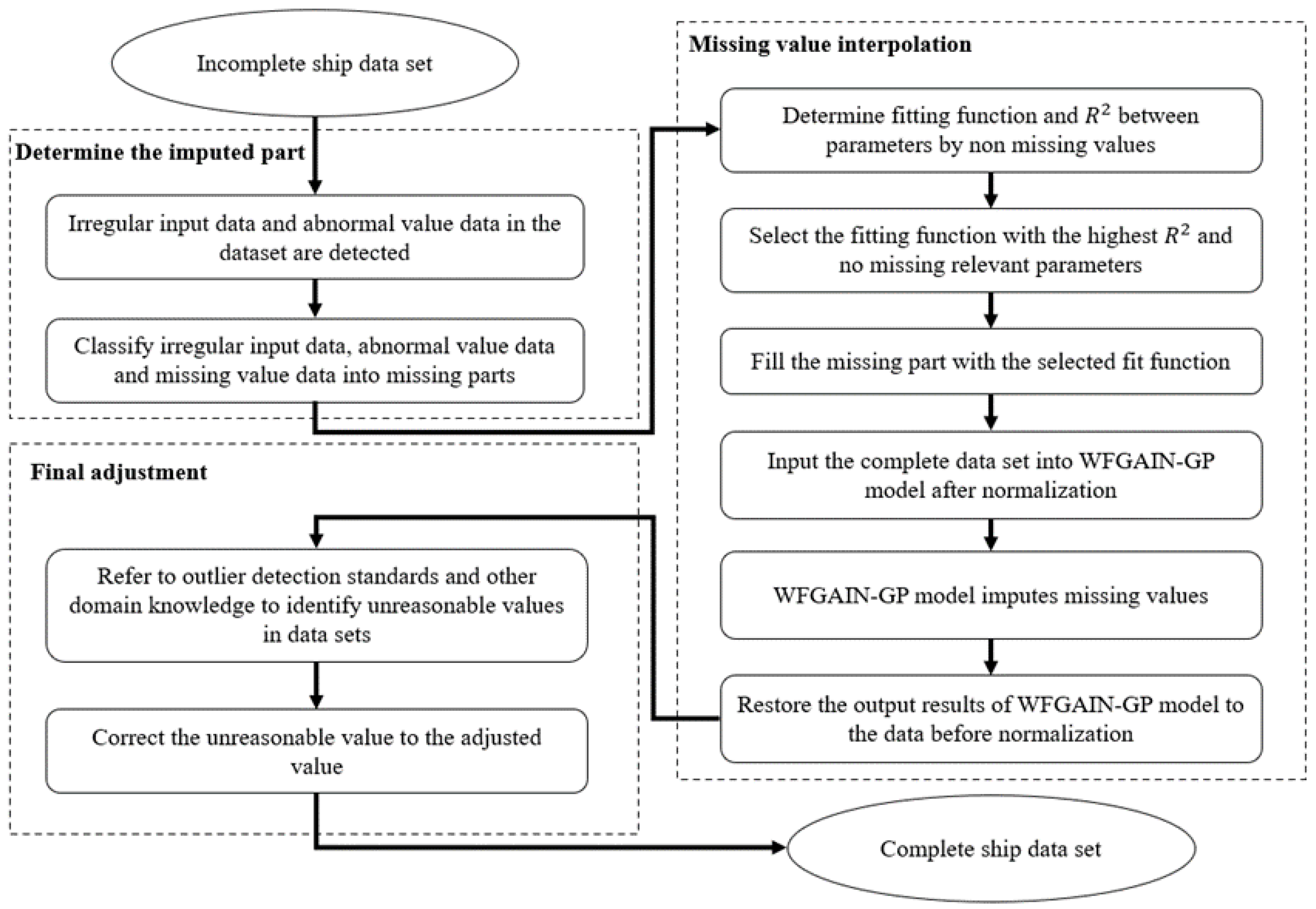
Figure 1. Flowchart for imputing missing values in static ship data. Firstly, identify the part of the data that needs to be imputed, then use the WFGAIN-GP model to impute this part of the data, and finally fine-tune it through experience in the relevant field.
Jmse 11 00806 g001
Figure 2. The framework of WFGAIN-GP. The temporarily padded data, original data, and mask are input into the generator together. Under the constraint of gradient penalty, the generator outputs the imputed complete data. The discriminator D receives the masked data processed by the hint mechanism and the complete data generated by the generator G and then outputs the discrimination result, which is a new mask.
Jmse 11 00806 g002
Figure 3. Analysis of R 2 values of the goodness of fit between each design parameter. The correlation coefficient “R” can measure the correlation between two variables, with a correlation close to 1 indicating a strong positive correlation between variables, close to −1 indicating a strong negative correlation between variables, and close to 0 indicating a slight relationship between variables. The R 2 value is used to measure the fitting degree of linear regression.
Jmse 11 00806 g003
Figure 4. Box plots of descriptive statistics for raw data: L, MEP, GT, and DWT. The green triangle represents the mean value, and the hollow circles represent the outliers.
Jmse 11 00806 g004
Figure 5. Polynomial fitting results for the main design parameters of the ship: (a) L, (b) B, (c) MD, (d) MEP, (e) AEP, (f) BP, (g) V, (h) GT, (i) DWT, and (j) NT. The black dots are the pre-processed data.
Jmse 11 00806 g005aJmse 11 00806 g005b
Figure 6. Performance comparison of different models under different missing rates: (a) RMSE, (b) MAPE, and (c) AUROC.
Jmse 11 00806 g006
Figure 7. Training and testing iteration loss information.
Jmse 11 00806 g007
Figure 8. The iteration loss of the generator D and discriminator G: (a) GAIN, and (b) WFGAIN-GP.
Jmse 11 00806 g008
Figure 9. Bar chart comparing the four imputation models under real missing rates.
Jmse 11 00806 g009
Figure 10. RMSE analysis plots for three models with a different number of features: (a) V and (b) MEP.
Jmse 11 00806 g010
Figure 11. Boxplots of descriptive statistics for the original data (blue box) and final data (orange box): (a) L, (b) AEP, (c) V, and (d) NT. The green triangle represents the mean value.
Jmse 11 00806 g011
Figure 12. Comparison between the original data (blue dots) and final data (orange dots): (a) L, (b) AEP, (c) V, and (d) NT.
Jmse 11 00806 g012aJmse 11 00806 g012b
Table 1. The range of values for detecting outliers of the ship-related design parameters includes 10 design parameters, namely length (L), breadth (B), molded depth (MD), main engine power (MEP), auxiliary engine power (AEP), boiler power (BP), rated speed (V), gross tonnage (GT), deadweight tonnage (DWT), and net tonnage (NT).
Attribute Column NameThe Upper Limit of the RangeThe Lower Limit of the Range
L [m]5001
B [m]801
MD [m]501
MEP [kw]150,000750
AEP [kw]100,00060
BP [kw]72007.2
V [knot]505
GT [t]1,000,000400
DWT [t]800,0001
NT [t]1,000,000 and ≤GT1
Table 2. Descriptive statistics of the main design parameters of 8167 bulk carriers in ship static data.
Ship Principal ParametersValid DataMissing DataMeanMedianMinimumMaximumStd. DevSkewnessKurtosis
L [m]808582211.0199.932.3362.054.70.240.08
B [m]766050733.632.38.865.09.000.621.05
MD [m]6948121918.118.32.729.94.73−0.320.11
MEP [kw]778538210,228.49070.0750100,000.05844.203.8440.80
AEP [kw]512830391322.6920.075.027,000.01342.226.5279.83
BP [kw]687112961011.7885.07.27200.0985.972.308.91
V [knot]5050311713.113.06.024.01.450.162.49
GT [t]8160744,836.534,773.0436371,06634,037.111.784.44
DWT [t]81402782,416.561,003.51.0766,044.068,444.741.905.56
NT [t]8163425,923.720,020.0101216,49618,567.551.151.38
Table 3. Statistical analysis of the missing proportion of the main design parameters for 8167 bulk carriers.
Number of Missing Parameters012345678910
Number of ships33481333325282151100000
Percentage40.99%16.32%39.82%1.00%1.85%0.01%0.00%0.00%0.00%0.00%0.00%
Table 4. Little’s MCAR test for the ship static data was used in the study. The test is based on comparing the observed pattern of missing data to what would be expected if the data were missing completely at random. If the test fails to reject the null hypothesis that the data are missing completely at random, then it can be assumed that the missing data do not depend on any unobserved variables and can be safely ignored in subsequent analyses. The χ 2 v a l u e is a test statistic used to compare the fit between observed and theoretical values. Degrees of freedom ( d f ) are used to calculate the number of independent variables in a statistical test. The p v a l u e is the result of a hypothesis test and represents the probability that the data fit the MCAR assumption. If the p v a l u e is less than the significance level (usually 0.05), then the MCAR assumption can be rejected.
χ 2 V a l u e d f p V a l u e
Static database
(Bulk cargo ship)
1075.6462180.000
Table 5. The coefficients of the polynomial fit function. Functional expression: y = k 0 + k 1 · x + k 2 · x   2 + k 3 · x   3 .
ParameterCoefficient of the Polynomial Function
yx k 0 k 1 k 2 k 3
LB 5.83979739 × 10 1 4.54031032 × 10 1 2.40225732 × 10 1 2.56007337 × 10 3
BGT 6.13880921 × 10 8 1.31028580 × 10 3 1.16999326 × 10 8 3.44233924 × 10 14
MDNT 8.41699396 × 10 0 7.10232369 × 10 4 1.01075453 × 10 8 5.05147595 × 10 14
MEPGT 2.14807400 × 10 5 4.58491340 × 10 1 2.16076104 × 10 6 4.20381477 × 10 12
AEPL 3.87807399 × 10 3 8.86469346 × 10 1 4.97585462 × 10 1 9.73150956 × 10 4
BPAEP 1.53387901 × 10 3 8.04682486 × 10 1 2.94823596 × 10 5 3.15059255 × 10 10
VMD 7.69965559 × 10 0 6.53051069 × 10 1 1.45949489 × 10 2 9.90813756 × 10 5
GTDWT 1.51972971 × 10 5 5.99923172 × 10 1 6.18925344 × 10 7 1.04152831 × 10 12
DWTB 2.02306285 × 10 4 3.00813093 × 10 3 1.24450453 × 10 2 6.20810824 × 10 2
NTL 3.03015030 × 10 4 5.98105397 × 10 2 3.47931492 × 10 0 3.96474486 × 10 3
Table 6. RMSE values of the imputation results for each model at different missing rates. Root Mean Squared Error (RMSE) is a measure of the average difference between predicted and actual values, expressed in the same units. It is commonly used to compare the predictive accuracy of different models.
AlgorithmRMSE
10%20%30%40%50%60%
MF0.2040.2160.2240.2310.2480.263
PF0.2140.2230.2360.2430.2650.291
GAIN0.2010.2070.2130.2240.2330.246
WFGAIN-GP0.1990.2040.2140.2190.2310.244
Table 7. MAPE values of the imputation results for various models under different missing rates. Mean Absolute Percentage Error (MAPE) is used to measure the difference between predicted and actual values and to express it as a percentage, making it suitable for comparing the prediction accuracy of datasets with different units.
AlgorithmMAPE
10%20%30%40%50%60%
MF12.4216.0225.5631.8547.6759.21
PF13.5216.8729.8637.4651.6366.58
GAIN12.0914.9423.8130.5844.1954.74
WFGAIN-GP11.8714.5823.9729.6743.7254.21
Table 8. AUROC values of various models for imputation result in different missing rates. Area Under the Receiver Operating Characteristic Curve (AUROC) represents the area under the receiver operating characteristic curve, which is a widely used metric for evaluating the performance of binary classifiers and is commonly used to compare the performance of different classifiers.
AlgorithmAUROC
10%20%30%40%50%60%
MF0.7650.7490.7310.7050.6520.624
GAIN0.7650.7480.7330.7160.6840.651
WFGAIN-GP0.7680.7520.7390.7110.6920.663
Table 9. Real missing rates for 10 design parameters.
Ship Principal ParametersL
[m]
B
[m]
MD
[m]
MEP
[kw]
AEP
[kw]
BP
[kw]
V
[knot]
GT
[t]
DWT
[t]
NT
[t]
Missing rate (%)1.016.6217.544.9159.2618.8661.720.080.330.04
Table 10. RMSE values of imputation based on real missing rates.
AlgorithmRMSE
L
[m]
B
[m]
MD
[m]
MEP
[kw]
AEP
[kw]
BP
[kw]
V
[knot]
GT
[t]
DW
[t]
NT
[t]
MF0.1620.1050.1200.2190.3310.2870.1290.2660.2420.198
PF0.1770.1400.1230.2880.4140.3940.1530.3610.2730.246
GAIN0.0920.1020.0920.1680.2520.1920.1010.2560.2080.188
WFGAIN-GP0.0910.0980.0810.1720.2610.1930.0850.2450.2170.165
Table 11. The RMSE values of the three models with a different number of features.
Ship Principal ParametersAlgorithmThe Number of Feature Dimensions
23456789
VMF0.2450.2060.1850.1680.1670.1480.1320.129
GAIN0.1370.1160.1120.1090.1050.1020.0990.101
WFGAIN-GP0.1380.1160.1090.1080.0930.0940.0890.085
MEPMF0.5450.4870.4660.4290.3860.3780.3550.331
GAIN0.2820.2790.2710.2610.2590.2540.2550.252
WFGAIN-GP0.2930.2880.2840.2730.2690.2620.2630.261
Disclaimer/Publisher’s Note: The statements, opinions and data contained in all publications are solely those of the individual author(s) and contributor(s) and not of MDPI and/or the editor(s). MDPI and/or the editor(s) disclaim responsibility for any injury to people or property resulting from any ideas, methods, instructions or products referred to in the content.