Article

Ship Anomalous Behavior Detection Using Clustering and Deep Recurrent Neural Network

1
Graduate School of Maritime Sciences, Kobe University, Kobe 658-0022, Japan
2
Key Laboratory of Marine Dynamic Simulation, Dalian Maritime University, Dalian 116026, China
3
Navigation College, Dalian Maritime University, Dalian 116026, China
4
School of Maritime Economics and Management, Dalian Maritime University, Dalian 116026, China
*
Author to whom correspondence should be addressed.
J. Mar. Sci. Eng. 2023, 11(4), 763; https://doi.org/10.3390/jmse11040763
Submission received: 27 February 2023 / Revised: 22 March 2023 / Accepted: 26 March 2023 / Published: 31 March 2023
(This article belongs to the Special Issue Marine Navigation and Safety at Sea)

Abstract

:
In this study, we propose a real-time ship anomaly detection method driven by Automatic Identification System (AIS) data. The method uses ship trajectory clustering classes as a normal model and a deep learning algorithm as an anomaly detection tool. The method is divided into three main steps: (1) quality maintenance of the original AIS data, (2) extraction of normal ship trajectory clusters using Density-Based Spatial Clustering of Applications with Noise (DBSCAN), in which a segmented improved Dynamic Time Warping (DTW) algorithm is used to measure the degree of trajectory similarity, (3) the clustering results are used as a normative model to train a Bi-directional Gated Recurrent Unit (BiGRU) recurrent neural network, which is used as a trajectory predictor to achieve real-time ship anomaly detection. Experiments were conducted using real AIS data from the port of Tianjin, China. The experimental results are manifold. Firstly, the data pre-processing process effectively improves the quality of raw AIS data. Secondly, the ship trajectory clustering model can accurately classify the traffic flow of different modes in the sea area. Moreover, the trajectory prediction result of the BiGRU model has the smallest error with the actual ship trajectory and has a better trajectory prediction performance compared with the Long Short-Term Memory Network model (LSTM) and Gated Recurrent Unit (GRU). In the final anomaly detection experiment, the detection accuracy and timeliness of the BiGRU model are also higher than LSTM and GRU. Therefore, the proposed method can achieve effective and timely detection of ship anomalous behaviors in terms of position, heading and speed during ship navigation, which provides insight to enhance the intelligence of marine traffic supervision and improve the safety of marine navigation.

1. Introduction

1.1. Intelligent Maritime Traffic Supervision

As the density of marine vessels increases, maritime accidents occur frequently and marine traffic safety faces challenges. Traditional maritime monitoring is conducted by manual monitoring of Vessel Traffic Service (VTS), which is limited by complex and heterogeneous data, information overload, personnel fatigue, inattention, etc., and cannot achieve a good monitoring effect. Intelligent maritime traffic supervision based on maritime data and computer technology can provide valuable information on the traffic situation in the sea area and assist in hazard supervision, so as to discover potential abnormal behavior of ships in time, reduce the occurrence of maritime accidents and violations, and guarantee the safety and economy of maritime navigation.
In the 19th century, the field of statistics began to study outliers in data sets, and then “anomaly detection” was applied and developed in various fields. The Automatic Identification System (AIS) [1] provides navigation information to ships and other receivers in real-time and provides ship dynamic information, static information and voyage-related supplementary information to other ships, shore bases, satellites, etc. The International Convention for the Safety of Life at Sea requires merchant ships of 300 GT or more on international routes to be equipped with AIS, and the use in smaller ships and lifeboats is gradually becoming more common. With the continuous promotion of intelligent marine traffic supervision, more and more AIS base stations, VTS and various monitoring networks are gradually covering the global coastal areas. While the maritime supervision network with ship data sensing as its core provides auxiliary supervision, the volume of maritime traffic data collection is growing exponentially from gigabytes to terabytes. It is an inevitable developing trend in the maritime supervision field, in the era of big data, to research and analyze the maritime traffic law hidden in AIS data, discover the maritime traffic abnormalities in time, and improve the supervision and efficiency of maritime departments.

1.2. Abnormal Behavior of Ship

The abnormal behavior of a ship can be summarized as actions that do not conform to the predefined normal behavior model of a ship in the sea area [2], for example, a ship changing speed for abnormal reasons, changing course, deviating from the route, appearing in an inappropriate area, etc. These behaviors may also often be related to maritime accidents, illegal smuggling, pirate hijacking, terrorist activities, etc. [3]. Iphar [4] believes that several types of anomalies can be distinguished: the point, contextual and collective anomalies. Roy [5] defines the specific manifestations of abnormal ship behavior as position anomalies and motion anomalies and specifically subdivides them into 16 types of anomalous behavior. On this basis, Riveiro et al. [6] summarize the anomalous behavior of ships related to the situational context (ships involved in drug smuggling, human smuggling, terrorism, etc.). Wolsing [7] defines five general abnormal behaviors derived from the ship’s trajectory, which are a deviation from the standard course, unexpected AIS activity, unexpected port arrival, too close to other ships, and prohibited areas entry.
It can be seen from the above relevant research that the definitions of ship abnormal behavior are different according to different research emphases. However, essentially these anomalous behaviors will be identified in the ship’s location, speed and course.

1.3. Ship Anomaly Detection

In the study of anomaly detection, a normative model should be defined based on the dataset, which is generated by predictable repeated events, and anomalies that do not match this normal model [8]. Data-driven anomalous ship behavior detection consists of two steps [9]: (1) learning from historical ship trajectory data to build a model representing normal ship behavior, which is generally represented as a statistical distribution or clusters of behavioral features; (2) anomaly detection by matching and comparing the deviation between the normal behavior model and the ship’s motion data to be detected, and recognized as anomalous if the deviation exceeds a certain threshold. According to the design method of the normative model, the methods of detecting ship anomalous behavior can be divided into statistical analysis methods, machine learning methods, and prediction-based anomaly detection methods.
Statistical theory was the first method applied to the detection of abnormal ship behavior. Holst [10] proposed a ship trajectory model based on grid and velocity vectors and used two-dimensional Gaussian distribution to establish a probability distribution model for normal ship trajectory. The model calculates the probability of the input trajectory points and identifies the trajectory points with a probability less than a certain threshold as anomalies. The method of Holst was improved by Laxhammar [3] combined with Expectation Maximization (EM) and the Gaussian Mixture Model (GMM). The algorithm can effectively identify some significant abnormal behaviors, but the method requires a high data distribution, and the anomaly detection results are less satisfactory when the data do not satisfy the Gaussian distribution. Ristic [11] extracted the ship motion patterns and valued the features of the data points by the Kernel Density Estimation (KDE) method to obtain the probability density functions of some different classes of motion patterns, and calculated the probability that the new trajectory points belong to the corresponding motion patterns to determine whether the trajectory points are anomalous or not. Xiao [12] analyzes some AIS dynamic information (lateral position, speed, course, time interval), and the values are presented in a statistical way to describe the characteristics of the ship traffic. Similar characteristics indicate that it is reasonable to use statistical methods to describe the behavior of ship traffic. Rong [13] proposed a nonparametric Bayesian probabilistic trajectory prediction model based on a Gaussian process to detect ship deviations. The model describes the uncertainty of a ship’s track position through a continuous probability distribution, and on this basis, the probabilistic model is updated iteratively using new AIS data.
The principle of abnormal ship behavior detection based on the machine learning method is to get a normal navigation model from the historical track data and build an optimal learning model through training to achieve abnormality recognition. Most of these studies are based on a comparison with the inherent normal model to achieve anomaly detection. Vespe [14] uses AIS data and adopts an unsupervised learning algorithm to automatically learn a ship’s motion pattern. This algorithm can realize incremental learning, so as to dynamically adjust the model to adapt to environmental changes and realize ship trajectory anomaly detection. Mascaro [15] used AIS data with spatio-temporal contextual information of ships to learn to obtain dynamic and static two-layer Bayesian networks with different scales, which expanded the coverage of the model and thus improved the performance of ship anomalous behavior detection. Lei [16] used the space, sequence, and behavior of ship motion as the machine learning features of ship anomaly patterns, and evaluated the ship trajectory for the anomalous feature values. Souza [17] developed the Hidden Markov Model (HMM), data mining approach and a multi-layer filtering strategy based on vessel speed and operating time to detect and identify different behavioral patterns of fishing vessels. Toloue [18] proposed anomaly detection of ship trajectory based on the HMM, using ship speed, position and course as parameters, and the experimental results showed that the accuracy of anomaly determination was over 96%.
The method of ship trajectory detection based on prediction models aims at predicting the future state information (position, speed, course, etc.) of a ship’s trajectory by using a corresponding algorithm to build a prediction model and comparing the actual value with the predicted value to determine whether there is any abnormality. The main methods can be divided into conformal trajectory prediction and deep neural network-based trajectory prediction. A conformal anomaly detector is an application of conformal prediction, whose main idea is to estimate the p-value of new data based on the formulated non-conformity measure. If the p-value is lower than a predefined abnormality threshold, the data are classified as abnormal. Laxhammer [19] used the conformal prediction method to generate a set of predicted trajectories and used the Hausdorff distance to measure the trajectory similarity, and the data in the prediction range were considered as anomalous. Deep learning techniques are essentially network layers overlaid with multiple nonlinear mappings and are an extension of neural network research. Bomberger [20] proposed an unsupervised incremental learning algorithm through associative neural networks to predict the normal trajectory of a ship at future moments, and to consider an abnormal movement of the ship when the actual trajectory of the ship deviates from the predicted trajectory. Zhao [21] used the results of in-water trajectory clustering as a training sample set to train a recurrent neural network composed of Long Short-Term Memory (LSTM) units and used the neural network as a ship trajectory predictor to achieve real-time detection of ship trajectory anomalies. Tang [22,23] used LSTM to achieve the prediction of ship trajectory and combined it with the grid-based anomaly detection algorithm to achieve the detection of abnormal ship behavior.
In addition, the following properties of the relevant working detectors are summarized in Table 1. Firstly, basic research methods are classified according to different detection methods. Furthermore, the ship behavior parameters and detection model used in the detection process are also listed.
From this, we conclude that anomaly detection based on statistical methods is easy to implement, and the anomaly detection results are accurate and effective when the historical data is sufficient and the knowledge of the type of detection used is perfect. However, the disadvantage is that the definition of the anomaly threshold is very complicated, the method is limited to a specific problem, and the statistical method is ineffective when the anomalies are evenly dispersed in the samples. Machine learning methods face the challenges of insufficient high-dimensional feature space and sample size, model overfitting, local optimum, and poor interpretability in practical application. The deep neural network has strong autonomous learning ability and powerful feature extraction and abstraction ability. Many related studies have demonstrated the feasibility of using deep neural networks for ship trajectory prediction [2,7,24]. With the development of deep learning technology, a series of variants of Recurrent Neural Networks (RNNs) with better performance have been derived, which improve the operational efficiency and computational accuracy of neural network models. However, studies about maritime anomaly detection applying ship trajectory data in deep recurrent neural networks have been scarce. Combining the excellent modeling capabilities of machine learning with adaptive prediction methods will greatly improve the applicability of detectors at sea.

1.4. The Motivation of the Study

The motivation of this research is to explore innovative research methods for ship AIS data quality maintenance, ship normal trajectory modeling, and ship trajectory anomaly detection based on data science and deep learning technology, which is dedicated to improving maritime intelligence supervision efficiency maritime traffic safety, and providing scientific support to enhance maritime intelligent supervision capability.
To achieve this goal, this paper proposes a real-time ship anomalous behavior detection method driven by AIS trajectory data. In our approach, the ship trajectory clustering algorithm is used to extract a model of the normal trajectory within the water and use Bi-directional Gated Recurrent Unit (BiGRU) deep neural network as the anomaly detection tool. Firstly, a set of data cleaning and repair methods is proposed for the data quality problems in the original AIS data, which effectively improves the experimental data quality. Secondly, in the process of modeling ship trajectory clustering using Density-Based Spatial Clustering of Applications with Noise (DBSCAN), the segmented improved Dynamic Time Warping (DTW) distance is used to measure the degree of similarity between trajectories; which effectively solves the problem that the DTW algorithm is insensitive to the shape features, start/stop point position, and trajectory direction features of ship trajectories. Finally, BiGRU is used as a constant predictor for real-time detection of ship navigation status. The advantage of the deep neural network-based ship abnormal behavior detection is that the method does not achieve abnormality detection simply by comparing with the normal model, but also by autonomously recognizing the normal trajectory state according to the learning characteristics of the deep neural network itself, so as to achieve more accurate abnormality detection.
The rest of the paper is structured as follows. Section 2 describes the ship normal trajectory modeling method, including the AIS data quality maintenance method and the ship trajectory clustering method based on DBSCAN and segmentation-improved DTW. Section 3 describes the BiGRU trajectory prediction model and the detailed method of ship trajectory anomaly detection. Section 4 discusses the experiments and results. Section 5 summarizes our research work and proposes future research plans.

2. Normal Trajectory Modeling Method

2.1. Data Preprocessing

The original AIS data will be anomalous in a series of processes such as generation, encapsulation, broadcasting, transmission, decoding, and storage, and a variable amount of noisy data will appear. Additionally, most of the AIS messages are externally timestamped as they are accepted for parsing by the receiving station. The quality of the timestamp information is related to the receiving station, which may not be an accurate indication of the actual time of the ship’s position report. Therefore, it is necessary to preprocess original data before carrying out the abnormal behavior detection of the ship based on the AIS data-driven information. By summarizing related studies and observing AIS data, we categorized the problems of the original AIS data into the following three aspects [25]:
  • Insufficient trajectory data integrity;
  • Insufficient accuracy of trajectory data;
  • Too much meaningless redundant data.
Each field in the normal AIS dataset should be complete and meaningful. Insufficient trajectory data integrity is manifested in such aspects as missing trajectory segments, the inability to match dynamic and static information, and too few valid points. We will exclude these data because these issues will cause them to not fully characterize the ship’s motion. Additionally, some of the ship trajectories contain ship anchoring states, which essentially contain multiple voyages of the ship and need to be split. For the problem of insufficient trajectory integrity, the complete processing method is shown in Figure 1, and the processed ship trajectory dynamic data is expressed as Equation (1).
T rj = { t 1 x 1 y 1 v 1 c 1 t 2 x 2 y 2 v 2 c 2 t i x i y i v i c i t m x m y m v m c m }
where i = 1 ,   2 ,   ,   m is the number of track points contained in the trajectory; t i represents the time of the point, x i and y i is the longitude and latitude coordinates of the ship at the time t i , v i and c i are the ship’s ground speed and track direction, respectively.
Trajectory data accuracy problems include data field errors and movement logic errors. The EMEA0183 protocol standardizes the format of the fields in AIS data. In our research, we mainly focus on the MMSI, longitude, latitude and course. The first three digits of MMSI are the flag country code, and the last six digits are the specific identification code of the ship. The normal longitude range of the track point is [−180°, 180°], the latitude range is [−90°, 90°], and the course range is [0°, 359.9°]. The track point data that does not meet the above requirements will be eliminated.
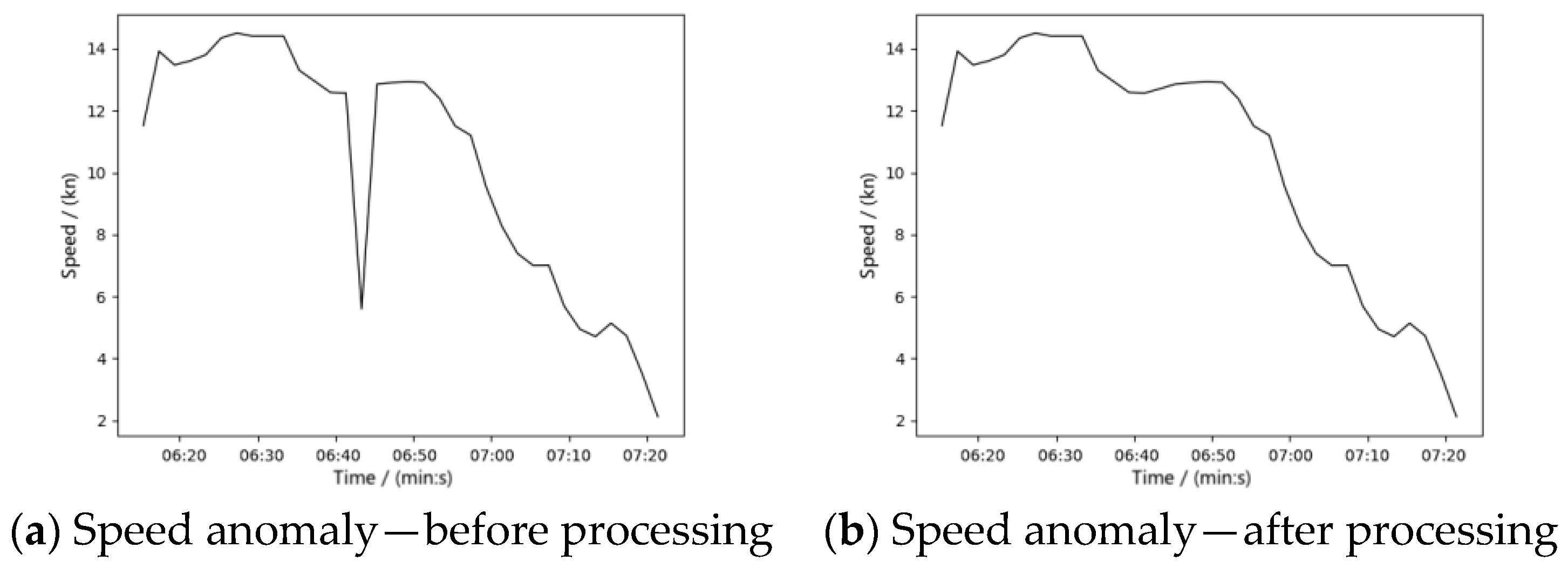
Due to the transmission failure between the AIS and the shore-based system or the improper maintenance of human beings, etc., motion logic errors such as abnormal ship position and speed often appear in the AIS data. As shown in Figure 2a, the speed change can be detected by calculating the average speed between track points by Equation (2).
v ¯ i = ( y i y i + 1 ) 2 + ( x i x i + 1 ) 2 t i + 1 t i
At this time, the ship’s speed should meet the condition given by
v i a ( t i + 1 t i ) v ¯ i v i + a ( t i + 1 t i ) ,
where a and a are the forward and reverse acceleration when the ship is moving forward. Otherwise, the track point is detected as an abnormal speed point, and the average speed between the two points is used to replace the wrong speed data at this point as Equation (4). The repair effect is shown in Figure 2b.
v i = { v i ,   n o r m a l   s p e e d   v ¯ i ,   a b n o r m a l   s p e e d  
For ship position data maintenance, when judging the sudden change of ship position as shown in Figure 3, we use Equations (5) and (6) to detect and repair.
{ x ^ t i + 1 = x i + v i ( t i + 1 t i ) y ^ t i + 1 = y i + v i ( t i + 1 t i )
( x i x i + 1 ) 2 + ( y i y i + 1 ) 2     0 . 5 a ( t i + 1   t i ) 2 ,
where x ^ t i + 1 and y ^ t i + 1 are the estimated position at time t i + 1 , If the ship’s position does not satisfy Equation (6), we use the estimated position to update it.
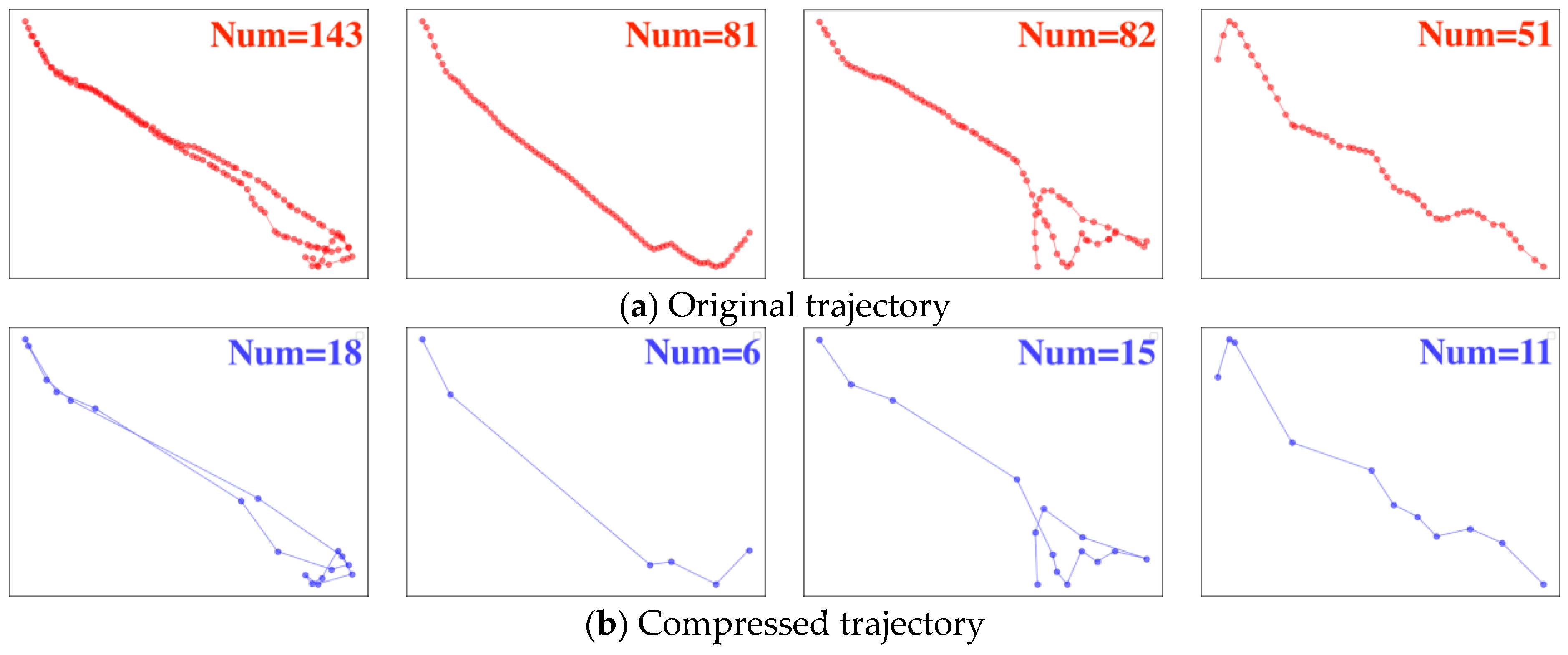
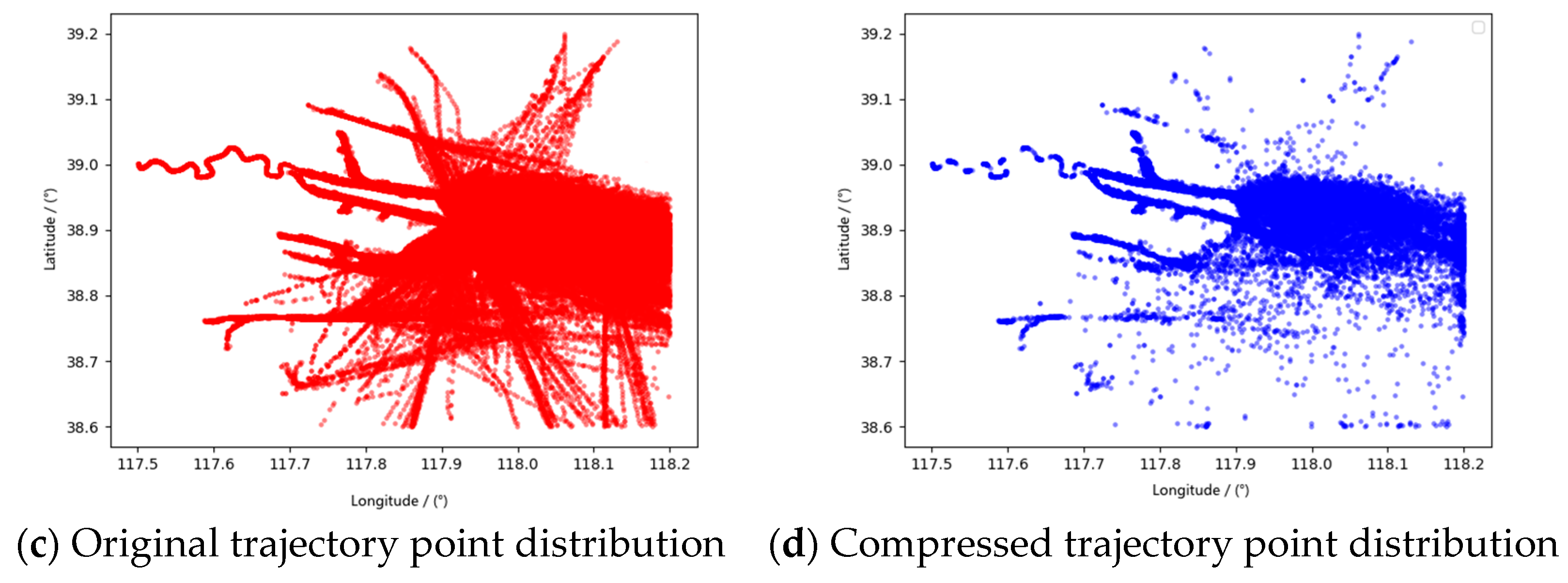
The average daily ship traffic in the port area can reach thousands, and the frequency of broadcasting AIS information is generally 2–30 s, depending on the speed and type of ship. The number of track points in the original data set often reaches millions, and the shipping speed in the port area is generally slow, which is the reason for too much redundant data. Compression of trajectory points is useful for saving data storage and computation costs. The Douglas–Poker (DP) algorithm [26] is commonly used for the compression of trajectory points with the advantages of translation and rotation without distortion. We use the DP algorithm to extract the location feature points and course feature points of a ship’s trajectory [27]. Meanwhile, we introduce the speed change rate as Equation (7) and keep the points whose speed change rate exceeds 0.1 kn/s as the speed feature points. Figure 4 shows the comparison before and after the compression of some sample trajectories.
  C R S = | v i   v i 1 | t i   t i 1

2.2. Trajectory Clustering Method

This section introduces the trajectory clustering model based on the preprocessed AIS data, which divides the ship traffic flow in the sea area into different regular ship movement patterns.
DBSCAN [28,29] is a simple and effective density-based spatial clustering algorithm with noise. It can identify clusters of any shape in noisy spatial data without setting the number of clusters in advance and can solve the problem that similar trajectories are spatially disjoint, which is very suitable for clustering of unlabeled data such as ship trajectories.
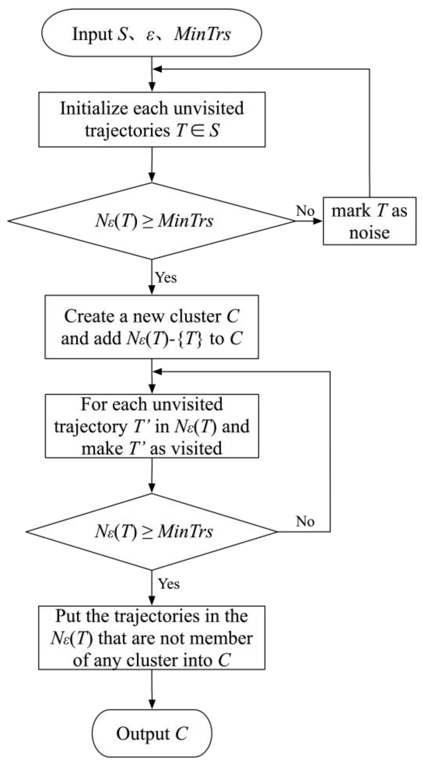
The DBSCAN algorithm uses two parameters:   MinTrs and eps   ( ε ) . MinTrs indicates the minimum number of data (a threshold) clustered together for a region to be considered dense. eps   ( ε ) is a distance measure that will be used to locate objects in the neighborhood of every data. The algorithm proceeds by arbitrarily picking up an object in the dataset S (until all objects have been visited). If there are at least MinTrs objects within a radius of ε to the object then we consider all these objects to be part of the same cluster. The clusters are then expanded by recursively repeating the neighborhood calculation for each neighboring object. The steps of the DBSCAN-based ship trajectory clustering algorithm are shown in Figure 5.
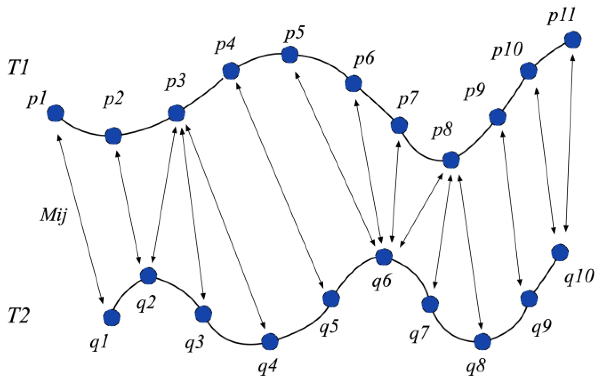
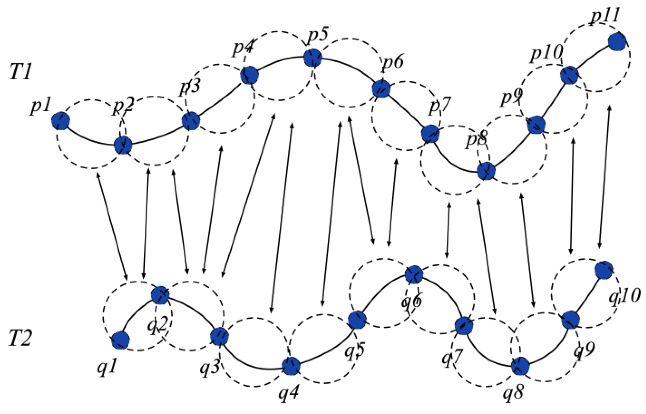
The traditional DBSCAN algorithm performs density clustering in terms of data points. When applying it to ship trajectory clustering, how to calculate the degree of similarity between trajectories is an issue of concern. The broadcasting principle of ship AIS trajectory data leads to different sampling time stamps and sampling quantities, which is a typical kind of unaligned discrete time series data. In this study, we adopted the DTW algorithm to measure the distance between ship tracks. As shown in Figure 6, the principle of DTW is to make the shape between the two sequences as consistent as possible by locally extending or zooming the time series on the time axis and calculating the minimum distance between points on the trajectory sequence to determine the matching combination of track points. In this process, some trajectory points are reused such as q 2 and p 3 . Figure 7 shows all matching trajectory points expressed as a matrix, calculating the shortest Euclidean distance matrix between each point of two trajectory sequences, finding the shortest matching path from the upper left corner to the lower right corner of the matrix, and the sum of all weight values on the twisted path is the DTW distance.
In addition, we summarized the three shortcomings of the DTW algorithm in the ship trajectory similarity metric, namely, the inability to distinguish the local characteristics of the trajectory, the poor ability to distinguish the direction of the trajectory, and the lack of consideration of the starting and ending positions of the trajectory. In this regard, we propose a segmented improved DTW algorithm to solve the above problem. As shown in Figure 8, we improved the point-point matching between two trajectories in the traditional DTW distance to a trajectory sub-segment matching, to improve the ability to distinguish the local features of the ship’s trajectory and the direction of its trajectory. In addition, we adjusted the matching distance weight value of the first and last trajectory sub-segments to improve the sensitivity of the DTW to the position of the ship’s starting and ending trajectory. The steps of the improved algorithm are as follows:
Step 1: Input two trajectory sequences: query trajectory T 1 and compared trajectory T 2 . Define the two trajectory sequences as T 1 = ( p 0 ,   p 1 ,   ,   p m ) and T 2 = ( q 0 ,   q 1 ,   ,   q n ) . p i ( x i ,   y i ) and q j ( x j ,   y j ) to represent the trajectory points in the T 1 and T 2 , and use | T | to represent the length of the trajectory sequence.
Step 2: Connect each two adjacent discrete trajectory points in T 1 and T 2 respectively as trajectory sub-segments, and the sub-segments on T 1 and T 2 are respectively represented as
S i ( p i ,   p i + 1 )   ( 1     i     m 1 )
Step 3: Calculate the point–segment distance, If p i is a trajectory point on the trajectory T 1 , the two ends of the sub-segment S j on T 2 are q j ( x j ,   y j ) and q j + 1 ( x j + 1 ,   y j + 1 ) . Then, the point–segment distance from p i to S j is calculated by
d ps ( p i ,   S j ) = min q S j   d ps ( p i ,   q ) ,
where d ps ( p i ,   q ) represents the Euclidean distance between the two points p i and q .
Step 4: The unidirectional segment–segment distance from S i to S j is defined as the sum of the point–segment distances from the two endpoints of S i to S j divided by the length of S i .
  d ( S i , S j ) = 1 | S i | ( p S i d ps ( p ,   S j ) )
The segment–segment linear distance between S i and S j is equal to the average of the two unidirectional distances:
d ss ( S i ,   S j ) = 1 2 ( d ( S i ,   S j ) + d ( S j ,   S s ) )
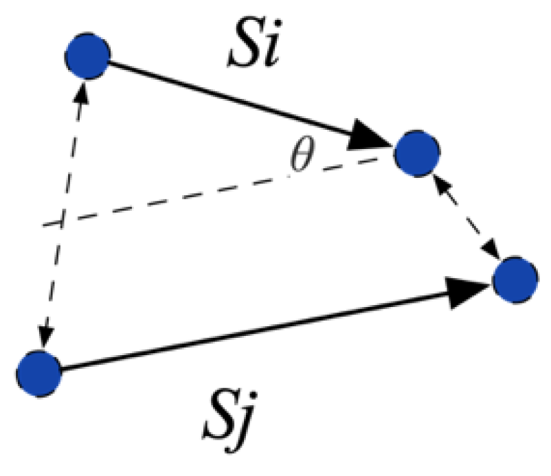
Step 5: The angle θ ( 0   θ   180 ) between S i and S j is shown in Figure 9; it can be calculated by
  θ = | arctan 2 ( y i + 1   y i   ,   x i + 1 x i ) arctan 2 ( y j + 1 y j   ,   x j + 1 x j ) | ,
where the value domain of arctan 2 is [ π , π ] , and its input is not just the tangent, but two values, for example x 1 and x 2 ; the tangent is their ratio x 1 x 2 .
The angular distance between S i and S j is defined as:
d θ ( s i ,   s j ) = { | s i | × sin θ ,   if   0     θ     90 | s i | ,   if   90     θ     180
The segment–segment comprehensive distance can be calculated by
  dist ( s i ,   s j ) = w 1   d ss ( S i ,   S j ) + w 2   d θ ( S i ,   S j )
where w 1 , w 2 respectively represent the weight values of linear and angular distance, which are both set to 0.5 in this study.
Step 6: The dist ( s i ,   s j ) is brought into the DTW algorithm instead of the traditional point matching method to obtain the dynamic time warping distance, which is the similarity degree between T 1 and T 2 .
  DTW ( T 1 ,   T 2 ) = { ,   if   m = 0   or   n = 0 dist ( Head ( T 1 ) ,   Head ( T 2 ) ) + minDTW { ( Rest ( T 1 ) ,   Rest ( T 2 ) ) ,   ( Rest ( T 1 ) ,   T 2 ) ,   ( T 1 ,   Rest ( T 2 ) ) } ,   otherwise    
where m , n respectively represent the number of sub-segments on T 1 and T 2 . Similar to the traditional DTW algorithm,   Head ( T 1 ) represents the first sub-segment on T 1 ; Rest ( T 1 ) represents the remaining sub-segments after removing Head ( T 1 ) from T 1 ; dist ( Head ( T 1 ) ,   Head ( T 2 ) ) represents the segment–to–segment comprehensive distance between Head ( T 1 ) and Head ( T 2 ) .
Step 7: Adjust the weights of the first and last sub-segments of the trajectory. Based on experience, these weight values are set to 2 in this study.
  Distance   weight   = DTW   pair   ×   Weight   T = [ D 1   D 2     D n ] × [ 2 1 1 2 ]
where Weight   T is the influence weight matrix of the track point combination.   Distance   weight   is the combined distance matrix of the trajectory segment after the weight adjustment.

3. Anomalous Ship Behavior Detection Using Recurrent Neural Network

3.1. Bidirectional Gated Recurrent Unit Model

Deep neural networks have powerful extraction and abstraction capabilities that can use a large amount of data for training and learning, and perform deep mapping between input and output data. RNN is a deep learning algorithm specifically designed for spatiotemporal sequential data, but it has the shortcoming of rapid deterioration of neuron node memory. The LSTM model effectively improves this deficiency of RNN. Its memory module contains one or more autocorrelated core cells and three new cell gates for controlling the flow of information into the storage unit and from the unit to the network input gate, output gate and forget gate, which determine which information should be removed from the processor state, precisely through the concept of “gates”.
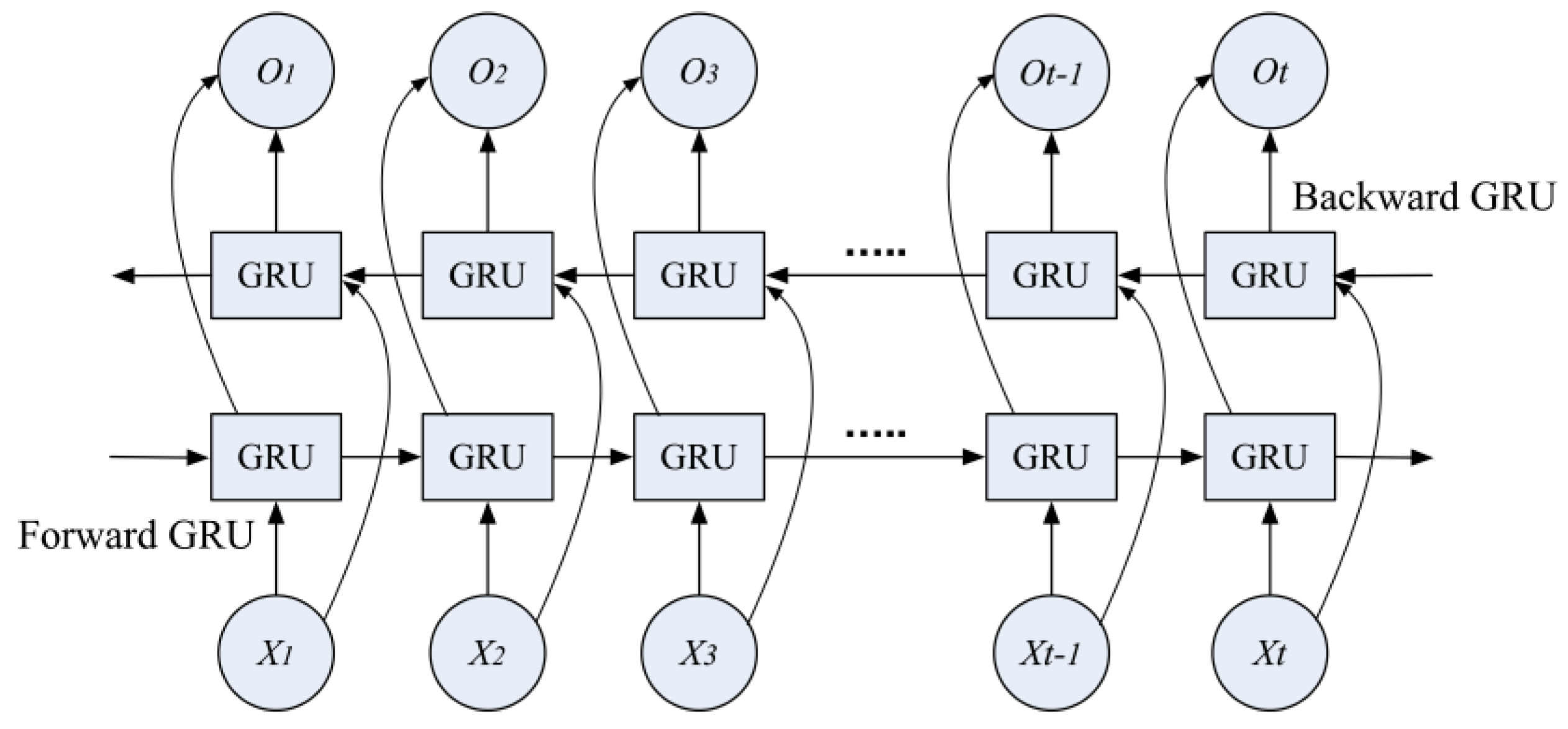
The Gated Recurrent Unit (GRU) is a variant of LSTM developed in recent years, which in essence replaces the hidden units of the RNN with GRU module units as shown in Figure 10, effectively solving the gradient disappearance problem caused by the short-term memory of the ordinary RNN. GRU combines the forget gate and input gate in LSTM into an update gate. The final model has fewer tensors and fewer parameters than the LSTM model, and it is faster than LSTM in terms of running speed and simpler training process.
The GRU module unit calculates the reset gating state r t and the update gating state z t through the input x t of the current node and the output h t 1 of the previous node.
r t = σ ( W r     [ h t 1 ,   x t ] )
z t = σ ( W z     [ h t 1 ,   x t ] )
After getting the signal, first, get the reset data by multiplying h t 1 and r t , and then splice with the x t , and use the tanh activation function to scale the data to the range of [−1, 1] to get the current hidden state h .
h ˜ t = t a n h ( W h ˜ [ r t h t 1 , x t ] )
“Update memory” is the core calculation step of GRU. Forgetting and memory are carried out at the same time. The previously obtained update gate z is used as the forgetting gate, 1     z is used as the input gate, and the expression is updated as in Equation (20). This is the biggest difference from LSTM because GRU uses the same gate to control z , and accomplishes forgetting and memory at the same time. The gate control signal z [ 0 ,   1 ] , the closer its value is to 0, the more the data is forgotten; conversely, the closer it is to 1, the more data it retains.
h t = z t h ˜ t + ( 1 z t ) h t 1
W z , W r and W h ˜ denote the weight matrices of the GRU neural network training at time t. They consist of the following two weight matrices, respectively.
W z = W z x + W z h ˜
W r = W r x + W r h ˜
W h ˜ = W h ˜ x + W h ˜ h ˜ ,
where W zx , W rx , and W h ˜ x are the weight matrix from the input value to the update gate, the reset gate, and the candidate value, respectively. W z h ˜ , W r h ˜ , and W hh ˜ are the weight matrix from the last candidate value to the update gate z t , the reset gate r t , and the candidate’s value h ˜ respectively.
In the above-mentioned models such as LSTM and GRU, the states are transmitted unidirectionally, and the mapping output of the neural network in this case is only based on the forward information of the temporal data. In this study, we adopt the BiGRU to build a ship trajectory prediction model. The structure of the BiGRU neural network is shown in Figure 11, where each training sequence in the BiGRU layer passes through two networks, forward and backwards respectively, and both networks are connected to the same output. This structure not only relies on the above information to adjust the neural network, but also can use the following information to adjust the network with feedback to improve the efficiency of weight update, and thus effectively improve the ship trajectory prediction effect.

3.2. Method for Detecting Abnormal Ship Behavior

The basic principle of the method in this study is to train the RNN using the results from the DBSCAN algorithm. Based on the previous trajectory points and historical traffic patterns, the RNN can be used as a real-time predictor of the ship’s normal trajectory. By judging the deviation of the actual trajectory from the predicted normal trajectory, it can detect whether the ship is sailing abnormally. The advantage of this method is that it does not realize abnormality detection by comparing with the normal trajectory model but carries out autonomous normal trajectory state recognition based on the learning characteristics of the deep neural network itself, and thus achieves more accurate trajectory anomaly detection. At the same time, it becomes very sensitive to the inefficiency of its prediction for trajectories that do not fit the historical regular movement patterns in the sea area. This is the reason why the neural network is chosen as a predictor in this study, and it will also predict differently for different degrees of anomalous behavior.
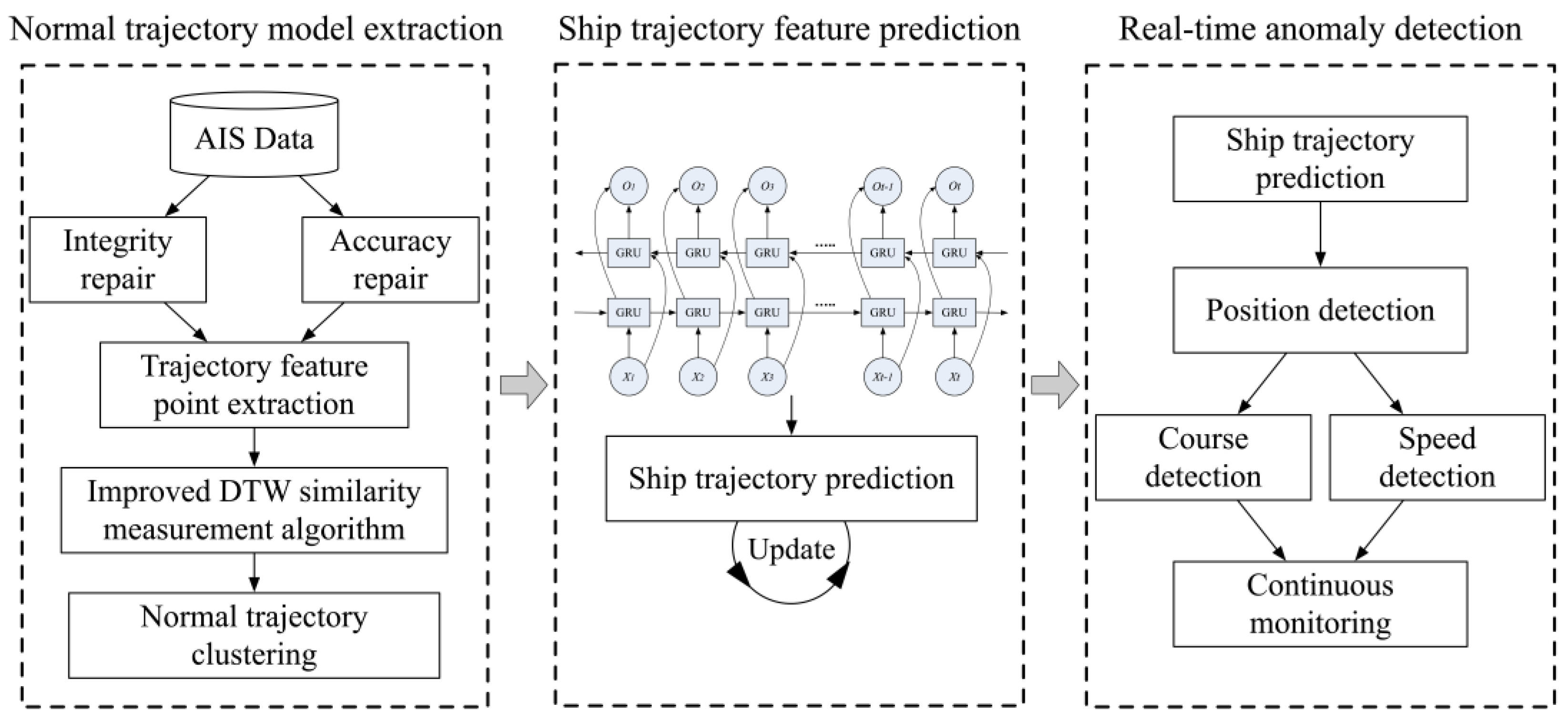
The framework of a ship’s abnormal behavior detection model established in this study is shown in Figure 12. The realization of the trajectory state real-time detection method mainly includes the following steps:
Step 1: Collect the AIS historical trajectory data in the monitored sea area; use the method in Section 3.2 to preprocess the AIS data, and then use the DBSCAN to extract the ship trajectory normal model.
Step 2: The normal trajectory clusters obtained by DBSCAN are used as the training objects of RNN to realize the prediction of the normal state of the ship at the next moment. The trajectory data set includes longitude ( lon ), latitude ( lat ), speed ( sog ), heading ( cog ). For a single trajectory, its trajectory feature at t moment is expressed as:
  Y ( t ) = {   lon ,   lat ,   sog ,   cog   }
In the process of the RNN training and prediction result output, we use a sliding window method to generate the input and output set. The ship’s normal trajectory prediction model can be defined as
Y ( t + 1 ) ,   ,   Y ( t + m ) = f 2 ( { Y ( t n + 1 ) ,   ,   Y ( t 2 ) ,   Y ( t 1 ) ,   Y ( t ) } )
where n is the time step length of the input layer, and m is the step length of the predicted output.
Step 3: Through the ship’s previous navigation status and historical data in the water area, the next stage of the ship’s normal navigation status is predicted. In the actual navigation situation, most of the abnormal behaviors of ships are manifested in the three aspects of the ship’s position, speed, and course. Therefore, this study sets the standard of anomaly detection as the deviation value of a ship’s position, course, and speed, which is defined as:
  deviation _ value = {   GeoDistance   ( pos pre ,   pos act ) | v pre   v act   | | c pre   c act   |
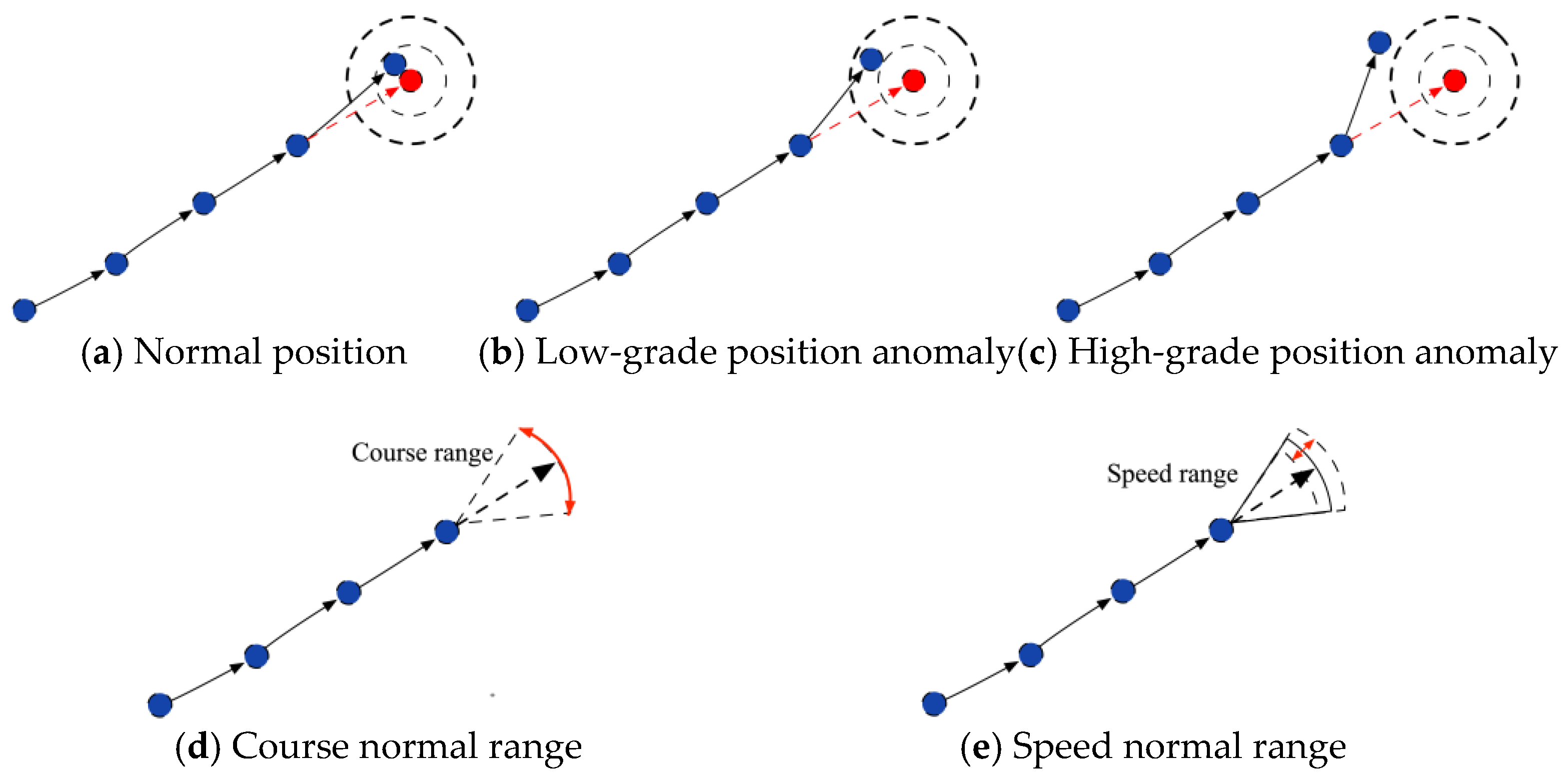
As shown in Figure 13, for the abnormal detection alarm, users can determine the alarm threshold of the deviation values of the ship position, speed, and course according to the actual demand and the performance of the network training. In particular, we set high and low thresholds for position detection, because ship position is the most intuitive representation of a ship’s navigation status. Our model warns the maritime traffic supervisors when the real-time ship data deviates from the high level or continuously exceeds the low-level thresholds. On the contrary, if the prediction results of the ship’s trajectory are accurate, it is considered to be in normal sailing condition.

4. Experiment and Analysis

4.1. Experimental Data and Preprocessing

The data used in this study are the AIS data of China’s Tianjin Port area for two months in 2019. All of the AIS data from cargo ships and tankers were selected as experimental data. The original data content is shown in Table 2. After preprocessing, 11,357 trajectories from 2608 different ships were retained out of the original dataset of 712,214 track points. In the original data, 30.3% of the data has insufficient integrity. In the process of trajectory accuracy repair, 1.76% of the trajectory points had character errors, and it was detected that 0.67% of the trajectory points had motion logic errors; The trajectory compression ratio is 62.46%, and the final output is 267,365 key feature points of the AIS trajectory. The detailed processing information is shown in Table 3, Table 4 and Table 5.
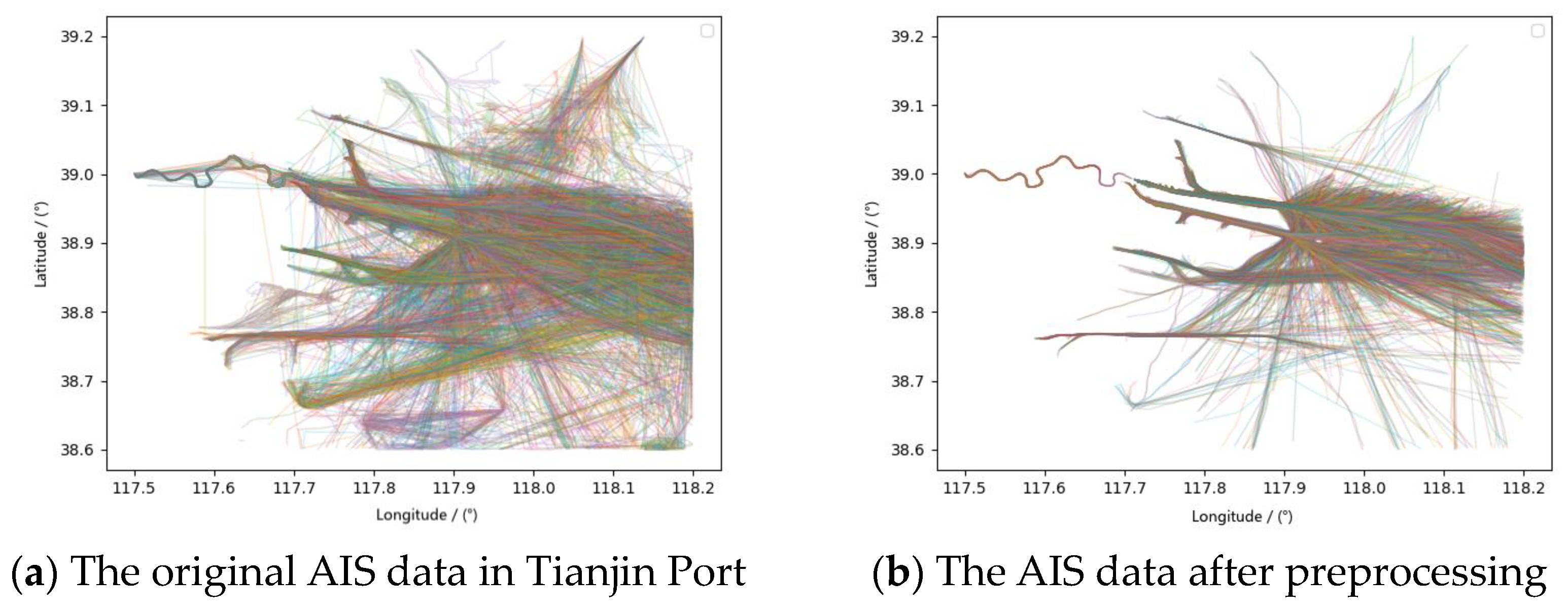
The preprocessing effect is shown in Figure 14. It can be seen that the messy trajectory and trajectory drift in the original data have been eliminated, and some phenomena that obviously did not conform to the logic of kinematics and navigational practices (crossing the land, trajectory mutations, etc.) have been resolved. While effectively compressing the number of ship trajectory points, the original ship trajectory features are retained.

4.2. Clustering Analysis

In order to verify the accuracy and clustering effect of the segmented improved DTW algorithm, we conducted a clustering comparison experiment of the improved DTW, DTW and Hausdorff. The experimental data set contains 334 ship trajectories, as shown in Figure 15. These trajectories have obvious differences in shape, direction, and ship starting and ending points. They are pre-marked as 8 trajectory clusters.
The DBSCAN algorithm is very sensitive to the selection of the neighborhood and the density threshold. The choice of parameters will directly affect the accuracy of clustering results. Through the parameter combination adaptive method [30], ε = 0.3   nm , MinTrs = 3 are determined, in which the clustering effect of the density clustering algorithm reaches a more desirable state.
Figure 16 shows the DBSCAN clustering effect based on three different distance measurement methods. The trajectory sets of different colors represent different clusters, and the noise trajectory is not shown.
We use the clustering error rate (ER) to evaluate the clustering results. The error rate is defined as
  ER = 1 1 N c = 1   k p c  
where N is the total number of all trajectories, K is the number of correct trajectory clusters, and p c is the number of correct trajectories in cluster c . The lower the ER , the higher the accuracy of the clustering algorithm. The evaluation of trajectory clustering results is shown in Table 6.
The experimental results show that the trajectory clustering result of the improved DTW is eight types of clusters, which is basically consistent with the pre-labeled trajectory clusters. The clusters with local shape feature differences (cluster 1 and cluster 2 and cluster 4) and the trajectory sets with different start and end positions (cluster 2 and cluster 3 and cluster 6, cluster 7 and cluster 8) are more accurately identified. The trajectory clustering result of DTW is six types of cluster, and the clustering error rate is 8.7%. Some local shape features and starting and ending location features are ignored, and cluster 1 and cluster 2 cluster 7 and cluster 8, are identified as the same cluster. The clustering effect based on Hausdorff is the worst. The clustering result is four clusters, and the clustering error rate reaches 17.9%. Some trajectories in the opposite direction and large local shape differences are not recognized.

4.3. Ship Abnormal Behavior Detection Experiment

4.3.1. Ship Navigation State Prediction

As described in Section 3.2, we divide the trajectory clusters obtained by the DBSCAN clustering algorithm at a ratio of 75% and 25% and use them as the training set and test set to train BiGRU. And the time interval of the trajectory points in the data set is regularized to 2 min. To reduce the prediction error caused by the difference in magnitude, all data values are normalized before training.
Table 7 shows the experimental environment of this study. After comparative experiments and manual adjustments, the optimal parameter combination of the BiGRU was finally determined. The time step of the input data obtained by the sliding window method is 5, and the time step of the output is 1. This means that in our method, the state of the ship at the next moment is also measured based on the five previous trajectory points. In order to judge the prediction effect more intuitively, we use the deviation between the predicted ship’s position, speed, course and the actual value to evaluate the prediction model.
Figure 17 shows the detailed results of ship position predictions of two real historical trajectories selected from the test set. The black arrow represents the direction of the ship’s trajectory. It can be seen that the predicted trajectory is highly coincident with the actual situation, and the non-linear behavior of the ship such as steering and speed change can be accurately predicted. Table 8 and Table 9 show the prediction error results of these two test trajectories based on BiGRU, GRU and LSTM respectively, and it can be seen that BiGRU performs better than GRU and LSTM in terms of the average and maximum error in predicting the trajectory position, course and speed characteristics.
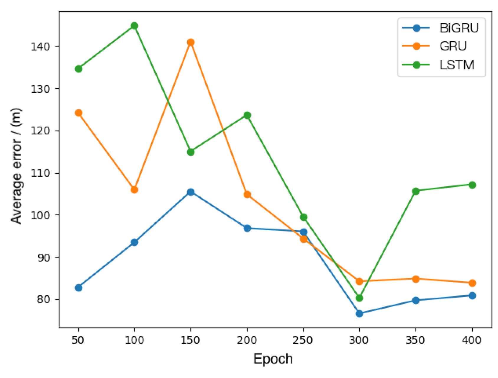
Figure 18 compares the average prediction error of BiGRU, GRU and LSTM neural network models with a different number of iterations based on the test set data, and the prediction errors of LSTM and GRU fluctuate widely with the number of iterations, while the prediction error of BiGRU is relatively stable, and the average error of ship position is basically controlled under 90 m. The prediction accuracy of the three methods showed an overall trend of BiGRU > GRU > LSTM, and BiGRU reduced the average prediction error by 13.1% compared with GRU and 21.3% compared with LSTM.

4.3.2. Ship Abnormal Behavior Detection

In this study, we consider vessel trajectory states that do not comply with the traffic patterns in the water as vessel anomalous behaviour, and three aspects are monitored: position, speed and course. Following the method in Section 3.2, we set the low threshold for ship position detection to 100 m and the high threshold to 250 m, and the anomaly thresholds for both heading and speed to ±3% of the predicted normative values.
As shown in Figure 19, in this experiment four real trajectories were chosen to verify the anomaly detection capability of the proposed method, and the detailed descriptions of the four tracks are shown in Table 10.
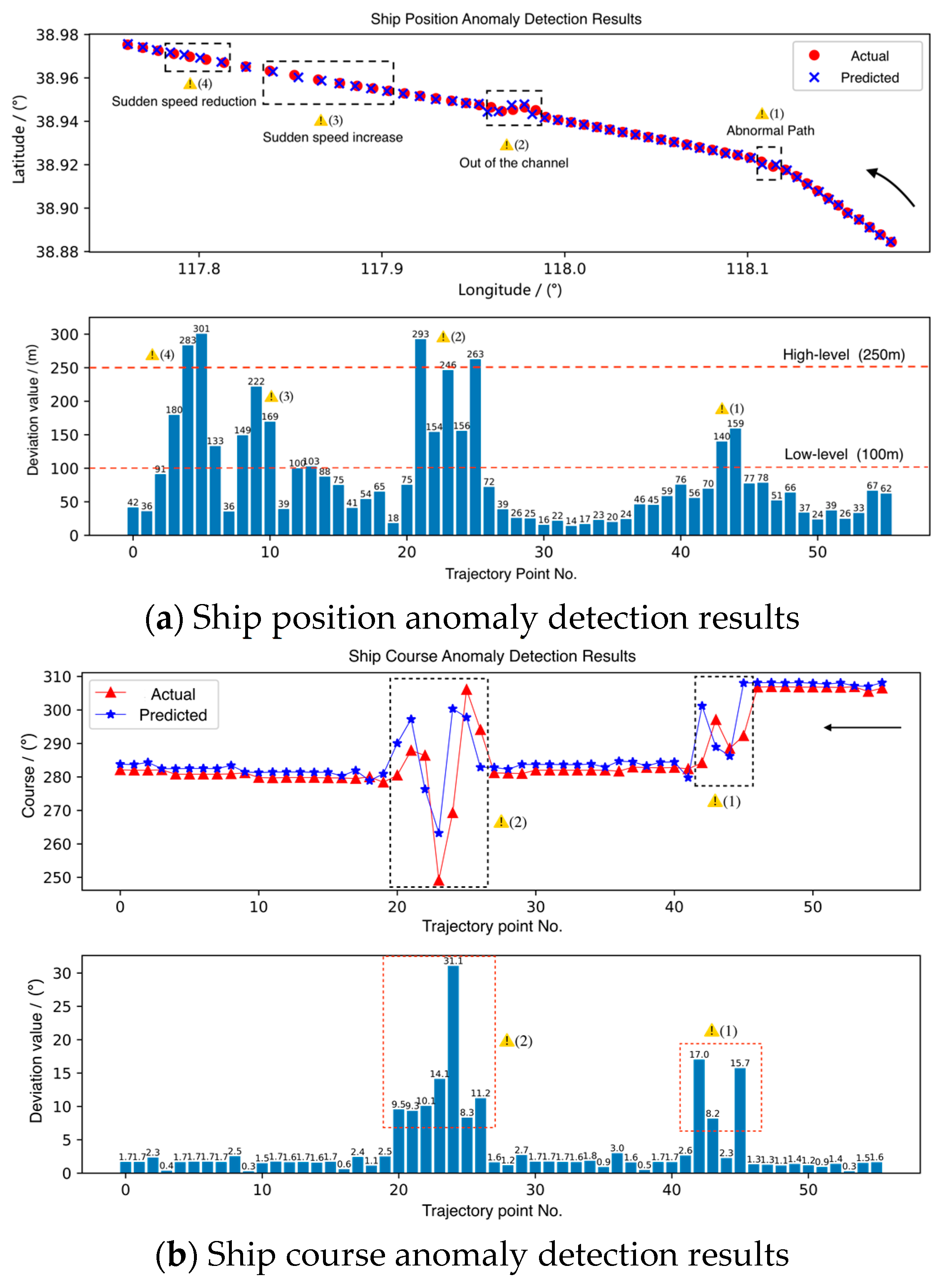
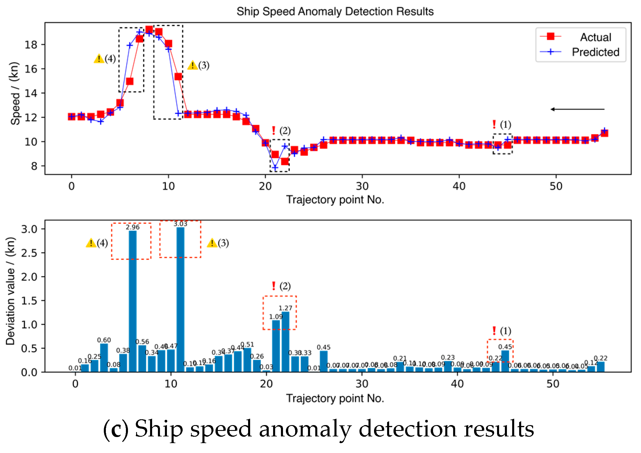
Figure 20 shows the abnormal detection detailed results for “Trajectory No.1”. The black arrow represents the direction of the ship’s trajectory. The real-time details of the anomaly warnings during the ship navigation are shown in Table 11. It can be seen that the trajectory does not follow the prescribed route at the channel turning point, but sails into a reverse route, and the change of the trajectory point heading is 292.3 at 12:32, which is beyond the predicted normal course range and triggers the trajectory heading anomaly warning, and then (12:34–12:36) the change of its course continues to cause a large deviation of the ship position from the real-time predicted normal trajectory. The low-grade trajectory position anomaly warning is triggered until 12:40 when the ship resumed normal sailing status and the anomaly Alert (1) ended.
During the navigation in the main channel, at 13:10, the ship turned to the right sharply, and then (13:12) the predicted normal position of the trajectory was still in the channel, while its real position had already sailed out of the channel, which triggered the high-grade trajectory position anomaly warning, and then, (13:12–13:20) the ship’s course was still in an unstable abnormal state, and the position anomaly warning was continuously triggered until 13:22 when the ship returned to the normal the abnormal Alert (2) ends. In addition, the abnormal fluctuation of ship speed caused by abnormal ship steering is also successfully detected and recognized in the abnormal Alert (1) and abnormal, Alert (2).
At 13:40, although the ship was traveling along a normal course in the channel, the normal trajectory speed predicted by the model was 12 kn at this time, its real speed increased abruptly by 3.2 kn in 2 min, triggering the abnormal speed warning. This abnormal variable speed behavior is against good seamanship and may affect the traffic flow across the channel, causing the potential danger of marine traffic accidents. Then, its speed continued to increase abruptly causing its trajectory to continuously deviate from the predicted normal position, triggering an abnormal trajectory position, Alert (3). Subsequently, at 13:50, the ship’s speed plummeted by 3.6 kn, triggering the abnormal Alert (4).
The results of the abnormal ship trajectory of “Trajectory No.1” above show that the proposed method can detect the abnormal navigation behavior of the ship in time and accurately from the three aspects of ship trajectory point position, speed and course.
We believe that the core goal of ship abnormal behavior detection is to accurately issue an alarm within the shortest time at the moment of abnormal occurrence, so as to prevent the dangerous situation from deteriorating as much as possible in a timely and effective manner. Therefore, we introduce three indicators to evaluate the experimental results: trajectory detection accuracy rate, trajectory detection false rate and alarm timeliness.
The detection accuracy rate (AR) refers to the ratio of the abnormal trajectory points detected by the algorithm to the actual abnormal trajectory points in the process of ship trajectory abnormality detection, which is calculated as Equation (28).
AR = 1 N M   ×   100 %
where M is the actual number of abnormal trajectory points in the ship navigation and N is the number of undetected abnormal trajectory points.
The detection false rate (FR) alarm rate refers to the ratio of normal track points that are incorrectly identified as abnormal track points. It is calculated as Equation (29). M t indicates the number of normal trajectory points of the trajectory, and N f indicates the number of misidentified abnormal trajectory points.
FR = N f M t   ×   100 %
Detection timeliness refers to whether the ship trajectory anomaly detection algorithm can recognize the occurrence of trajectory anomaly in time and the computing time consuming of the algorithm, which can measure the real-time anomaly detection ability of the algorithm.
Table 12, Table 13 and Table 14 show the evaluation of the experimental results for the three models, respectively. It can be seen that in the detection process of four experimental trajectories, the average detection accuracy of BiGRU-based and GRU-based trajectory anomaly detection is higher at 96.35% and 93.23%, respectively. In addition, the LSTM-based fails to effectively identify some of the abnormal trajectory points, with an average detection accuracy of 88.15%.
In terms of detection false alarm rate, the BiGRU model only misidentified three trajectory points in “Track No.1”, while the average false alarm rates for GRU and LSTM were relatively high at 6.46% and 9.79%, respectively.
In terms of detection timeliness, a total of nine anomalous behaviors occurred in the four simulated voyages, and the number of timely recognitions was nine for the BiGRU trajectory anomaly detection model and eight for both GRU and LSTM. Moreover, as the number of experimental trajectory points increases, the Time Consuming of the BiGRU model increases less, and the real-time performance of trajectory anomaly detection is better.
The experiments show that the proposed method can detect the abnormal behavior of the ship in three aspects: position, speed and heading in a timely and effective manner.

5. Conclusions

Maritime traffic monitoring based on maritime data and computer technology can overcome the limitations of traditional methods in terms of the inexperience and physical fatigue of supervisors. It can also improve the level of intelligence of maritime supervision, provide valuable information about the maritime traffic situation, assist in dangerous supervision, reduce the occurrence of maritime accidents and illegal acts, and optimize the efficiency of traffic flow. In this paper, we take the ship trajectory data broadcasted by the AIS as the research object and propose a ship trajectory anomaly detection method with AIS trajectory data as the driver, ship trajectory clusters as the normal model, and deep neural network as the anomaly detection tool.
The contribution of this study is threefold. Firstly, the data quality issues in real AIS data are analyzed, and three aspects of AIS data quality are summarized, including spatial and temporal integrity, physical accuracy, and data conciseness. To overcome these problems, a complete set of general trajectory pre-processing methods is proposed, mainly including ship trajectory segmentation expression, base abnormality repair, position abnormality repair, and speed abnormality repair. The spatio-temporal feature points in the ship trajectory are extracted to ensure the compression rate, while the features of the original trajectory are highly restored, which effectively saves the computational cost of data mining.
Secondly, it uses the advanced unsupervised machine learning model DBSCAN algorithm for extracting higher quality maritime normative traffic models. In particular, in order to measure the similarity between trajectories more accurately, this study improves the traditional DTW algorithm to be able to identify the direction, local shape features and start and stop location of trajectories. In the comparison experiments, the accuracy of the improved DTW algorithm reached 99.42%, which is much higher than that of the ordinary DTW and Hausdorff, verifying the performance of the proposed method.
Thirdly, we build a ship trajectory prediction model based on BiGRU to solve the problem of gradient disappearance and gradient explosion of RNN and make the prediction model consider the contextual information of trajectory information to effectively improve the accuracy of prediction. Moreover, it is used as a detector to comprehensively judge the position, heading and course of the ship during navigation, and realize the real-time abnormal detection of a ship heading in the water. We also compared BiGRU with two other deep learning algorithms, LSTM and GRU, both of which showed some missed and false alarms and untimely alarms, while BiGRU achieved 96.35% accuracy in anomaly detection and only 1.67% false alarm rate, and timely warning of anomalous ship behavior. This verifies the superior performance of our proposed method in detecting abnormal ship behavior.
However, this method requires a high-quality sample trajectory model, such as data pre-processing, normal trajectory clustering and neural network training to have an impact on the detection effect. In the data pre-processing, some data that cannot match dynamic and static information, as well as those with fewer valid trajectory points are eliminated, and the repair of such data can be considered in future research to achieve the optimal utilization of AIS information mining. The normal model in this study only selects cargo ships and tankers, and shorter ships, such as fishing vessels, should be considered in the future, which is more effective for anomaly detection in specific waters. To meet the practical application requirements, the adaptive capability of updating the normal model to integrate new data should also be strengthened. In addition, in practice, ship behavior is related to the spatial and temporal context in which the ship is located at the moment, including the interaction of other ships around, weather conditions, sea state and other factors. Correlating spatio-temporal semantic analysis of ship navigation environment with ship behavior anomaly detection is also one of the future research priorities.

Author Contributions

Conceptualization, B.Z., K.H., H.R., D.W.; methodology, B.Z., H.R.; data curation, B.Z., D.W.; software, B.Z., H.L.; writing—original draft preparation, B.Z.; writing—review and editing, B.Z., K.H.; supervision, K.H. All authors have read and agreed to the published version of the manuscript.

Funding

This research was funded by China Scholarship Council, grant Number 202106570007.

Institutional Review Board Statement

Not applicable.

Informed Consent Statement

Not applicable.

Data Availability Statement

Not applicable.

Conflicts of Interest

The authors declare no conflict of interest.

References

  1. International Maritime Organization (IMO). Resolution MSC. 74 (69): Adoption of New and Amended Performance Standards; International Maritime Organization (IMO): London: UK, 1998. [Google Scholar]
  2. Sidibé, A.; Shu, G. Study of automatic anomalous behavior detection techniques for maritime vessels. J. Navig. 2017, 70, 847–858. [Google Scholar] [CrossRef]
  3. Laxhammar, R. Anomaly detection for sea surveillance. Information Fusion. In Proceedings of the 11th International Conference on Information Fusion, Cologne, Germany, 30 June–3 July 2008; pp. 1–8. [Google Scholar]
  4. Iphar, C.; Ray, C.; Napoli, A. Data integrity assessment for maritime anomaly detection. Expert Syst. Appl. 2020, 147, 113219. [Google Scholar] [CrossRef]
  5. Martineau, E.; Roy, J. Maritime Anomaly detection: Domain Introduction and Review of Selected Literature; Technical Report; Defense Research and Development Canada—Valcartier, Technical Memorandum TM2010-460; Defence Research and Development Canada: Ottawa, ON, Canada, 2011. [Google Scholar]
  6. Riveiro, M.; Pallotta, G.; Vespe, M. Maritime anomaly detection: A review. Data Min. Knowl. Discov. 2018, 8, e1266. [Google Scholar] [CrossRef] [Green Version]
  7. Wolsing, K.; Roepert, L.; Bauer, J.; Wehrle, K. Anomaly Detection in Maritime AIS Tracks: A Review of Recent Approaches. J. Mar. Sci. Eng. 2022, 10, 112. [Google Scholar] [CrossRef]
  8. Chandola, V.; Banerjee, A.; Kumar, V. Anomaly detection: A survey. ACM Comput. Surv. 2009, 41, 75–79. [Google Scholar] [CrossRef]
  9. Wang, Y.; Liu, J.; Liu, R.W.; Liu, Y.; Yuan, Z. Data-driven methods for detection of abnormal ship behavior: Progress and trends. Ocean. Eng. 2023, 271, 113673. [Google Scholar] [CrossRef]
  10. Holst, A.; Ekman, J. Anomaly Detection in Vessel Motion; International Report Saab Systems: Järfälla, Sweden, 2003. [Google Scholar]
  11. Ristic, B.; Scala, B. Statistical analysis of motion patterns in AIS data: Anomaly detection and motion prediction. In Proceedings of the 11th International Conference on Information Fusion, Cologne, Germany, 30 June–3 July 2008; pp. 109–122. [Google Scholar]
  12. Xiao, F.; Ligteringen, H.; Van Gulijk, C.; Ale, B. Comparison study on AIS data of ship traffic behavior. Ocean. Eng. 2015, 95, 84–93. [Google Scholar] [CrossRef] [Green Version]
  13. Rong, H.; Teixeira, A.P.; Guedes, S. Ship trajectory uncertainty prediction based on a Gaussian Process model. Ocean. Eng. 2019, 182, 499–511. [Google Scholar] [CrossRef]
  14. Vespe, M.; Visentini, I.; Bryan, K.; Braca, P. Unsupervised learning of maritime traffic patterns for anomaly detection. In Proceedings of the 9th IET Data Fusion & Target Tracking Conference: Algorithms & Applications, London, UK, 16–17 May 2012; pp. 1–5. [Google Scholar]
  15. Mascaro, S.; Nicholso, A.E.; Korb, K.B. Anomaly detection in vessel tracks using Bayesian networks. Int. J. Approx. Reason. 2014, 55, 84–98. [Google Scholar] [CrossRef]
  16. Lei, P.R. A framework for anomaly detection in maritime trajectory behavior. Knowl. Inf. Syst. 2016, 47, 189–214. [Google Scholar] [CrossRef]
  17. de Souza, E.N.; Boerder, K.; Matwin, S.; Worm, B. Improving fishing pattern detection from satellite AIS using data mining and machine learning. PLoS ONE 2016, 11, e0158248. [Google Scholar]
  18. Toloue, K.F.; Jahan, M.V. Anomalous behavior detection of marine vessels based on Hidden Markov Model. In Proceedings of the 6th Iranian Joint Congress on Fuzzy and Intelligent Systems (CFIS), Kerman, Iran, 28 February–2 March 2018; pp. 10–12. [Google Scholar]
  19. Laxhammar, R.; Falkman, G. Online learning and sequential anomaly detection in trajectories. Trans. Pattern Anal. Mach. Intell. 2014, 36, 1158–1173. [Google Scholar] [CrossRef] [PubMed]
  20. Bomberger, N.A.; Rhodes, B.J.; Seibert, M. Associative learning of vessel motion patterns for maritime situation awareness. In Proceedings of the 9th International Conference on Information Fusion, Florence, Italy, 10–13 July 2006; Volume 54, pp. 1–8. [Google Scholar]
  21. Zhao, L.B.; Shi, G.Y. Maritime anomaly detection using density-based clustering and recurrent neural network. J. Navig. 2019, 72, 894–916. [Google Scholar] [CrossRef]
  22. Tang, H.; Yin, Y.; Shen, H.L. A model for vessel trajectory prediction based on long short-term memory neural network. J. Mar. Eng. Technol. 2022, 21, 136–145. [Google Scholar] [CrossRef]
  23. Tang, H.; Wei, L.Q.; Yin, Y.; Shen, H.; Qi, Y. Detection of abnormal vessel behavior sased on probabilistic directed graph model. J. Navig. 2022, 21, 136–145. [Google Scholar]
  24. Zhen, R.; Jin, Y.; Hu, Q.Y. Vessel behavior prediction based on AIS data and BP neural network. Navig. China 2017, 40, 6–10. [Google Scholar]
  25. Zhao, L.B.; Shi, G.Y.; Yang, J.X. Ship trajectories pre-processing based on AIS data. J. Navig. 2018, 71, 1210–1230. [Google Scholar] [CrossRef]
  26. Douglas, D.H.; Peucker, T.K. Algorithms for the reduction of the number of points required to represent a digitized line or its caricature. Int. J. Geogr. Inf. Geovisualization 1973, 10, 112–122. [Google Scholar] [CrossRef] [Green Version]
  27. Fikioris, G.; Patroumpas, K.; Artikis, A.; Pitsikalis, M.; Paliouras, G. Optimizing vessel trajectory compression for maritime situational awareness. GeoInformatica 2022, 27, 1–27. [Google Scholar] [CrossRef]
  28. Ester, M.; Kriegel, H.P.; Sander, J.; Xu, X. A density-based algorithm for discovering clusters in large spatial databases with noise. In Proceedings of the KDD-96 Proceedings, Portland, Oregon, 2–4 August 1996; Volume 96, pp. 226–231. [Google Scholar]
  29. Pallotta, G.; Vespe, M.; Bryan, K. Vessel pattern knowledge discovery from AIS data: A framework for anomaly detection and route prediction. Entropy 2013, 15, 2218–2245. [Google Scholar] [CrossRef] [Green Version]
  30. Zhao, L.B.; Shi, G.Y. A trajectory clustering method based on douglas- peucker compression and density for marine traffic pattern recognition. Ocean. Eng. 2019, 172, 456–467. [Google Scholar] [CrossRef]
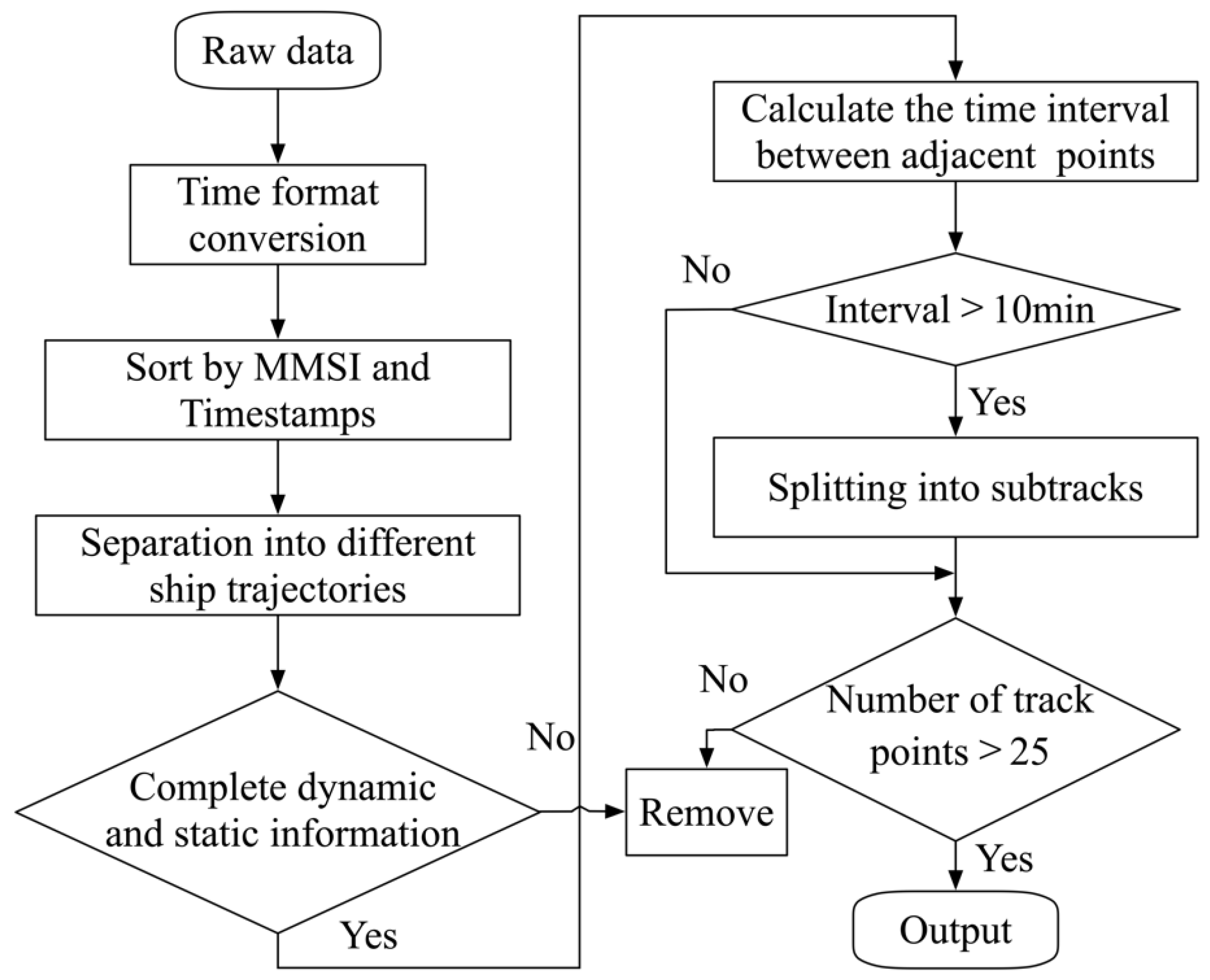
Figure 1. Trajectory integrity processing steps.
Jmse 11 00763 g001
Figure 2. Trajectory point speed anomaly repair effect.
Jmse 11 00763 g002
Figure 3. Trajectory point position anomaly repair effect.
Jmse 11 00763 g003
Figure 4. Trajectory point compression effect.
Jmse 11 00763 g004
Figure 5. DBSCAN-based ship trajectory clustering algorithm.
Jmse 11 00763 g005
Figure 6. Trajectory point matching method in DTW algorithm.
Jmse 11 00763 g006
Figure 7. Schematic diagram of Dynamic Time Warping Distance.
Jmse 11 00763 g007
Figure 8. Schematic diagram of dynamic matching of segmented DTW algorithm.
Jmse 11 00763 g008
Figure 9. Diagram of angular distance between trajectory segments.
Jmse 11 00763 g009
Figure 10. Schematic diagram of trajectory prediction model based on GRU.
Jmse 11 00763 g010
Figure 11. Schematic diagram of BiGRU.
Jmse 11 00763 g011
Figure 12. Process of the proposed ship abnormal behavior detection method.
Jmse 11 00763 g012
Figure 13. Schematic diagram of abnormal detection of ship position, course and speed.
Jmse 11 00763 g013
Figure 14. AIS trajectory pre-processing effect in Tianjin Port.
Jmse 11 00763 g014aJmse 11 00763 g014b
Figure 15. Clustering Experiment data.
Jmse 11 00763 g015
Figure 16. Clustering effect comparison based on three trajectory similarity measurement methods.
Jmse 11 00763 g016
Figure 17. Real AIS trajectory prediction results.
Jmse 11 00763 g017
Figure 18. Comparison of prediction errors between BiGRU, GRU and LSTM.
Jmse 11 00763 g018
Figure 19. Anomaly detection experiment trajectories.
Jmse 11 00763 g019
Figure 20. Detailed prediction and detection results.
Jmse 11 00763 g020aJmse 11 00763 g020b
Table 1. Major features of preceding studies.
MethodPublicationsUse Attributes of Ship Behavior DataDetection Model
Authors
Statistical AnalysisHolst [10]Ship Location, SpeedGaussian Distribution
Laxhammar et al. [3]Ship Location, SpeedGMM
Ristic et al. [11]Ship LocationKDE
Xiao [12]Lateral Position, Speed, Course and Time IntervalStatistical Distribution
Rong et al. [13]Ship Location, Speed and TimestampGaussian Process
Machine LearningVespe [14]Ship Location, Speed and CourseUnsupervised Learning
Mascaro [15]Ship Location, Speed, Course and Spatio-temporal Contextual Information Bayesian Network
Lei [16]Ship LocationMT-MAD
Souza [17]Ship Location, Speed and Operating TimeHidden Markov Model, Data Mining and Multilayer filtering Strategy
Toloue [13]Ship Location, Speed and CourseHidden Markov Model
Prediction BasedLaxhammer [14]Ship Location, Speed and TimestampConformal Prediction
Bomberger [15]Ship MMSI, Location, Speed and CourseAssociative Neural Network
Zhao [16]Ship MMSI, Location, Speed, Course and TimestampLSTM
Tang [17,18]Ship MMSI, Location, Speed, Course and TimestampLSTM
This StudyShip MMSI, Location, Speed, Course and TimestampBiGRU
Table 2. The size of raw data in the research area.
Number of Dynamic InformationNumber of Static and Voyage-Related InformationNumber of ShipsNumber of Ships with Additional Information
1,059,741376,33338842556
Table 3. Trajectory integrity repair results.
Quality IssuesNumber of Points RemovedPercentage
Information mismatch169,87616.00%
Insufficient spatial integrity151,55314.30%
Table 4. Trajectory accuracy repair results.
Quality IssuesNumber of Abnormal Track PointsPercentage
AIS data field error18,9101.76%
Location error54520.51%
Speed error17360.16%
Table 5. Trajectory simplicity improvement results.
Processing MethodNumber of Track Points after CompressionCompression Rate
Feature point extraction267,36562.46%
Table 6. DBSCAN clustering results of different trajectory similarity measurement methods.
Similarity Metric MethodNumber of Class ClustersError Rate
Hausdorff40.1790
DTW60.0870
Improved DTW80.0058
Table 7. Experimental environment in this study.
EnvironmentDetailed Information
CPUIntel(R) Core(TM) i7-6700 CPU 3.41 GHz
Memory8.00 GB
SystemWindows 10 operating system
PlatformTensorFlow 2.0
Programming Python
Table 8. The prediction results of test trajectories based on GRU.
CharacteristicsNo. 1 Historical TrajectoryNo. 2 Historical Trajectory
Maximum ErrorAverage ErrorMaximum ErrorAverage Error
Position (m)153.0047.45144.0070.07
Speed (kn)0.350.111.240.39
Course (°)5.301.5925.22.83
Table 9. The prediction results of test trajectories based on LSTM.
CharacteristicsNo. 1 Historical TrajectoryNo. 2 Historical Trajectory
Maximum ErrorAverage ErrorMaximum ErrorAverage Error
Position (m)258.0070.13146.0083.21
Speed (kn)0.350.101.180.41
Course (°)5.101.5826.503.42
Table 10. Description of experimental trajectory.
Track No.Voyage Duration (min)Trajectory Anomaly Type Description
No. 1120Abnormal path, Abnormal steering and shifting
No. 246Abnormal steering repeatedly crossing the channel
No. 330Sudden stop in the channel
No. 490Abnormal steering, Sudden stop
Table 11. Details detection results of trajectory abnormal based on BiGRU.
Alert No.Point No.TimeCourse (°)Speed (kn)Position Deviation (m)
Alert (1)No.4512:32292.39.777
Alert (1)No.4412:34288.59.7159
Alert (1)No.4312:36297.19.7140
Alert (1)No.4212:38284.29.770
Alert (2)No.2613:10294.19.772
Alert (2)No.2513:12306.19.5263
Alert (2)No.2413:14269.39.1156
Alert (2)No.2313:16249.19.3246
Alert (2)No.2213:18286.48.4154
Alert (2)No.2113:20287.98.9293
Alert (3)No.1113:40279.715.439
Alert (3)No.1013:42279.818.1169
Alert (3)No.913:44281.219.0222
Alert (4)No.613:50280.814.9133
Alert (4)No.513:52280.813.2301
Alert (4)No.413:54280.812.4283
Table 12. Evaluation of ship trajectory anomaly detection results based on BiGRU.
Track No.Time Consuming (ms)ARFRTimeliness
Abnormal Occurrences TimesTimely Identification Times
No.136.293.75%6.66%44
No.219.891.66%0.00%22
No.312.6100%0.00%11
No.49.4100%0.00%22
Average96.35%1.67%
Table 13. Evaluation of ship trajectory anomaly detection results based on GRU.
Track No.Time Consuming (ms)ARFRTimeliness
Abnormal Occurrences TimesTimely Identification Times
No.125.881.25%13.33%43
No.212.391.66%12.50%22
No.39.7100%0.00%11
No.45.2100%0.00%22
Average93.23%6.46%
Table 14. Evaluation of ship trajectory anomaly detection results based on LSTM.
Track No.Time Consuming (ms)ARFRTimeliness
Abnormal Occurrences TimesTimely Identification Times
No.129.187.50%15.55%43
No.216.583.33%12.50%22
No.310.9100%11.11%11
No.48.381.81%0.00%22
Average88.15%9.79%
Disclaimer/Publisher’s Note: The statements, opinions and data contained in all publications are solely those of the individual author(s) and contributor(s) and not of MDPI and/or the editor(s). MDPI and/or the editor(s) disclaim responsibility for any injury to people or property resulting from any ideas, methods, instructions or products referred to in the content.