Comparison of Satellite Imagery for Identifying Seagrass Distribution Using a Machine Learning Algorithm on the Eastern Coast of South Korea

Abstract

Seagrass is an essential component of coastal ecosystems because of its capability to absorb blue carbon, and its involvement in sustaining marine biodiversity. In this study, support vector machine (SVM) technologies with corrected satellite imagery data, were applied to identify the distribution of seagrasses. Observations of seagrasses from satellite imagery were obtained using GeoEye-1, Sentinel-2 MSI level 1C, and Landsat-8 OLI satellite imagery. The satellite imagery from Google Earth has been obtained at a very high resolution, and was to be used within both the training and testing of a classification method. The optical satellite imagery must be processed for image classification, throughout which radiometric correction, sunglint, and water column adjustments were applied. We restricted the scope of the study area to a maximum depth of 10 m due to the fact that light does not penetrate beyond this level. When classifying the distribution of seagrasses present in the research region, the recently developed SVM technique achieved overall accuracy values of up to 92% (GeoEye-1), 88% (Sentinel-2 MSI level 1C), and 83% (Landsat-8 OLI), respectively. The results of the overall accuracy values are also used to evaluate classification models.

1. Introduction

Coastal areas have an essential role in preserving ecological resources and maintaining biodiversity [1,2,3]. Seagrass is a flowering marine angiosperm that forms meadows in shallow coastal areas, and supports the survival of marine biota by clearing seawater, stabilizing aquatic sediments, and spreading its roots across reefs or soft sand. [4,5]. These flowering aquatic plants also protect the earth because they can significantly reduce greenhouse gas emissions effects [6], and mitigate climate change [7].

A variety of approaches for mapping and monitoring seagrass ecosystems in shallow coastal waters have applied optical remote sensing technology [8,9], airborne platforms [10,11], and bathymetry [12,13]. In several studies, the multispectral satellite images, including Landsat-8 OLI [14,15], Sentinel-2 MSI [16,17], SPOT 5 [18], and WorldView-2 [19,20], were used to help detect the distribution of seagrass.

The identification of benthic habitats with remote sensing data requires data pre-processing to remove external disruptions. Several types of image correction, such as radiometric, sunglint, and water column, are necessary for assessing benthic habitat mapping and their uses for classifying the seagrass mapping. The radiometric correction can be carried out using several methods, such as The Fast Line-of-Sight Atmospheric Analysis of Spectral Hypercubes (FLAASH) [21], Ocean Color’s Simultaneous Marine and Aerosol Retrieval Tool (OC-SMART) [22], and ACOLITE [23]. Sunglint correction, which is very widespread in ocean images, is sunlight reflected the from water surface [24]. This approach is susceptible to errors and requires sunglint corrections because it employs the brightest and darkest pixels to calculate the correlation between the NIR and the visible wavelength. The method of Hedley et al. (the NIR signal to sunglint ratio) is measured using one or more regions of the image [25].

Results collected by identifying seagrass using satellite imagery can be applied to classification techniques to improve the mapping of seagrass distribution. Several types of algorithms have been developed for classifying seagrass using satellite imagery, including support vector machine (SVM) [26], random forest (RF), maximum likelihood classifier [16], and deep learning [27]. SVM is the most widely utilized for developing machine techniques. SVM has become a common and effective method for classifying seagrass distribution, and has the most reliable mathematical model for regression and classification [28].

The eastern coast of Korea is characterized by sandy beaches, reefs, lagoons, and small ports. Nine of the 60 seagrass species present in coastal and estuarine ecosystems globally are found in the coastal regions of the Korean Peninsula [29]. In Korea, seagrasses are found along the shoreline at depths of up to approximately 15 m [30,31]. Previous research showed that global climate change has brought on increased sea surface water temperature anomalies. These anomalies will change the growth and distribution of temperate seagrasses around Korean coastal ecosystems; consequently, climate change will influence the sustainability of regional seagrass habitats over a long period of time [32,33,34]. The eastern coast of South Korea was chosen as the study area.

This study used GeoEye-1, Sentinel-2 MSI level 1C, and Landsat-8 OLI satellite imagery to identify seagrass using a machine learning method. After pre-processing of GeoEye-1, Sentinel-2 MSI level 1C, and Landsat-8 OLI satellite imagery, SVM classification techniques are applied for seagrass distribution mapping. This research focuses on the impact of using satellite imagery data with different spatial resolutions (0.5 m, 10 m, 30 m) on the accuracy of seagrass identification. The results show the suitability of four types of remote sensing satellite imagery (GeoEye-1, Sentinel-2 MSI level 1C, and Landsat-8 OLI) for seagrass mapping, and contribute to the sustainability of this essential marine and coastal ecosystem.

2. Materials and Methods

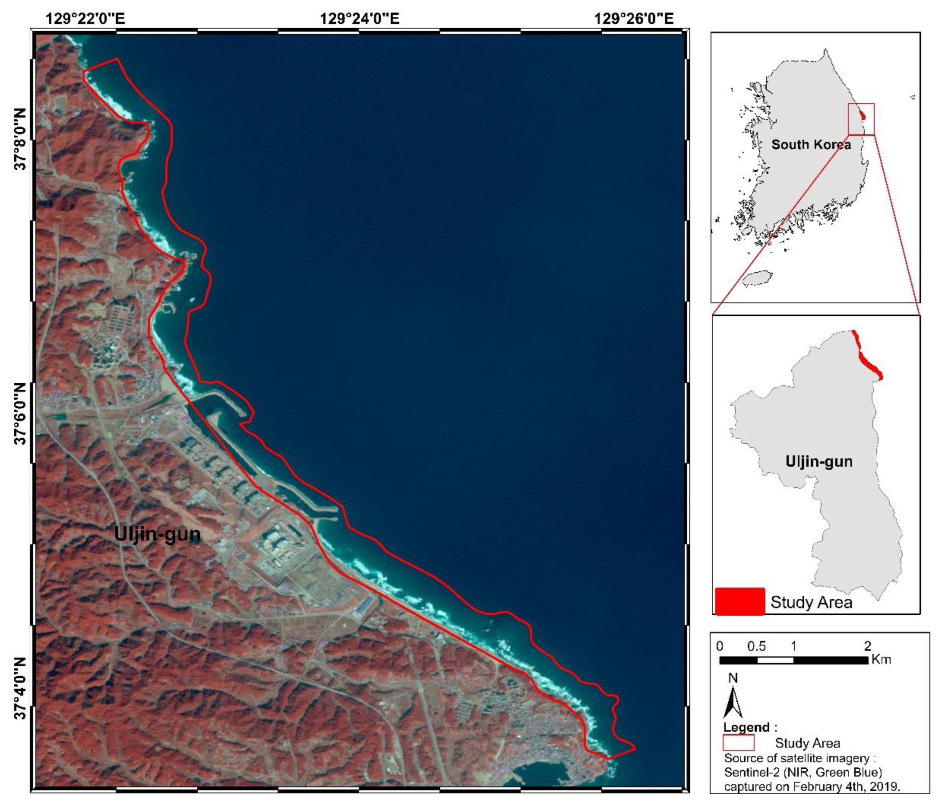
2.1. Study Area

The research area was located around the Korean National Ocean Science Museum, in Uljin-gun, Gyeongsangbuk-do, on the eastern coast of South Korea which was shown in Figure 1. The study was conducted in the coldest season of the year. The total area of study was 480 ha. This study used areas in which water depths were as much as 10 m below mean sea level (MSL), as determined by the Korea Hydrographic and Oceanographic Agency. The studied species of seagrass along Uljin–-gun is a Zostera caulescens, a seagrass species endemic to Northeastern Asia [35].

2.2. Satellite Data

In this research, GeoEye-1, Sentinel-2 MSI level 1C, and Landsat-8 OLI satellite images were selected. The GeoEye-1 satellite produces images with a spatial resolution of 2.0 m for multispectral bands. Several spectral bands were applied in this study, including blue (0.45–0.51 μm), green (0.51–0.58 μm), red (0.65–0.69 μm), and NIR (0.78–0.92 μm), at a quantization level of 11 bits per pixel in each band. The acquisition data for GeoEye-1 were recorded on 13 February 2019.

Sentinel-2 Multi Spectral Instrument (MSI) level 1C (L1C) imaging was used in this study. In cartographic geometry, L1C products have been corrected using at the top of atmosphere (ToA) satellite reflectance data. The images have spectral bands. The Sentinel 2 satellite imagery data from 4 February 2019 were selected. This study used images with spatial resolutions of 10 m, which consisted of three visible bands and an NIR band, which was needed for image corrections.

The satellite imagery of Landsat-8 OLI Level 1 used data path/row 114-34 with 30 m resolution for multispectral bands. The spectral bands used in this study included blue (0.452–0.512 μm), green (0.533–0.590 μm), red (0.636–0.673 μm), and NIR (0.851–0.879 μm). The Landsat-8 OLI data were recorded on 22 January 2019.

2.3. Image Processing

Satellite imagery data for identifying benthic habitats should be radiometrically corrected to remove any disturbances generated by the environment. The classification accuracy of satellite images may be greatly improved by utilizing corrected images, which contain atmospheric, sunglint, and water column corrections.

In this study, we used ACOLITE to perform atmospheric corrections on Landsat-8, Sentinel-2, and GeoEye-1 imagery. Each image consists of blue, green, red, and NIR bands, and all of them were atmospherically corrected. The exploration of underwater radiances in the visible region of the ocean requires the use of atmospheric correction methods for multichannel remote sensing imagery. The ACOLITE atmospheric correction technique has the lowest relative and absolute error values, compared to the existing L2-WFR, POLYMER, C2RCC, SeaDAS and SeaDAS-ALT [36]. Therefore, this atmospheric correction algorithm was used in this study. ACOLITE supports sensors from a variety of satellites, including Landsat 5, 7, 8, Sentinel 2, 3, PlanetScope, and WorldView, with atmospheric correction performed using Dark Spectrum Fitting [23,36,37,38,39]. ACOLITE also works on the basis of an input image, and does not require external inputs, such as aerosol optical thickness (${\tau }_a$) estimates or measurements (such as FLAASH), subject to meeting two conditions: the atmosphere is constant and homogeneous within a limited space, and; at least one pixel in the scene or subscene has a surface reflectance (${\rho }_s$) close to zero, so that the atmospheric path reflectance (${\rho }_{path}$) can be estimated in at least one band [23]. The parameters used to produce the surface-level reflectance are generated by the composite band. The parameter output used in this study was L2R (Level 2, surface-level reflectances) (${\rho }_s$, rhos_*). For the ACOLITE atmospheric corrector method, there are internal parameters, such as minimum gas transmittance for retrieval of aerosol optical thickness, which were all set to default values.

Sunglint is a significantly greater complication for remote sensing of the sea floor and aquatic characteristics via radiometric correction. The sunglint algorithm in shallow waters was developed by Hedley [25]. Utilizing brightness in a NIR band, this approach is advantageous for removing sunglint from remote sensing imagery [24]. Maintaining a steady baseline brightness and low water luminosity in the NIR, the image was chosen to allow for a variety of pixel luminosity levels. Using all pixels in the area covered, a linear regression is performed between the NIR radiance and the visible band radiance. This technique performs a regression analysis of the NIR and visible band data, using random samples of pixel data to obtain a set of regression slopes. The slope of least squares regression is then used to determine the correlation between the visible band and NIR, and each pixel is adjusted by subtracting the visible band from the NIR radiance’s estimated lowest value. The formula in Equation (1) used for sun glint is shown as follows:

$$R_i^{\prime }=R_i-b_i\left(R_{NIR}-Mi{n}_{NIR}\right)$$

(1)

where $R_i^{\prime }$ is the sunlight-free reflectance; $R_i$ is the reflectance from visible band $i$; $b_i$ is the product of the regression slope; $R_{NIR}$ is the reflectance from the NIR band, and; $Mi{n}_{NIR}$ is the minimum NIR band.

Considering that environmental factors, such as the bottom type, water depth, and water attenuation (which may cause scattering and absorption in the water column), can vary widely, water column adjustment is a major challenge. Many water column algorithms were developed, though, in some cases, algorithms were not available due to the requirement for values for bathymetry and the diffuse attenuation coefficient of the water [27]. Therefore, in this study, the Lyzenga algorithm was selected because it could minimize the water attenuation effect in shallow waters, and did not require additional data [27,40]. Spectral characteristics obtained from the ocean’s surface were utilized to recognize the water column depth through the Lyzenga algorithm [41]. The algorithm was continually enhanced and became extensively adopted as the depth invariant index ($DII$) transformation, which could be employed for conducting ecosystem mapping of shallow waters based on satellite data [42,43,44]. Approaches were established to correct for water column, which stems from absorption and scattering by particles in the water [45]. The technique for identifying benthic habitats has potential advantages, including the development of more than two spectral bands to boost performance, improve researchers’ ability to distinguish between bottom components with similar object spectral reflectances, and expand the functional capability without considering the same coefficient of water attenuation [41]. This approach establishes that the bottom type is the primary factor that affects the constant in the linear relationship between the Lyzenga-converted reflectance values of the various bands. The $DII$ index is defined as an expression between bands $i$ and $j$, as follows in Equation (2):

$$DI{I}_{ij}=\ln \left(L_i\right)-\left[\left(\frac{k_i}{k_j}\right)\ln \left(L_j\right)\right]$$

(2)

where $L_i$ is the reflectance value of band $i$; $L_j$ is the reflectance value of band $j$, and; $k_i$/$k_j$ is the following Equation (3) allowed to determine the slope of the interband conversion:

$$\frac{k_i}{k_j}=a+\sqrt{a^2+1}$$

(3)

where $k_i$/$k_j$ is the ratio of the attenuation coefficient values of bands $i$ and $j$, $a$ is the variable defined in Equation (4)

$$a=\frac{\left({\sigma }_{ii}-{\sigma }_{jj}\right)}{\left(2{\sigma }_{ij}\right)}$$

(4)

where ${\sigma }_{ij}$ is the covariance of bands $i$ and j; ${\sigma }_{ii}$ is the variances of band $i$; and ${\sigma }_{jj}$ is the variance of band j. The following image shows $DII$ corrections applied to the values of the three main band ratios, including blue and green (B1/B2), blue and red (B1/B3), and green and red (B2/B3) data [42]; these bands are factored into the equations.

One type of supervised learning algorithm, known as a support vector machine (SVM), is a non-parametric classifier [46]. The objective of support vector machines (SVMs) is to locate a hyperplane that can divide the input dataset into a fixed number of classes in a way that corresponds to the samples used for training [47]. The elements used to classify the image were divided into four classes: land, seagrass, breaking wave, and others.

Table 1. Classes used in this study for classification.

Category of the Class	Description	Sources
Seagrass	Define the distribution of seagrass habitats.	The in-situ data was obtained from Korea Institute of Ocean Science and Technology (KIOST).
Breaking wave	Define the image that contains sea wave disturbance.
Land	Include port, mixed barren land, natural grasses, field, and other grasses.	Korea Institute of Geoscience and Mineral Resource (KIGAM).
Others	Define the water in the coastal area/ocean water.

describes each category. The closest training values in the training datasets, generally referred to as support vectors, were used to increase the margin between the tested point and the ideal hyperplane. When the size of the margins was maximized, there was an improvement in the classification accuracy [48]. The hyperplane in the decision variables was thus established; the SVM model was then developed for each seagrass using the radial gaussian basis function kernel, with approach C and gamma regarded as the best option due to its greater efficiency [49]. The radial gaussian basis function kernel has better performance than other kernels, with powerful capabilities in remote sensing data processing; it simply needs a few numbers of the parameters to be defined [50]. Support vectors selected the best values for the SVM hyperparameters and employed cross validation, with some of the training pixels being retained. The parameters for the classification process using SVM were selected (shown in

Table 2. The selected input parameters of SVM.

Parameter	Parameter
Kernel type	Gaussian basis function
C values	5792.61
Gamma values	32

), and included Kernel Type, C and Gamma in Kernel Function. The selected kernel type was a radial basis function. The C and Gamma values were used 5792.61 and 32, respectively.

We used the equalize random sampling schema to classify the seagrass [51]. In this method, the samples in each class were divided into training and testing steps. The sampled area was segmented into the seagrass, breaking wave, land, and others classes based on two methods. Table 2 shows the definition of each class, which were used as references for dividing the classes for training and testing purposes. From the entire study, the 3737 pixels were selected as references for training, and 1604 pixels were selected for testing. The testing points were selected according to the random sampling method within the label distribution, and were balanced. Training and testing data for seagrass were generated using research from the Korea Institute of Ocean Science and Technology (KIOST), while research from the Korea Institute of Geoscience and Mineral Resource was used for the land and others classes; the breaking wave class data were generated by satellite images. The classified image was then tested to estimate overall accuracy. The accuracy of classification was determined using the method of the percentage of pixels correctly allocated, which is evaluated using the overall accuracy of the classification. Accuracy for a target class is the percentage appropriately labeled to the total number of pixels in that class. We used the matrix’s column and row allocation to define two types of accuracy; these methods are called user’s and producer’s accuracy. Nevertheless, they do not account for agreements across data sets that could be attributed to random chance. The kappa coefficient approach was used to assess the consistency of the output maps by measuring the agreement, based on the actual agreement in the confusion matrix and the chance agreement.

3. Results

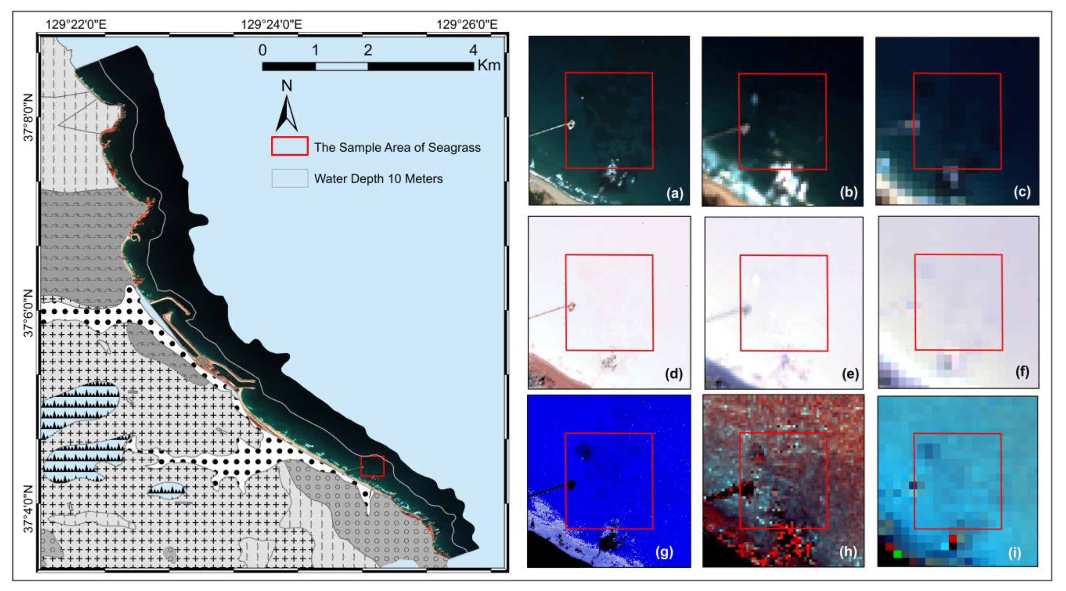
3.1. Atmospheric Correction, Sunglint and Water Column Correction

The first pre-processing steps involve transforming the digital number to the top of atmosphere reflectance. The top of the atmosphere becomes the surface level reflectance. The comparisons due to corrections variations are shown by standard deviation in

Table 3. Comparison of the corrected images by standard deviation values.

	GeoEye-1	Sentinel-2	Landsat-8 OLI
Before correction	5.5	4	9.5
After atmospheric correction	0.000976	0.000603	0.000534
After sunglint correction	0.000276	0.000604	0.000548
After Lyzenga correction	0.189	0.024	0.015

.

The next pre-classification step focuses on removing the effects of sun glint. We used the Hedley algorithm to mitigate the effects of sunglint. The process of sunglint correction required the product of the regression slope. After sunglint processing, the Lyzenga algorithm was applied. Figure 2 presents a comparison of the corrected images from GeoEye-1, Sentinel-2, and Landsat-8. The figure in the red box shows one of the areas in which seagrass habitats lived.

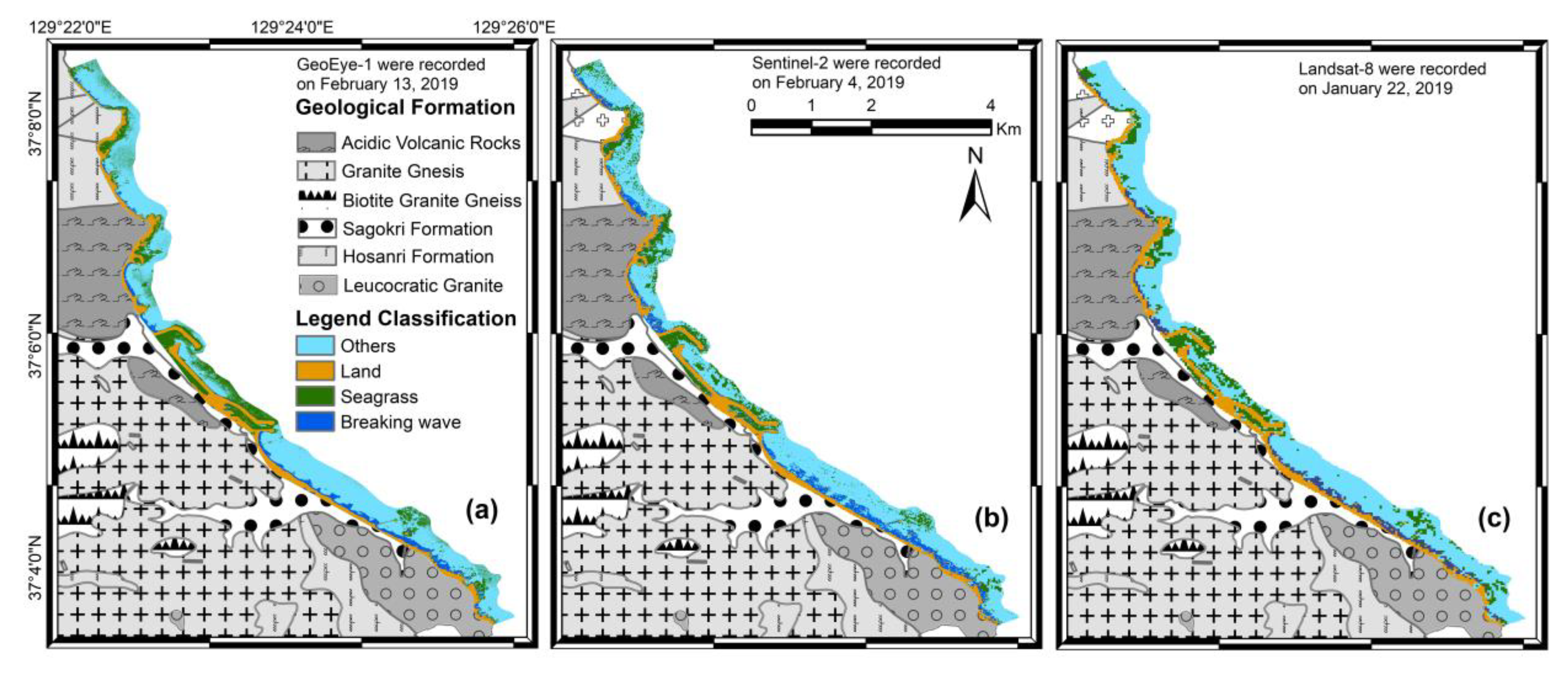
3.2. Image Classification

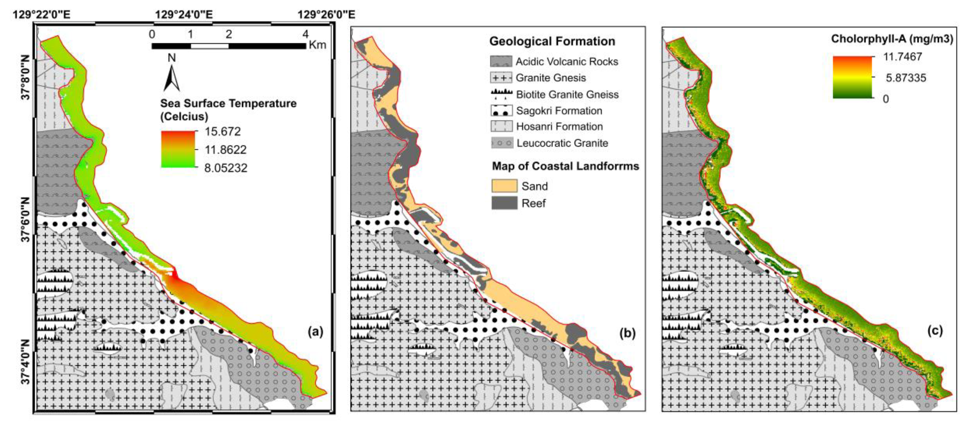
The results of this study provide three models for seagrass distribution along the Uljin-gun area, including mapping of seagrass using GeoEye-1, Sentinel-2, and Landsat-8. The results of the classification images are shown in Figure 3. The green color represented seagrass, the soft blue color represented the others class in waters within $\le$10 m, the blue color represented the breaking wave, and the brown color represented the land area.

The last step is the measurement of overall and kappa accuracy using the equalize random sampling schema. The results of classification without water column correction and with water column correction are shown in Figure 2 and Figure 3. These results should be validated using the error matrices and their related statistics.

Table 4. Confusion matrix for seagrass classification using Geoeye-1.

Class Name	Others	Land	Seagrass	Breaking Wave	Sum	User’s Accuracy
Others	377	0	24	0	401	0.94
Land	2	388	0	9	401	0.96
Seagrass	69	0	332	0	401	0.82
Breaking wave	15	6	0	380	401	0.94
Producer’s Accuracy	0.80	0.98	0.93	0.97
Overall Accuracy	92%
Kappa Accuracy	0.89

,

Table 5. Confusion matrix for seagrass classification using Sentinel-2.

Class Name	Others	Land	Seagrass	Breaking Wave	Sum	User’s Accuracy
Others	358	0	26	17	401	0.89
Land	5	383	0	13	401	0.95
Seagrass	110	0	291	0	401	0.72
Breaking wave	3	4	0	394	401	0.98
Producer’s Accuracy	0.75	0.98	0.91	0.92
Overall Accuracy	88%
Kappa Accuracy	0.85

and

Table 6. Confusion matrix for seagrass classification using Landsat-8 OLI.

Class Name	Others	Land	Seagrass	Breaking Wave	Sum	User’s Accuracy
Others	351	0	43	7	401	0.87
Land	14	368	0	19	401	0.91
Seagrass	93	0	307	1	401	0.76
Breaking wave	51	40	0	310	401	0.77
Producer’s Accuracy	0.64	0.90	0.87	0.91
Overall Accuracy	83%
Kappa Accuracy	0.77

present the producer’s accuracy and user’s accuracy values in each class for GeoEye-1 (Table 4), Sentinel 2 (Table 5), and Landsat 8 (Table 6). The Table 4 shows the confusion matrix for seagrass classification using GeoEye-1, which indicated 7% for the misclassification of seagrass attributed to the others classes. Table 5 explains the confusion matrix for seagrass classification using Sentinel-2, which demonstrated 9% for the misclassification of seagrass attributed to the others classes. Table 6 mentions the confusion matrix for seagrass classification using Landsat, which demonstrated 13% for the misclassification of seagrass attributed to the others and breaking waves classes. However, the SVM classifier for the image with Lyzenga water column correction showed the seagrass influenced by the others class was often confused. It is proposed that the resolution imagery and complex environment lead to a high intra-class variability, making it difficult for the classifier to separate the classes located in the coastal area, especially for classifying the seagrass. The accuracy of classification was indicated by the fact that overall accuracy and kappa accuracy values were 92% and 0.89 for GeoEye-1, 88% and 0.85 for Sentinel-2, and 79% and 0.72 for Landsat-8, respectively. The results of the classification indicate that the implementation of water column correction does not increase accuracy values. Obtaining high accuracy values requires a considerable bathymetric variation and greater water turbidity in the studied areas [27].

4. Discussion

Recently, remote sensing technology has proven to be an effective tool for estimating the distribution of large seagrass habitats on a large scale. The SVM classification methods have been suitable for identifying the seagrass distribution in coastal areas, which was represented with seagrass classes. A previous study applied seagrass classification using Worldview-2 based on a maximum depth of 20 m. Those researchers discovered that SVM results achieved a classification accuracy and kappa coefficient of 72% and 0.61, respectively [52]. Regarding other previous research, seagrass mapping using multispectral satellite imagery was applied by machine learning methods, including SVM [27]. These studies considered water column correction using the Lyzenga algorithm and without water column correction for classifying the seagrass. The accuracy of SVM for the seabed maps of Cabrera was shown by the fact that overall accuracy of image classification was greater without water column corrections than with such corrections; these methods had accuracy rates of 97.9% and 96.9%, respectively.

This study examined four classes for classifying the images:, land, seagrass, breaking wave, and others. The utilization of multispectral satellite imaging for analyzing seagrass is challenging, and extensive processing is needed to reduce distortions caused by the data acquisition process. Adequate preprocessing procedures were used in this work, such as band combination, atmospheric, sunglint, and water column corrections. This study compared estimates of seagrass habitats based on the differences in spatial resolution for satellite imagery of GeoEye-1, Sentinel-2 MSI level 1C, and Landsat-8 OLI, within an area of water depth <10 m. Furthermore, this study picked different spatial resolution for each imaging method: 2m for GeoEye-1, 10 m for Sentinel-2 MSI level 1C, and 30 m for Landsat-8 OLI, respectively. The validation for seagrass mapping is shown to have overall value accuracies of 92%, 88%, and 83% for GeoEye-1, Sentinel 2, and Landsat-8 OLI, respectively. The overall accuracy value was improved by using high spatial resolution images of GeoEye-1, Sentinel-2, and Landsat-8.

We faced several challenges when classifying seagrass in the studied coastal areas. Mapping coastal areas using remote sensing images presents a considerable challenge due to the fluctuations of the tide and other water sources [53]. Misclassifications and the existence of several objects in a pixel were identified as potential factors contributing to misinterpretation. Each class is located in a basic level classification system, with a limited number of classes contains numerous subcategories, resulting in various spectral signatures over the scene [54]. In addition, the spectral identification of seagrass ecosystems using optical data becomes more challenging with expanded depth due to absorption and scattering of light [9], with light penetration depths varying by the wavelengths of sunlight. Six images were successfully used for classifying the seagrass. However, we propose that the fluctuations of the tide along the study area also contributed to the classification results.

This study did not consider bathymetry and water turbidity parameters. Consequently, the effects of the water column could not be described precisely; thus, future research ought to consider bathymetry data and identify the specific bottom types, including sand, pavement, algae, and coral, to further improve classification accuracy. In clearwater, the algorithm developed by Stumpf et al. can generate depths of more than 25 m over variable bottom types; it also demonstrates better stability between regions [55].

Moreover, several studies have shown that seagrass habitats can be affected by sea surface temperature [35] and coastal landforms [30]. The sea surface temperature and coastal landforms along Uljin-gun are illustrated in Figure 4a,b, respectively. These characteristics indicate the oceanographic environments along the coastline of Uljin-gun. The mean sea surface temperature during the coldest month in the 2000s was around 9.8 °C in January [56], and 10.1 °C in February [29]. The sea surface temperature along the Uljin-gun coastline is illustrated in Figure 4a. The majority of the seagrass habitat was in the range of 8.052 °C to 15.672 °C during the winter season, which was generated by the Multi-Channel Sea Surface Temperature-1 (MCSST-1) algorithm using Landsat-8 OLI/TIRS on 4 February 2019. The coastal landforms in the study area, illustrated in Figure 4b, are dominated by sand and reef. Based on the KIOST (Korea Institute of Ocean Science and Technology) data of surface sediment analysis along the coastal area in this study, the size of the average grain of sand in the region was 0.89–2.14 phi. Moreover, based on the data of KIGAM (Korea Institute of Geoscience and Mineral Resource), local reefs were formed from acidic volcanic rocks.

The distribution of seagrass along the coastal area produced variations in chlorophyll concentrations [57]. Chlorophyll content is a relevant indication of sunlight exposure for seagrasses, in addition to being useful for assessing seagrass productivity. Chlorophyll tests were carried out with the objective of identifying the relative contribution of seagrass to the entire meadow productivity, as a possible supply of carbon for consumers [58]. The annual range of marine chlorophyll in Uljin-gun has been reported to be 0.19~10.69 $\mathrm{mg}/{\mathrm{m}}^3$ [59]. The chlorophyll-A along Uljin-gun coastline, as shown in Figure 4c, had a concentration range from 0.034 mg/m³ to 11.746 mg/m³ (generated by Sentinel-2 on 22 January 2019).

5. Conclusions

The mapping seagrass distribution was conducted using imaging data of varying spatial resolutions from the GeoEye-1, Sentinel-2 MSI level 1C, and Landsat-8 OLI satellites. Seagrass distribution mapping using remote sensing technology may be useful for monitoring seagrass on a large scale, particularly when using multispectral band ratios. Band ratio modeling provides an additional band by combining two bands from the visible spectrum in the following products: blue and green (B1/B2), blue and red (B1/B3), and green and red (B2/B3). According to the results, GeoEye-1 was the most effective imaging, method for seagrass habitat data extraction along the coastline of Uljin-gun, with an overall accuracy of 92% and kappa accuracy coefficient of 0.89. In contrast, Sentinel-2 MSI level 1C had an overall accuracy of 88% and a kappa coefficient of 0.85, while Landsat-8 OLI had an overall accuracy of 83% and a Kappa coefficient of 0.77.

References

1. Done, T.J.; Reichelt, R.E. Integrated Coastal Zone and Fisheries Ecosystem Management: Generic Goals and Performance Indices. Ecol. Appl. 1998, 8 (Suppl. S1), S110–S118. [Google Scholar] [CrossRef]
2. Heckbert, S.; Costanza, R.; Poloczanska, E.; Richardson, A. Climate regulation as a service from estuarine and coastal ecosystems. In Treatise on Estuarine and Coastal Science; Elsevier: Amsterdam, The Netherlands, 2011; pp. 199–216. [Google Scholar]
3. Larkum, A.W.D.; Orth, R.J.; Duarte, C.M. Seagrasses: Biology, Ecology and Conservation; Springer: Dordrecht, The Netherlands, 2006. [Google Scholar]
4. den Hartog, C.; Kuo, J. Taxonomy and biogeography of seagrasses. In Seagrasses: Biology, Ecologyand Conservation; Springer: Dordrecht, The Netherlands, 2007; pp. 1–23. [Google Scholar]
5. Zhao, J.; Liu, C.; Li, H.; Liu, J.; Jiang, T.; Yan, D.; Tong, J.; Dong, L. Review on Ecological Response of Aquatic Plants to Balanced Harvesting. Sustainability 2022, 14, 12451. [Google Scholar] [CrossRef]
6. Oreska, M.P.J.; McGlathery, K.J.; Aoki, L.R.; Berger, A.C.; Berg, P.; Mullins, L. The greenhouse gas offset potential from seagrass restoration. Sci. Rep. 2020, 10, 7325. [Google Scholar] [CrossRef] [PubMed]
7. Aben, R.C.; Velthuis, M.; Kazanjian, G.; Frenken, T.; Peeters, E.T.; Van de Waal, D.B.; Hilt, S.; Domis, L.N.D.S.; Lamers, L.P.; Kosten, S. Temperature response of aquatic greenhouse gas emissions differs between dominant plant types. Water Res. 2022, 226, 119251. [Google Scholar] [CrossRef]
8. Phinn, S.; Roelfsema, C.; Kovacs, E.; Canto, R.; Lyons, M.; Saunders, M.; Maxwell, P. Mapping, Monitoring and Modelling Seagrass Using Remote Sensing Techniques. In Seagrasses of Australia; Springer International Publishing: Cham, Switzerland, 2018; pp. 445–487. [Google Scholar]
9. Veettil, B.K.; Ward, R.D.; Lima, M.D.A.C.; Stankovic, M.; Hoai, P.N.; Quang, N.X. Opportunities for seagrass research derived from remote sensing: A review of current methods. Ecol. Indic. 2020, 117, 106560. [Google Scholar] [CrossRef]
10. Dekker, A.; Brando, V.; Anstee, J.; Fyfe, S.; Malthus, T.; Karpouzli, E. Remote sensing of seagrass ecosystems: Use of spaceborne and airborne sensors. In Seagrasses: Biology, Ecologyand Conservation; Springer: Dordrecht, The Netherlands, 2007; pp. 347–359. [Google Scholar]
11. Duffy, J.P.; Pratt, L.; Anderson, K.; Land, P.E.; Shutler, J.D. Spatial assessment of intertidal seagrass meadows using optical imaging systems and a lightweight drone. Estuar. Coast. Shelf Sci. 2018, 200, 169–180. [Google Scholar] [CrossRef]
12. Dierssen, H.M.; Zimmerman, R.C.; Leathers, R.A.; Downes, T.V.; Davis, C.O. Ocean color remote sensing of seagrass and bathymetry in the Bahamas Banks by high-resolution airborne imagery. Limnol. Oceanogr. 2003, 48 Pt 2, 444–455. [Google Scholar] [CrossRef]
13. Paul, M.; Lefebvre, A.; Manca, E.; Amos, C. An acoustic method for the remote measurement of seagrass metrics. Estuar. Coast. Shelf Sci. 2011, 93, 68–79. [Google Scholar] [CrossRef]
14. Bakirman, T.; Gumusay, M.U.; Tuney, I. Mapping of The Seagrass Cover Along the Mediterranean Coast of Turkey Using Landsat 8 OLI Images. In Proceedings of the ISPRS—International Archives of the Photogrammetry, Remote Sensing and Spatial Information Sciences, XXIII ISPRS Congress, Prague, Czech Republic, 12–19 July 2016; Volume XLI-B8, pp. 1103–1105. [Google Scholar]
15. Topouzelis, K.; Makri, D.; Stoupas, N.; Papakonstantinou, A.; Katsanevakis, S. Seagrass mapping in Greek territorial waters using Landsat-8 satellite images. Int. J. Appl. Earth Obs. Geoinf. 2018, 67, 98–113. [Google Scholar] [CrossRef]
16. Ha, N.T.; Manley-Harris, M.; Pham, T.D.; Hawes, I. A Comparative Assessment of Ensemble-Based Machine Learning and Maximum Likelihood Methods for Mapping Seagrass Using Sentinel-2 Imagery in Tauranga Harbor, New Zealand. Remote. Sens. 2020, 12, 355. [Google Scholar] [CrossRef] [Green Version]
17. Traganos, D.; Reinartz, P. Mapping Mediterranean seagrasses with Sentinel-2 imagery. Mar. Pollut. Bull. 2018, 134, 197–209. [Google Scholar] [CrossRef] [PubMed] [Green Version]
18. Pasqualini, V.; Pergent-Martini, C.; Pergent, G.; Agreil, M.; Skoufas, G.; Sourbes, L.; Tsirika, A. Use of SPOT 5 for mapping seagrasses: An application to Posidonia oceanica. Remote. Sens. Environ. 2005, 94, 39–45. [Google Scholar] [CrossRef]
19. Baumstark, R.; Duffey, R.; Pu, R. Mapping seagrass and colonized hard bottom in Springs Coast, Florida using WorldView-2 satellite imagery. Estuar. Coast. Shelf Sci. 2016, 181, 83–92. [Google Scholar] [CrossRef]
20. Su, L.; Huang, Y. Seagrass Resource Assessment Using WorldView-2 Imagery in the Redfish Bay, Texas. J. Mar. Sci. Eng. 2019, 7, 98. [Google Scholar] [CrossRef] [Green Version]
21. Ryan, R.E.; Pagnutti, M. Enhanced absolute and relative radiometric calibration for digital aerial cameras. In Photogrammetric Week’09; Fritch, D., Ed.; Wichtmann Verlag: Heidelberg, Germany, 2009; pp. 81–90. [Google Scholar]
22. Fan, Y.; Li, W.; Chen, N.; Ahn, J.-H.; Park, Y.-J.; Kratzer, S.; Schroeder, T.; Ishizaka, J.; Chang, R.; Stamnes, K. OC-SMART: A machine learning based data analysis platform for satellite ocean color sensors. Remote. Sens. Environ. 2021, 253, 112236. [Google Scholar] [CrossRef]
23. Vanhellemont, Q.; Ruddick, K. Atmospheric correction of metre-scale optical satellite data for inland and coastal water applications. Remote. Sens. Environ. 2018, 216, 586–597. [Google Scholar] [CrossRef]
24. Kay, S.; Hedley, J.D.; Lavender, S. Sun Glint Correction of High and Low Spatial Resolution Images of Aquatic Scenes: A Review of Methods for Visible and Near-Infrared Wavelengths. Remote. Sens. 2009, 1, 697–730. [Google Scholar] [CrossRef] [Green Version]
25. Hedley, J.D.; Harborne, A.R.; Mumby, P.J. Technical note: Simple and robust removal of sun glint for mapping shallow-water benthos. Int. J. Remote Sens. 2005, 26, 2107–2112. [Google Scholar] [CrossRef]
26. Traganos, D.; Aggarwal, B.; Poursanidis, D.; Topouzelis, K.; Chrysoulakis, N.; Reinartz, P. Towards Global-Scale Seagrass Mapping and Monitoring Using Sentinel-2 on Google Earth Engine: The Case Study of the Aegean and Ionian Seas. Remote. Sens. 2018, 10, 1227. [Google Scholar] [CrossRef] [Green Version]
27. Mederos-Barrera, A.; Marcello, J.; Eugenio, F.; Hernández, E. Seagrass mapping using high resolution multispectral satellite imagery: A comparison of water column correction models. Int. J. Appl. Earth Obs. Geoinf. 2022, 113, 102990. [Google Scholar] [CrossRef]
28. Chandra, M.A.; Bedi, S.S. Survey on SVM and their application in image classification. Int. J. Inf. Technol. 2021, 13, 1–11. [Google Scholar] [CrossRef]
29. Kim, J.B.; Park, J.-I.; Jung, C.-S.; Lee, P.-Y.; Lee, K.-S. Distributional range extension of the seagrass Halophila nipponica into coastal waters off the Korean peninsula. Aquat. Bot. 2009, 90, 269–272. [Google Scholar] [CrossRef]
30. Lee, K.S.; Kim, S.H.; Kim, Y.K. Current Status of Seagrass Habitat in Korea. In The Wetland Book; Springer: Dordrecht, The Netherlands, 2018; pp. 1589–1596. [Google Scholar]
31. Short, F.; Carruthers, T.; Dennison, W.; Waycott, M. Global seagrass distribution and diversity: A bioregional model. J. Exp. Mar. Biol. Ecol. 2007, 350, 3–20. [Google Scholar] [CrossRef]
32. Hyun, J.-H.; Choi, K.-S.; Lee, K.-S.; Lee, S.H.; Kim, Y.K.; Kang, C.-K. Climate Change and Anthropogenic Impact Around the Korean Coastal Ecosystems: Korean Long-term Marine Ecological Research (K-LTMER). Estuaries Coasts 2020, 43, 441–448. [Google Scholar] [CrossRef] [Green Version]
33. Kim, M.; Qin, L.-Z.; Kim, S.H.; Song, H.-J.; Kim, Y.K.; Lee, K.-S. Influence of Water Temperature Anomalies on the Growth of Zostera marina Plants Held Under High and Low Irradiance Levels. Estuaries Coasts 2020, 43, 463–476. [Google Scholar] [CrossRef]
34. Qin, L.-Z.; Kim, S.H.; Song, H.-J.; Suonan, Z.; Kim, H.; Kwon, O.; Lee, K.-S. Influence of Regional Water Temperature Variability on the Flowering Phenology and Sexual Reproduction of the Seagrass Zostera marina in Korean Coastal Waters. Estuaries Coasts 2020, 43, 449–462. [Google Scholar] [CrossRef]
35. Kim, J.-H.; Park, S.H.; Kim, Y.K.; Kim, S.H.; Park, J.-I.; Lee, K.-S. Seasonal growth dynamics of the seagrass Zostera caulescens on the eastern coast of Korea. Ocean Sci. J. 2014, 49, 391–402. [Google Scholar] [CrossRef]
36. Vanhellemont, Q.; Ruddick, K. Atmospheric correction of Sentinel-3/OLCI data for mapping of suspended particulate matter and chlorophyll-a concentration in Belgian turbid coastal waters. Remote Sens. Environ. 2021, 256, 112284. [Google Scholar] [CrossRef]
37. Vanhellemont, Q. Adaptation of the dark spectrum fitting atmospheric correction for aquatic applications of the Landsat and Sentinel-2 archives. Remote. Sens. Environ. 2019, 225, 175–192. [Google Scholar] [CrossRef]
38. Vanhellemont, Q. Daily metre-scale mapping of water turbidity using CubeSat imagery. Opt. Express 2019, 27, A1372–A1399. [Google Scholar] [CrossRef]
39. Vanhellemont, Q. Sensitivity analysis of the dark spectrum fitting atmospheric correction for metre- and decametre-scale satellite imagery using autonomous hyperspectral radiometry. Opt. Express 2020, 28, 29948–29965. [Google Scholar] [CrossRef] [PubMed]
40. Kutser, T.; Hedley, J.; Giardino, C.; Roelfsema, C.; Brando, V.E. Remote sensing of shallow waters—A 50 year retrospective and future directions. Remote. Sens. Environ. 2020, 240, 111619. [Google Scholar] [CrossRef]
41. Lyzenga, D.R. Passive remote sensing techniques for mapping water depth and bottom features. Appl. Opt. 1978, 17, 379–383. [Google Scholar] [CrossRef] [PubMed]
42. Siregar, V.P.; Agus, S.B.; Subarno, T.; Prabowo, N.W. Mapping shallow waters habitats using OBIA by applying several approaches of depth invariant index in North Kepulauan Seribu. IOP Conf. Ser. Earth Environ. Sci. 2018, 149, 012052. [Google Scholar] [CrossRef]
43. Aljahdali, M.H.; Elhag, M. Calibration of the depth invariant algorithm to monitor the tidal action of Rabigh City at the Red Sea Coast, Saudi Arabia. Open Geosciences. 2020, 12, 1666–16678. [Google Scholar] [CrossRef]
44. Inamdar, D.; Rowan, G.S.; Kalacska, M.; Arroyo-Mora, J.P. Water column compensation workflow for hyperspectral imaging data. MethodsX 2022, 9, 101601. [Google Scholar] [CrossRef]
45. Manuputty, A.; Gaol, J.L.; Agus, S.B.; Nurjaya, I.W. The utilization of Depth Invariant Index and Principle Component Analysis for mapping seagrass ecosystem of Kotok Island and Karang Bongkok, Indonesia. IOP Conf. Ser. Earth Environ. Sci. 2017, 54, 12083. [Google Scholar] [CrossRef] [Green Version]
46. Cortes, C.; Vapnik, V. Support-vector networks. Mach Learn. 1995, 20, 273–297. [Google Scholar] [CrossRef]
47. Kavzoglu, T.; Colkesen, I. A kernel functions analysis for support vector machines for land cover classification. Int. J. Appl. Earth Obs. Geoinf. 2009, 11, 352–359. [Google Scholar] [CrossRef]
48. Lenz, B.; Barak, B. Data Mining and Support Vector Regression Machine Learning in Semiconductor Manufacturing to Improve Virtual Metrology. In Proceedings of the 2013 46th Hawaii International Conference on System Sciences, IEEE, Wailea, HI, USA, 7–10 January 2013; pp. 3447–3456. [Google Scholar]
49. Baek, W.-K.; Jung, H.-S. Performance Comparison of Oil Spill and Ship Classification from X-Band Dual- and Single-Polarized SAR Image Using Support Vector Machine, Random Forest, and Deep Neural Network. Remote. Sens. 2021, 13, 3203. [Google Scholar] [CrossRef]
50. Tzeng, Y.-C.; Fan, K.-T.; Chen, K.-S. An Adaptive Thresholding Multiple Classifiers System for Remote Sensing Image Classification. Photogramm. Eng. Remote. Sens. 2009, 75, 679–687. [Google Scholar] [CrossRef]
51. Congalton, R.G. A review of assessing the accuracy of classifications of remotely sensed data. Remote Sens. Environ. 1991, 37, 35–46. [Google Scholar] [CrossRef]
52. Bakirman, T.; Gumusay, M.U. Assessment of Machine Learning Methods for Seagrass Classification in the Mediterranean. Balt. J. Mod. Comput. 2020, 8, 315–326. [Google Scholar] [CrossRef]
53. Gallant, A.L. The Challenges of Remote Monitoring of Wetlands. Remote. Sens. 2015, 7, 10938–10950. [Google Scholar] [CrossRef] [Green Version]
54. Zhang, C.; Selch, D.; Xie, Z.; Roberts, C.; Cooper, H.; Chen, G. Object-based benthic habitat mapping in the Florida Keys from hyperspectral imagery. Estuar. Coast. Shelf Sci. 2013, 134, 88–97. [Google Scholar] [CrossRef]
55. Stumpf, R.P.; Holderied, K.; Sinclair, M. Determination of water depth with high-resolution satellite imagery over variable bottom types. Limnol. Oceanogr. 2003, 48 Pt 2, 547–556. [Google Scholar] [CrossRef]
56. Park, J.-I.; Kim, J.-H.; Park, S.H. Growth dynamics of the deep-water Asian eelgrass, Zostera asiatica, in the eastern coastal waters of Korea. Ocean Sci. J. 2016, 51, 613–625. [Google Scholar] [CrossRef]
57. Halasan, L.; Dy, D. Chlorophyll content of Thalassia hemprichii (Ehrenberg) Ascherson leaves in some coastal areas of Cebu Island, Central Philippines. Ann. Trop. Res. 2018, 40, 35–44. [Google Scholar] [CrossRef] [Green Version]
58. Dawes, C.J. Marine Botany, 2nd ed.; John Wiley & Sons, Inc.: New York, NY, USA, 1998. [Google Scholar]
59. Yoon, Y.H. Spatio-temporal Fluctuation of Phytoplankton Size Fractionation in the Uljin Marine Ranching Area (UMRA), East Sea of Korea. Korean J. Environ. Biol. 2016, 34, 151–160. [Google Scholar] [CrossRef]
Figure 1. Area of this study, indicated by a red line.
Jmse 11 00701 g001
Figure 2. Impact of atmospheric, sun-glint, and water column corrections on the Uljin–gun area: (a) atmospheric correction of GeoEye-1, (b) atmospheric correction of Sentinel-2, (c) atmospheric correction of Landsat-8, (d) sun-glint corrections of GeoEye-1, (e) sunglint corrections of Sentinel-2, (f) sunglint corrections of Landsat-8, (g) water column corrections of GeoEye-1 (h) water column corrections of Sentinel-2, and (i) water column corrections of Landsat-8.
Jmse 11 00701 g002
Figure 3. The classification results of the SVM methods for seagrass distribution in the Uljin-gun using (a) GeoEye-1 (b) Sentinel-2 (c) Landsat-8 satellite, with Lyzenga water column correction.
Jmse 11 00701 g003
Figure 4. Oceanography conditions mapping (a) sea surface temperature distribution (b) map of coastal landforms along Uljin-gun (c) chlorophyll-a distribution.
Jmse 11 00701 g004