Deriving Coastal Shallow Bathymetry from Sentinel 2-, Aircraft- and UAV-Derived Orthophotos: A Case Study in Ligurian Marinas

Abstract

Bathymetric surveys of shallow waters are increasingly necessary for navigational safety and environmental studies. In situ surveys with floating acoustic sensors allow the collection of high-accuracy bathymetric data. However, such surveys are often unfeasible in very shallow waters in addition to being expensive and requiring specific sectorial skills for the acquisition and processing of raw data. The increasing availability of optical images from Uncrewed Aerial Vehicles, aircrafts and satellites allows for bathymetric reconstruction from images thanks to the application of state-of-the-art algorithms. In this paper, we illustrate a bathymetric reconstruction procedure involving the classification of the seabed, the calibration of the algorithm for each class and the subsequent validation. We applied this procedure to high-resolution, UAV-derived orthophotos, aircraft orthophotos and Sentinel-2 Level-2A images of two marinas along the western Ligurian coastline in the Mediterranean Sea and validated the results with bathymetric data derived from echo-sounder surveys. Our findings showed that the aircraft-derived bathymetry is generally more accurate than the UAV-derived and Sentinel-2 bathymetry in all analyzed scenarios due to the smooth color of the aircraft orthophotos and their ability to reproduce the seafloor with a considerable level of detail.

1. Introduction

Coastal zones are rapidly changing environments due to anthropogenic activity (e.g., settlements and tourist activities) and climate change and its effects (e.g., storms, floods, rising sea level and coastal erosion) [1]. The effects related to extreme events involve several sectors of the coastal marine compartment, especially those that are densely populated and man-made as these are particularly sensitive to disruptive events. For example, storms and surges can potentially damage infrastructure and buildings. On the Ligurian coast (Italy), the last five years have seen two particularly intense events, the Vaia storm (2018) and the Alex storm (2020), which caused severe damage to property and people [2,3]. In addition, many coastal states are moving toward an integrated plan to develop and maximize each nation’s Blue Economy, proposing strategies for the exploitation, conservation and regeneration of the marine environment with a sustainable development approach to coastal resources [4]. The key Blue Economy report [5] from the Organisation for Economic Co-operation and Development (OECD) highlights offshore wind, fish processing, industrial marine aquaculture, port activities and industrial capture fisheries as the top five growth sectors. There is no doubt that mapping shallow water bathymetry in coastal and near-shore areas is crucial to decision makers, entrepreneurs, hydrographers and scientists who need to better understand this dynamic environment and study a wide range of coastal applications. Accurate and up-to-date bathymetry information is required for navigation, dredging planning, environmental management, aquaculture and benthic habitat mapping [6].

Bathymetric surveying based on acoustic sensors on boats, using Single Beam Echo-Sounder (SBES) and Multi-Beam Echo-Sounder (MBES) methodologies, is a well-established technique that allows for high accuracy to be achieved [7,8]. However, at the same time, it is an expensive technique requiring careful calibration of the installed sensors and long processing times of the acquired data, and it can be difficult to be applied in very shallow water or inaccessible coastal areas [9,10]. Equally expensive [11] are bathymetric surveys based on Laser Imaging Detection and Ranging (LIDaR), which, in shallow water, may suffer from transient water turbidity [12] and are affected by the difficulty of separating surface, water column and bottom reflections [13].

Remote Sensing (RS)-based methods seek to overcome these limitations. According to a recent overview [14,15], optical images, coming from Uncrewed Aerial Vehicles (UAV), aircraft or satellites, are used to derive bathymetry in shallow water; synthetic aperture radar (SAR) sensors are considered useful for intermediate water depths [16,17,18]; and radar altimeters are usually used for deep and open oceans and have low resolution [19,20,21].

The increasing availability of optical images, combined with in situ measurements, allows the application of optical remote-derived bathymetry (RDB), i.e., the derivation of the depths of seas, lakes or rivers, from RS optical images. This can be achieved with state-of-the-art analytical, semi-analytical or empirical methods [22] or, more recently, with machine learning techniques [23]. Examples of newly developed algorithms include S2Shores (Satellite to Shores) [24] which inverts coastal bathymetry from wave kinematics based on the linear dispersion relation, and the combination of a new stereo triangulation method and spectral inversion models [25].

Analytical or semi-analytical implementation is based on the transmission of light in water and requires as input a set of parameters related to the properties of the atmosphere, water column and bottom material [15]. On the other hand, the empirical implementation only requires in situ sampled points. The detectable depth is usually limited to shallow waters, and the achievable accuracy in surveying decreases with the increase in water depth. Other influencing factors include water turbidity and seabed materials, as well as image properties [26].

Two widely adopted empirical models for bathymetry computation from optical RS images based on optical band ratio transformations are defined by Lyzenga [27] and Stumpf [28]. In particular, the latter proposes a solution using the ratio of reflectances that can be applied to low-albedo multispectral images (in this case, IKONOS satellite images) for deriving bathymetry.

A comparison of analytical and empirical methodologies to obtain shallow-water bathymetry in Australian and Caribbean coastal environments is provided by Dekker et al. [29]. They focus on RS hyperspectral, radiometrically calibrated reflectances, showing that all the proposed methods provide “moderately accurate retrievals of bathymetry, water column inherent optical properties, and benthic reflectance in waters less than 13 m deep with homogeneous to heterogeneous benthic/substrate covers”. Klonowski et al. [30] describe a semi-analytical method for the quantitative assessment of the bathymetry and the sea bottom cover in shallow waters from hyperspectral imagery, employing a “shallow water reflectance model, which accounts for the water column absorption and backscattering, water depth and substrate reflectance”.

The results obtained in the various optical RDB studies strongly depend on the type and quality of available images, which can be classified into three categories, according to the three platforms that produce them: Uncrewed Aerial Vehicles (UAV), aircraft and satellite.

With the increasing availability of UAV imagery datasets, bathymetry acquisition based on RGB images is becoming “efficient and low-cost when compared to sound-based or LiDAR methods” (ref. [25] pp. 12–13). These platforms also allow deriving bathymetric measurements from videos [31]. Recent RDB studies applying empirical algorithms on UAV-produced multispectral imaging [32], employing extensions of the logarithmic band-ratio technique, show relatively good results with up to 40 cm of vertical errors [33].

Aircraft orthophotos are an additional source of data for bathymetric derivation [29,30]. Mandlburger et al. [34] propose a method for bathymetry derivation from multispectral aircraft images using a deep neural network based on concurrently acquired laser bathymetry data used for training, testing and validation. However, aircraft orthophotos are very sensitive to the problem of surface reflection due to effects of waves and wind on the surface of the water body [35].

Aircraft and UAV orthophotos have very high resolutions but usually cover relatively limited areas compared with satellite-based acquisitions, which also provide broader temporal coverage. The combined use of different types of orthophotos to derive the bathymetry of a location is therefore useful to balance the different characteristics of the input images, as shown in Rossi et al. [33], who employed UAV-derived orthomosaic and WorldView-2 satellite images, combined with MBES data for model calibration.

Multispectral satellite images, at various resolutions, are widely used to derive bathymetry in coastal areas using both linear [36,37,38] and polynomial [39] empirical models. While some studies [33,38,40] use high-resolution satellite imagery (e.g., WORLDVIEW-2, RapidEye) provided for a fee, most rely on open data imagery provided by space programs such as NASA’s Landsat and the European Copernicus [6,9,11,12,41,42,43,44,45]. Caballero et al. [6] analyzed the performance of the S-2-derived bathymetry method with Sentinel-2A and 2B (S-2) for bathymetry recovery in near-shore waters with certain turbidities. Yang et al. [43] used S-2 images to empirically derive the depth of high mountain lakes through machine learning models. The mean absolute error (MAE) and root squared error (RMSE) obtained were 0.54 and 0.89 m, respectively. However, the accuracy of this type of derivation is very sensitive to the presence of a highly heterogeneous seabed cover; the approach is, therefore, dependent on location and time [36].

Among the literature reviewed, some researchers derive bathymetry from optical images acquired from different platforms [6,12,25,33,36,45], usually comparing the results obtained with other data sources, such as echosounders or LIDaR. Some of them [36,45] compare the use of images derived from different satellite missions, such as Sentinel-2 and Landsat-8. Rossi et al. [33] compare the results derived using UAV and very high spatial resolution satellite image from WorldView-2 mission. None of them compare UAV, aircraft and S-2 images in the same area, as proposed in the present paper. In addition, note that few studies address the problem of seafloor classification contextually to RDB regression procedure [29,30,36,40,44], while most of the studies apply RDB to areas with uniform seafloor, where the classification is not needed.

The paper focuses on the bathymetry of shallow water in marinas, i.e., small touristic port areas, which are susceptible to rapid morphological changes of the seabed, to the hydrodynamics derived from wave and marine currents, particularly frequent with the increasing number of high-energy events such as sea storms [3]. Sediment deposition at the entrance to the harbor affects the usability of marinas by larger vessels, while erosion near the breakwaters, which protect the harbor, could compromise its stability. For this reason, recurring bathymetric surveys are often necessary. Hence, a procedure for a quick, not-so-accurate but inexpensive assessment of the state of the seabed and its evolution could be useful to verify the need for a detailed survey, dredging or nourishment and also to support expeditious REA (Rapid Environmental Assessment) surveys in coastal shallow marinas.

The paper presents the potential and limitations of RDB computation by analyzing and comparing the results achieved from UAV, aircraft and S-2 orthophotos, focusing on seabed classification and the coherence of different resolutions of images and bathymetry. The analysis of bathymetric depths was applied to two marina areas of the Mediterranean Sea, on the western Ligurian coast, Italy, using in situ data for calibration and validation of the Stumpf method.

2. Materials and Methods

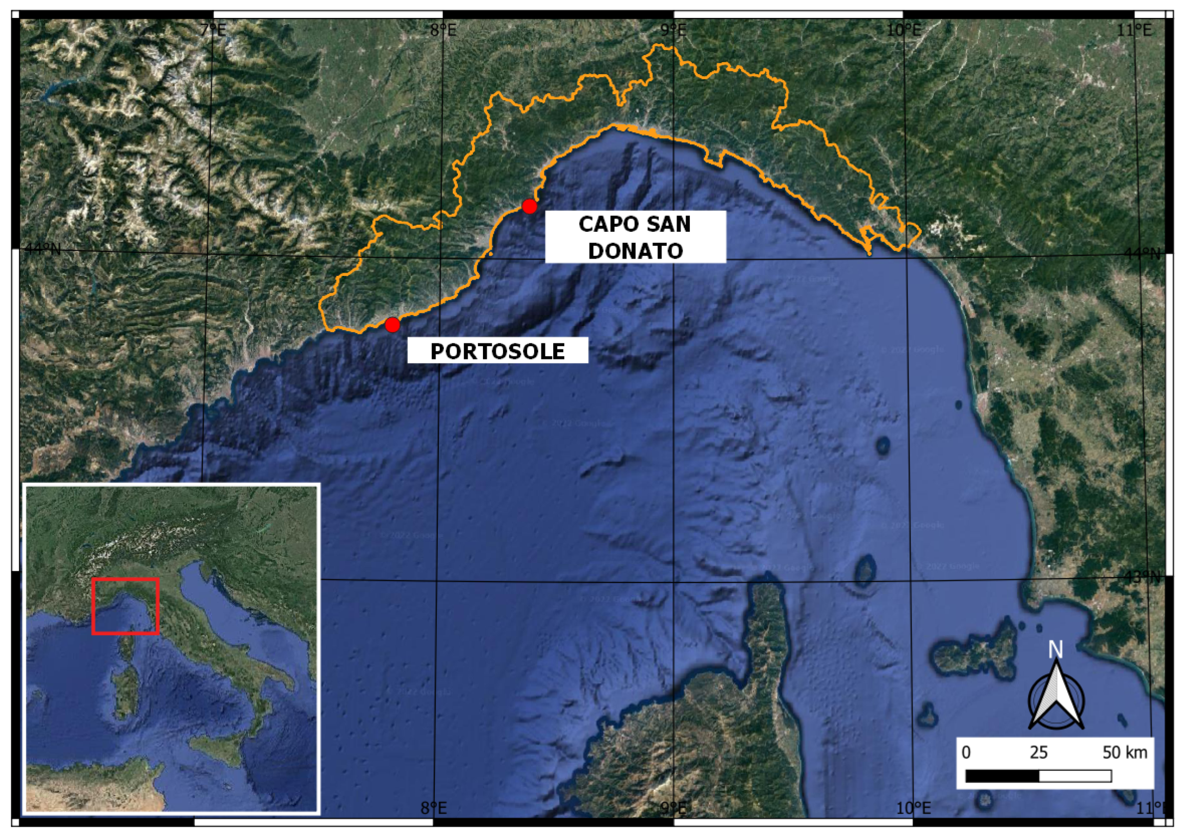
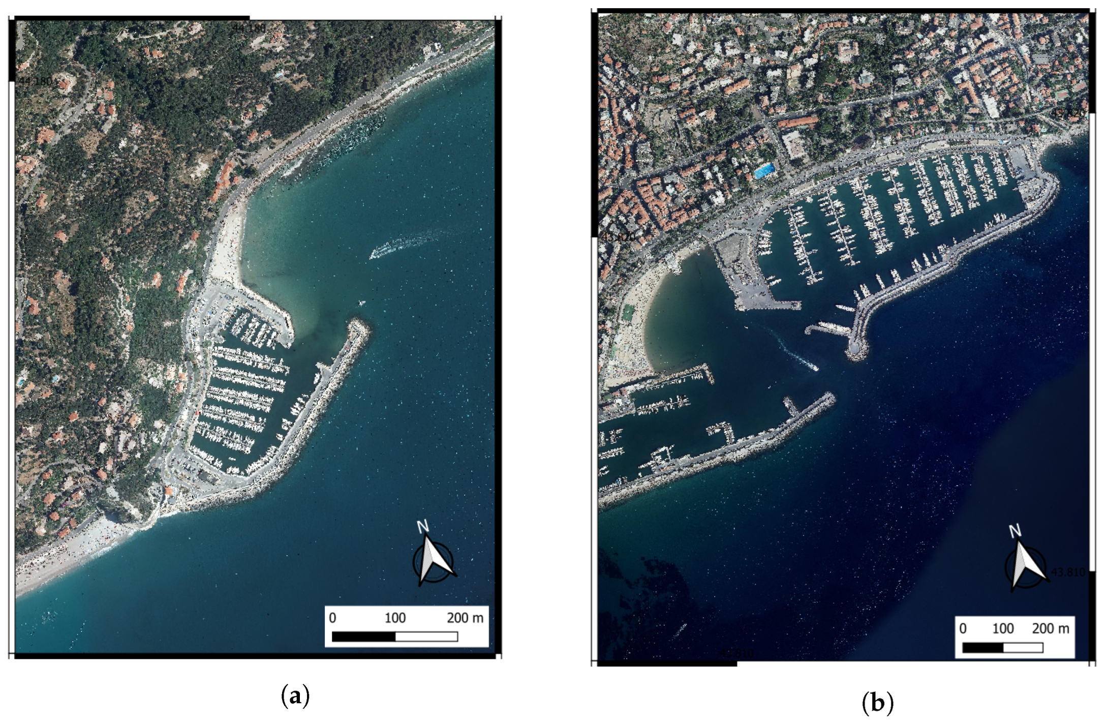
This section describes the two Areas Of Interest (AOIs), the different datasets involved in this study and the methods used for the computation of the RDB.

2.1. Study Areas

The computation and analysis of bathymetric depths considered two AOIs characterized by shallow waters near two marinas on the western Ligurian coast in Italy: Capo San Donato marina in Finale Ligure (${44}^{\circ }{24}^{\prime }{93}^{″}$N–${08}^{\circ }{50}^{\prime }{48}^{″}$E) and Portosole marina in Sanremo (${43}^{\circ }{48}^{\prime }{98}^{″}$N–${07}^{\circ }{47}^{\prime }{24}^{″}$E), depicted in Figure 1 and Figure 2.

The AOI of Capo San Donato (Figure 2a) is external to the entrance channel of the marina, located on the eastern side and exposed to the northeast. The marina has an area of about 500 × 300 m² and the depth at the entrance is not greater than 5 m, where the seafloor is mostly sandy and flat.

The Portosole marina (Figure 2b) is larger and capable of accommodating longer vessels with greater draught, as the depth in the port area ranges from −7 m to −2.5 m. The access to the port is in the central part of the breakwater, facing southwest. Here, the attention is focused on the beach adjacent to the marina on the east side and on the area outside the breakwater, which extends for about 850 m. The breakwater is a rubble mound breakwater constituted of blocks of about 3 × 3 m in size for the base and 2 × 2 m for the coarse-shaped upper part. The seabed facing it is mostly sandy with the presence of Posidonia Oceanica meadows and spots of the natural and artificial rocky bottom. The seafloor is locally steep near the beach slope and the breakwater, with a depth ranging between −12 m and 0 m.

2.2. Data Selection

The images used in the present study consist of three orthophotos for each AOI, derived by the different platforms, at different resolutions: UAV, aircraft and S-2. Moreover, in situ SBES and MBES data were used as reference bathymetry, i.e., Ground truth Points (GPs), for calibration and validation of the RDB model.

Table 1. Dataset description: spatial resolution and acquisition dates of orthophotos and GPs for Capo San Donato.

	Data	Spatial Resolution	Acquisition Date	Flight/Orbital Altitude
Ortophotos	UAV	0.02 m	April 2019	30 m
	Aircraft	0.2 m	Summer 2019	3400 m
	S-2	10 m	April 2019	800 km
GPs	SBES	10 m	April 2019

and

Table 2. Dataset description: spatial resolution and acquisition dates of orthophotos and GPs for Portosole.

	Data	Spatial Resolution	Acquisition Date	Flight/Orbital Altitude
Ortophotos	UAV	0.02 m	February 2019	35 m
	Aircraft	0.2 m	Summer 2019	3400 m
	S-2	10 m	February 2019	800 km
GPs	MBES	0.02 m	February 2019

summarize the spatial resolution and the acquisition time of the images and of the in situ data, respectively, for Capo San Donato and Portosole.

Figure 3 and Figure 4 depict the three orthophotos used for the AOI of Capo San Donato and Portosole, respectively. The difference in spatial resolution, which results different levels of detail, between UAV and aircraft images compared to satellite images is evident, especially in the shallow area.

2.2.1. UAV-Derived Orthophotos

Capo San Donato. The UAV-derived orthophoto related to Capo San Donato covers an area of 200 × 300 m². The UAV survey was conducted 30 m Above Ground Level (AGL) with a DJI Mini, by Maifredi Geological Associated Studio. The orthophoto was produced using the photogrammetric suite Agisoft LLC (St. Petersburg, Russia) Metashape© [46] and is available in the Rome40 datum, in Gauss–Boaga carthographic projection (EPSG code: 3003), at a spatial ground resolution of 1.3 cm. From Figure 3a, one can note the shadow effects in the UAV image caused by the presence of the hill on the western side of the AOI, which alters the color of the water both outside and inside the marina. For this reason, the RDB workflow was not applied to the shaded area for any platform.

Portosole. The UAV-derived orthophoto related to Portosole covers an area of 400 × 800 m². The UAV survey was conducted at 35 m AGL with a DJI Phantom 4 Pro, resulting in a Ground Sample Distance (GSD) of 7.2 mm. The orthophoto was produced by Drafinsub Srl. using the photogrammetric suite Agisoft Metashape© [46], framed in the ETRS89 reference system and projected in the Universal Transverse Mercator (UTM) zone 32N (EPSG code: 32632), with a 2 cm pixel resolution.

2.2.2. Aircraft Orthophotos

The aircraft orthophoto is derived from the mosaicking of digitized, orthorectified and georeferenced aero-photogrammetric images.

The aircraft RGB orthophoto relative to 2019, covering the entire Liguria Region territory (Figure 2b), is visible and accessible through the Open Geospatial Consortium (OGC) Web Map Service (WMS) on the Liguria Region geoportal [47]. The image of the AOI was downloaded thanks to customized credentials given to the university for research and teaching purposes.1 The used datum is ETRS89, projected UTM 32N zone (EPSG code: 25832), and the geometrical resolution is 0.2 m.

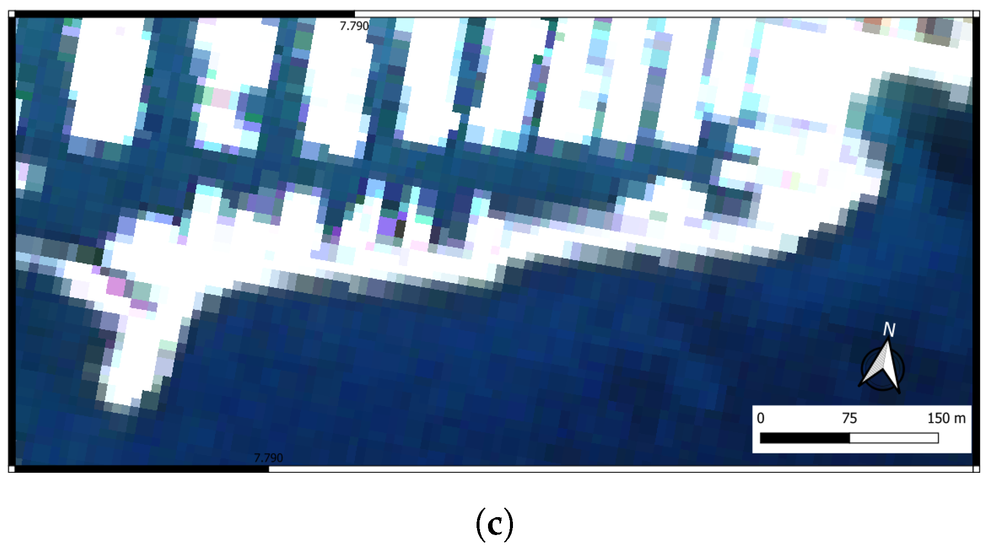
2.2.3. Sentinel-2 Orthophotos

The availability of Copernicus open data and their integration with other spatial data open new horizons to downstream satellite applications in industry [48] while supporting the European scientific community’s efforts to address the increasingly pressing challenges of environmental and climate sustainability.

Copernicus S-2 images, characterized by a revisit time of five days at middle latitudes and a spatial resolution ranging from 10 m to 60 m, were downloaded at Level_2A for both locations from the Copernicus Open Access Hub2 of the European Space Agency (ESA): on April 2019 for Capo San Donato (Table 1) and February 2019 for Portosole (Table 2). Level_2A products [49] were processed upstream with radiometric, 1 m geometric and atmospheric corrections for Bottom-Of-Atmosphere (BOA) reflectances, distributed relative to the WGS84 global reference system and using the UTM cartographic projection, zone 32N (EPSG code: 32632). The selection of images to download was based on the absence of clouds over the study area and the low presence of sun-glint effects. Three bands with a spatial resolution of 10 m, i.e., bands 2, 3, and 4, were used to derive the bathymetry.

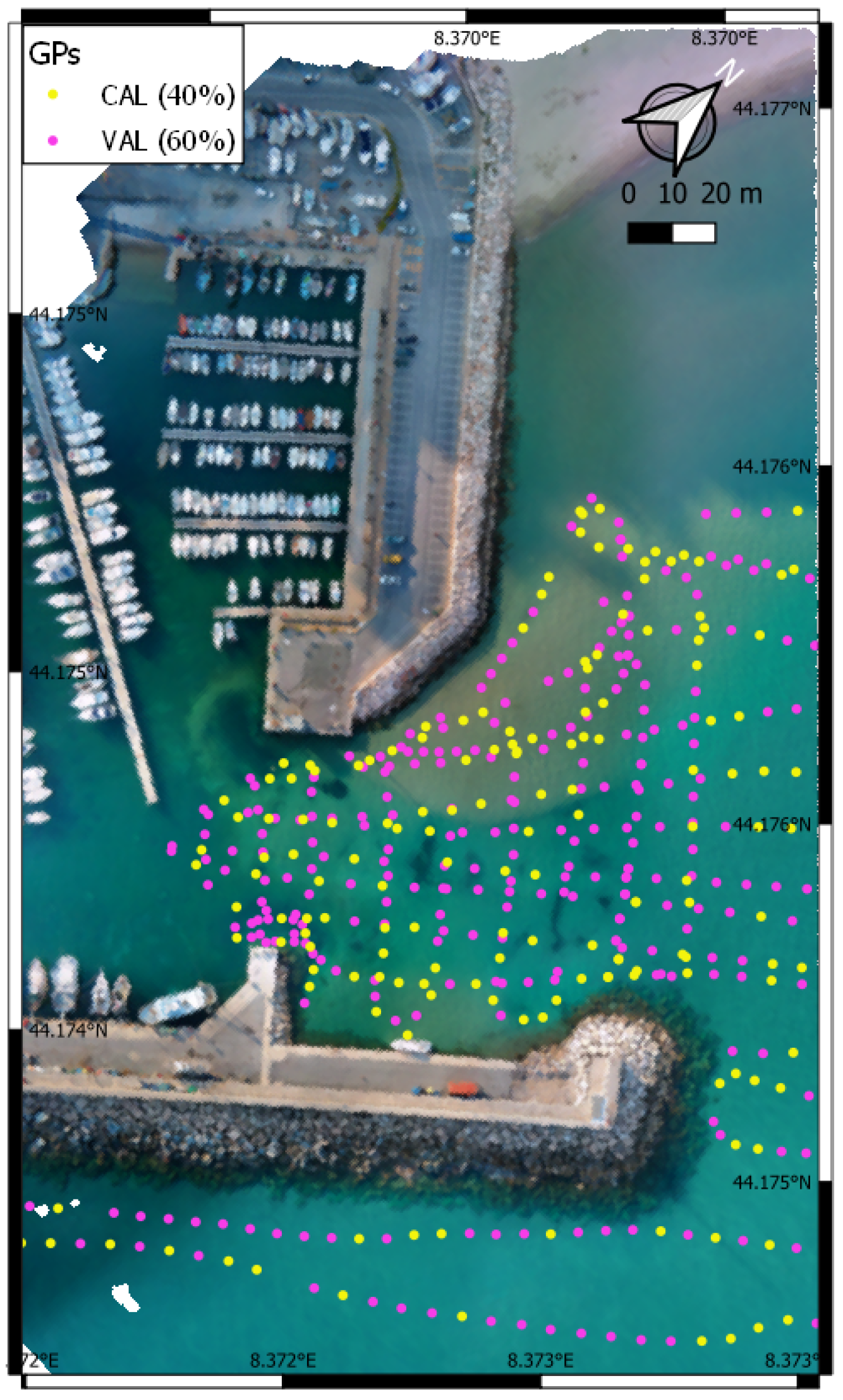
2.3. In Situ Data—Echo Sounding

SBES and MBES surveys related to the AOIs were available and used as reference bathymetry data for the calibration and validation of the RDB method. In fact, they were randomly split into two sets, the 40% used for the calibration of the RDB algorithm and the 60% used for its validation.

Capo San Donato. In situ SBES data were acquired via a Garmin GPSmap 188 Sounder, operating with a dual frequency transducer (50/200 kHz) and equipped with a Leica GS10 GPS antenna, framed in Rome40 datum, with Gauss–Boaga carthographic projection (EPSG code: 3003. The survey was performed on April 2019 by the Maifredi Geological Associated Studio as part of the dredging activities of the access channel to the port of Finale Ligure, commissioned by Finale Ambiente S.p.A. and the Municipality of Finale Ligure. Twenty-six transects oriented according to the axis of the port access channel and eleven perpendicular to them outside and inside the port were surveyed. The total route was about 7600 m for a total of over 1400 points. The bathymetry was derived down to a depth of about 6.5 m. The average point spacing is 10 m.

Portosole. The site was surveyed on February 2019 by Drafinsub Srl. exploiting both MBES and UAV-derived photogrammetry techniques. The Teledyne Reson PDS2000 platform [50] was employed to acquire the bathymetry of the whole area, framed in the ETRS89 reference system, projected in the Universal Transverse Mercator (UTM) zone 32N (EPSG code: 32632). A total of 16,736,828 points constitute the digital model of the seabed with a cell resolution of 10 × 10 cm. The bathymetry was derived down to a depth of 12 m. Further details on the UAV and MBES survey, the processing and the data quality checks, mainly referring to point cloud density and noise, can be found in [3,51].

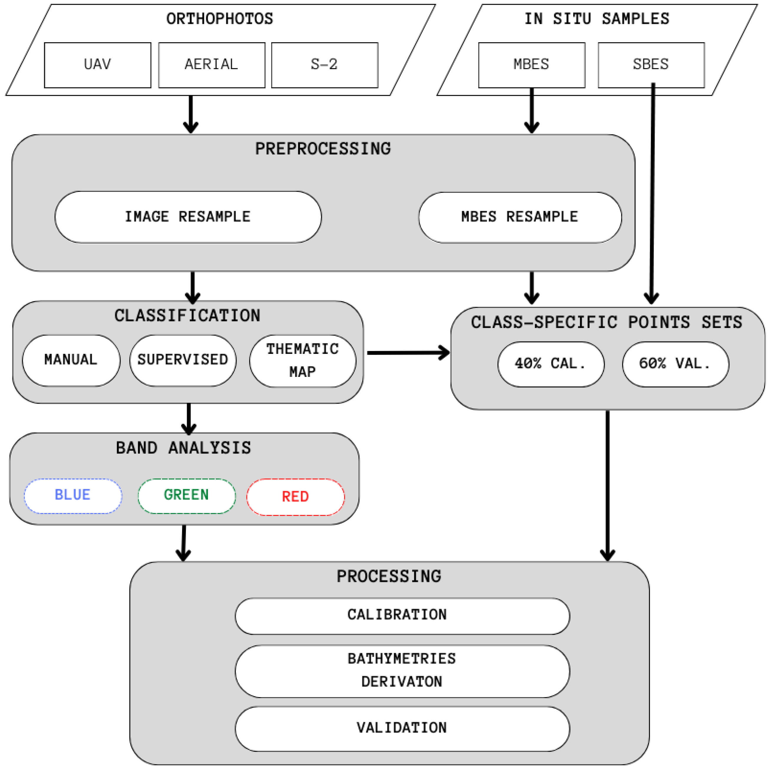
2.4. Remote-Derived Bathymetry Workflow

A bathymetric reconstruction procedure was defined, the core of which is the Stumpf method [28], based on the relationship between pixel radiometric values and known depths.

After the datasets were selected and downloaded, the procedure’s workflow involves (i) the proper pre-processing of orthophotos and ground truth points, aiming at the removal of outliers and/or the filtering of impurities due to reflections on the surface or seabed; (ii) the classification of the seabed into homogeneous classes; (iii) the analysis, selection and combination of bands; (iv) the calibration of the model based on the ground truth data and the bathymetry assessment; and finally, (v) its validation, as represented in more detail in Figure 5.

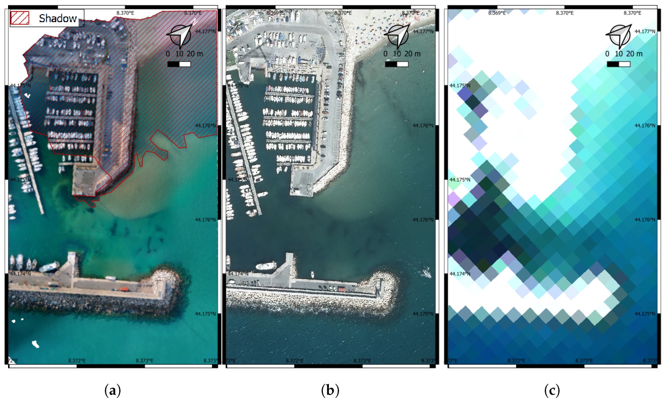
2.4.1. Pre-Processing

The S-2 data were pre-processed in the following steps: (i) sub-setting, to crop the 100 × 100 km² satellite image to the desired AOI; (ii) re-sampling, to geometrically correct multi-size bands to a single-size band image; and (iii) re-projection, to create an image in the proper Coordinate Reference System. Pre-processing of the S-2 data was performed with the Sentinel Application Platform (SNAP) [52] open-source toolbox, made available by the ESA.

Aircraft and UAV orthophotos were re-projected, merged and/or cropped for the AOI selection. The pre-processing was carried out using the free and open-source Geographic Information System QGIS [53]. The free and open-source Geographic Resources Analysis Support System GIS (GRASS) [54] was used for the supervised classification.

Furthermore, it is useful to apply a land mask in order to focus the subsequent procedure on the seaside only. It was applied in QGIS using the most recent (2016) coast vector line available on the Regione Liguria geoportal3.

The in situ MBES sample, usually characterized by high spatial density, could be re-sampled to associate a single depth value to each pixel of the image, thus avoiding having different depths associated with the same color combination.

In this perspective, in the Portosole AOI, MBES was re-sampled at 0.2 m and 10 m spatial resolutions in QGIS, so as to be comparable with aircraft and S-2 images, respectively (see Table 2).

The same procedure is not suggested for the SBES samples because they are less dense and not regularly distributed.

2.4.2. Seabed Classification and Cleaning

The empirical band ratio method proposed by Stumpf [28], based on the relationship between pixel radiometric values and known depths, is affected by the color and type of the seabed. Therefore, when the seabed is characterized by heterogeneous areas, i.e., sand, rock and algae or seagrass, it is suggested to classify the bottom in order to apply Stumpf’s method individually to each seabed class.

While the seafloor of Capo San Donato was essentially uniform and composed of sand, classification was necessary for Portosole, whose seafloor included four categories: sand, natural rock, artificial rock and Posidonia Oceanica meadows.

A pixel-based supervised classification was applied to the aircraft orthophoto of Portosole. It was performed thanks to the maximum-likelihood discriminant analysis classifier i.maxlik4 [55] implemented in GRASS GIS. Classification is based on the spectral signature information generated by i.gensig5 relative to a set of training areas that have to be defined for each class. The training map of the Portosole aircraft orthophoto was defined for four bottom cover classes: sand, natural rock, artificial rock and Posidonia Oceanica meadows. In addition, with the same approach, a further class, “boat”, was identified to remove the outliers given by the presence of boats. Moreover, given the presence of other disturbances in the aircraft orthophoto (i.e., bathers and surface reflections), a low-pass filter was applied to the classified map. In particular, a neighborhood filter of 5 pixels, corresponding to 1 m, was used to re-sample each previously defined class individually. Filtering, which could be applied at the pre-processing stage, is instead suggested after the automatic classification of the seabed so that it does not influence the classification but improves its final result.

In the case of very high-resolution images, such as the UAV-derived orthophoto, the color of the seabed can be “disturbed” by sea-surface reflections and shadows or a single pebble could be identified. It is therefore suggested to proceed with manual digitalization of the different classes by exploiting the visual recognition of seabed classes. In fact, an automatic classifier would require a major a posteriori filtering process or the use of a contextual classification algorithm, which, however, does not always correctly define class boundaries.

In the case of low-resolution images, where no object is clearly identifiable and the contours of a homogeneous area are difficult to define, automatic or manual classification is more complex; hence, the use of a land-cover map, if available, is suggested. The S-2 orthophoto was classified using the thematic map of the New Atlas Of Marine Habitats6, available on the Regione Liguria geoportal. It provides a naturalistic knowledge base of the coastal seabed relative to 2020 at a scale of 1:10,000.

After classification and cleaning, the images and the GPs datasets were masked according to each class’s coverage of the respective orthophoto, including only sandy and (natural and artificial) rocky areas. The Posidonia Oceanica seagrass areas were excluded from the calculation of RDBs due to the high uncertainty in the relationship between the color of the seabed and the depth. In fact, Posidonia is characterized by ribbon-like leaves, about 1 cm wide and up to 1.5 m long, generally moved by sea currents, so the depth in the meadow areas is not easily detectable.

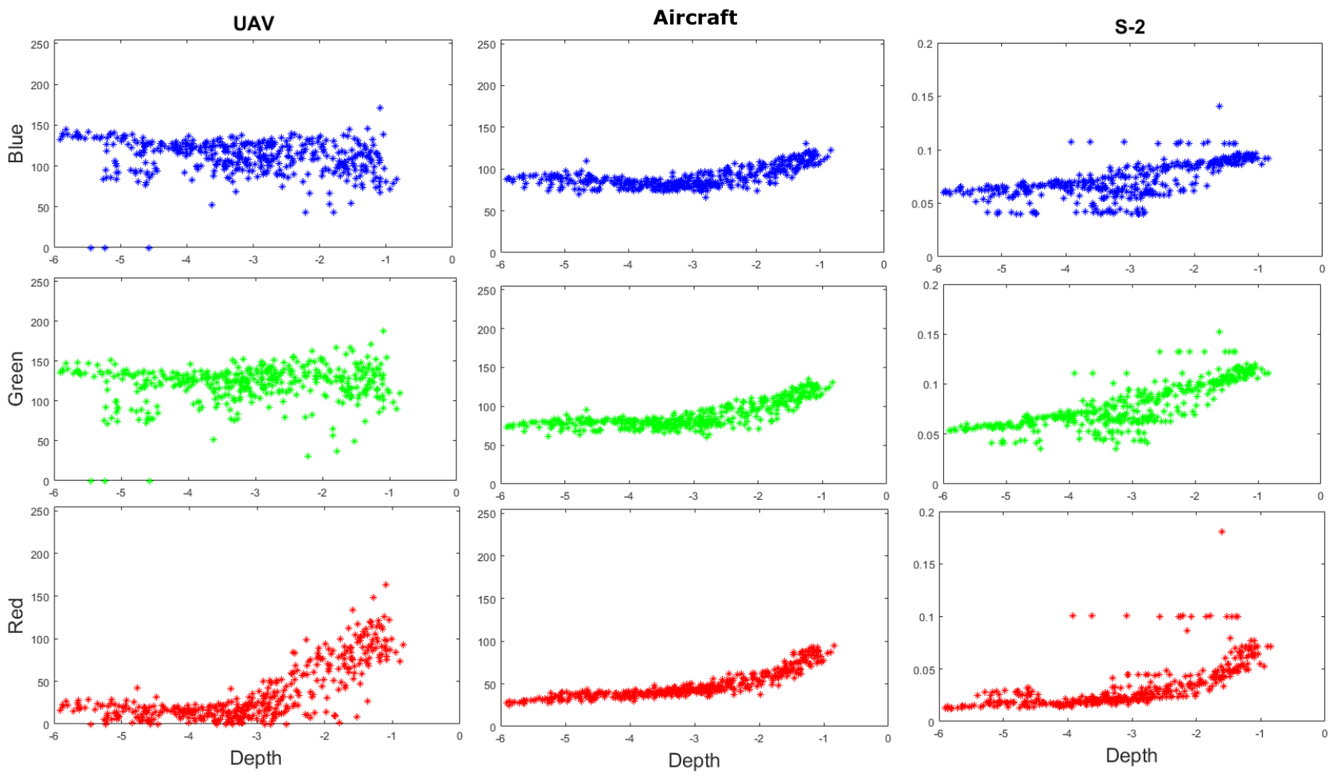
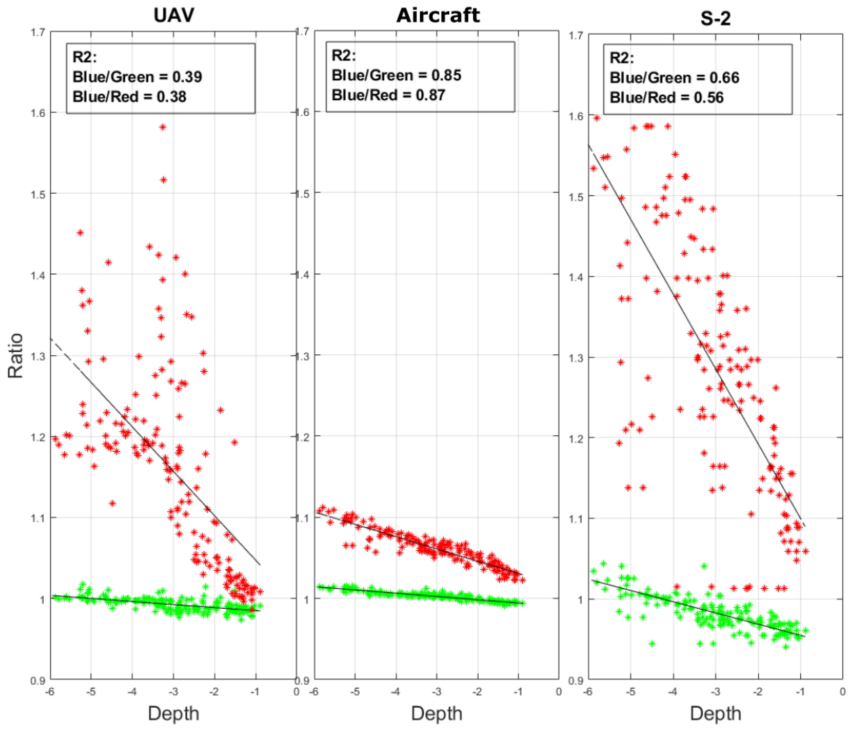
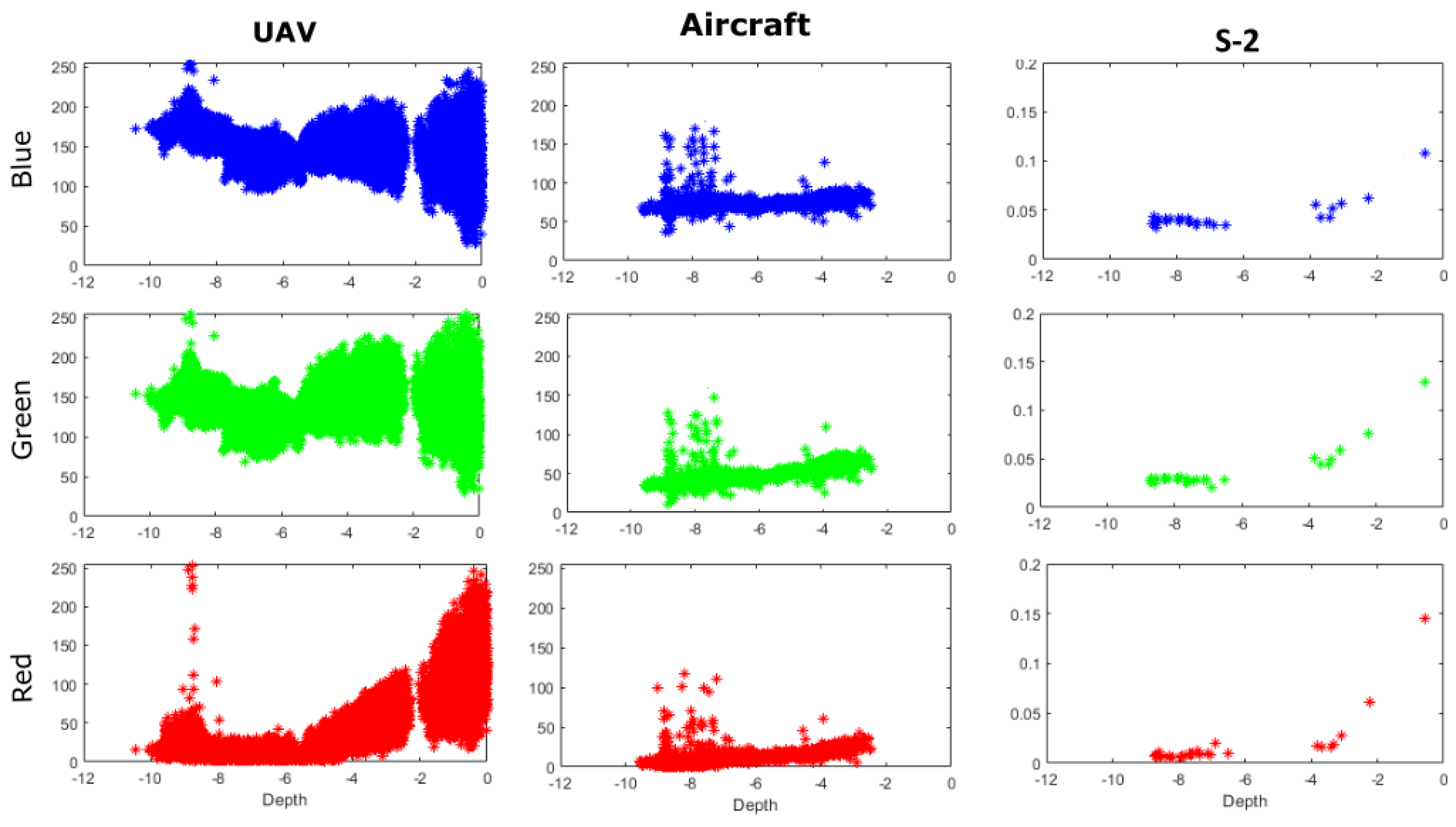
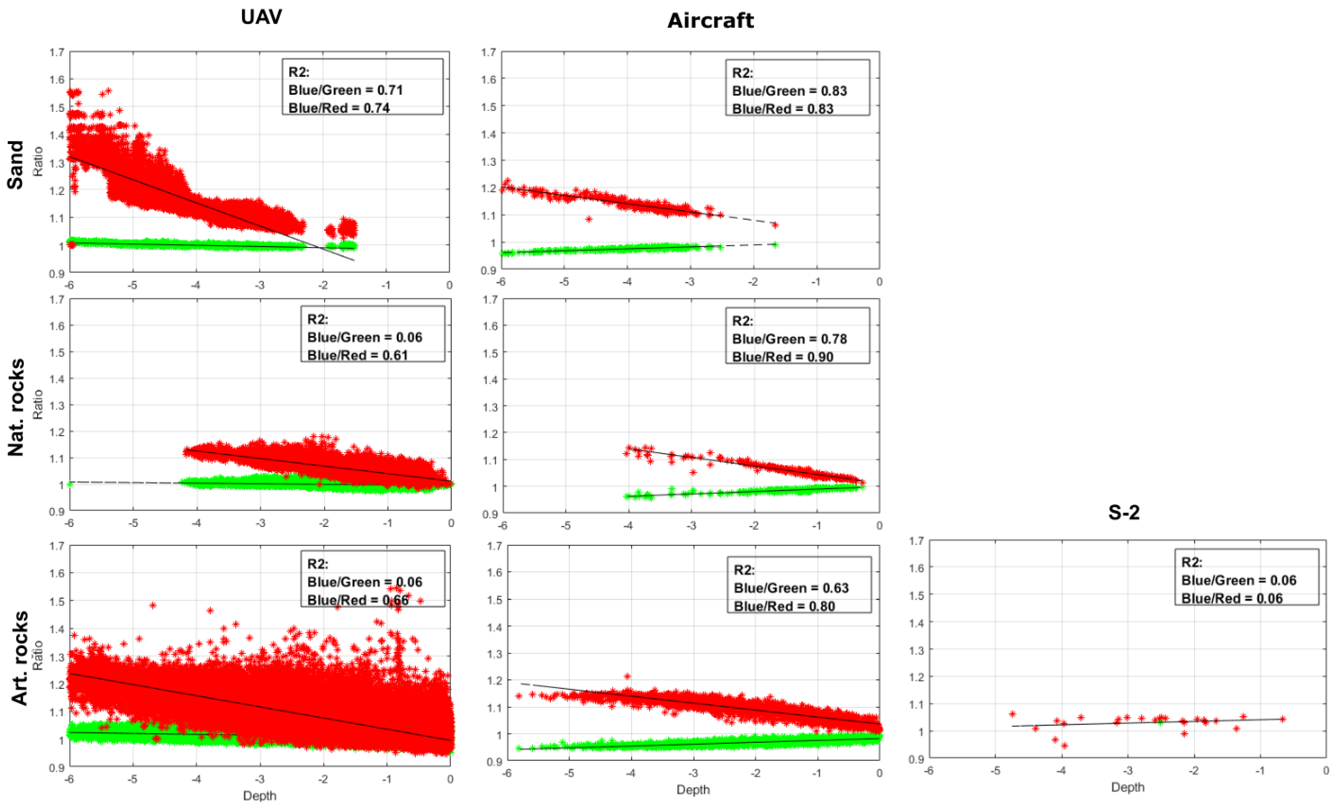
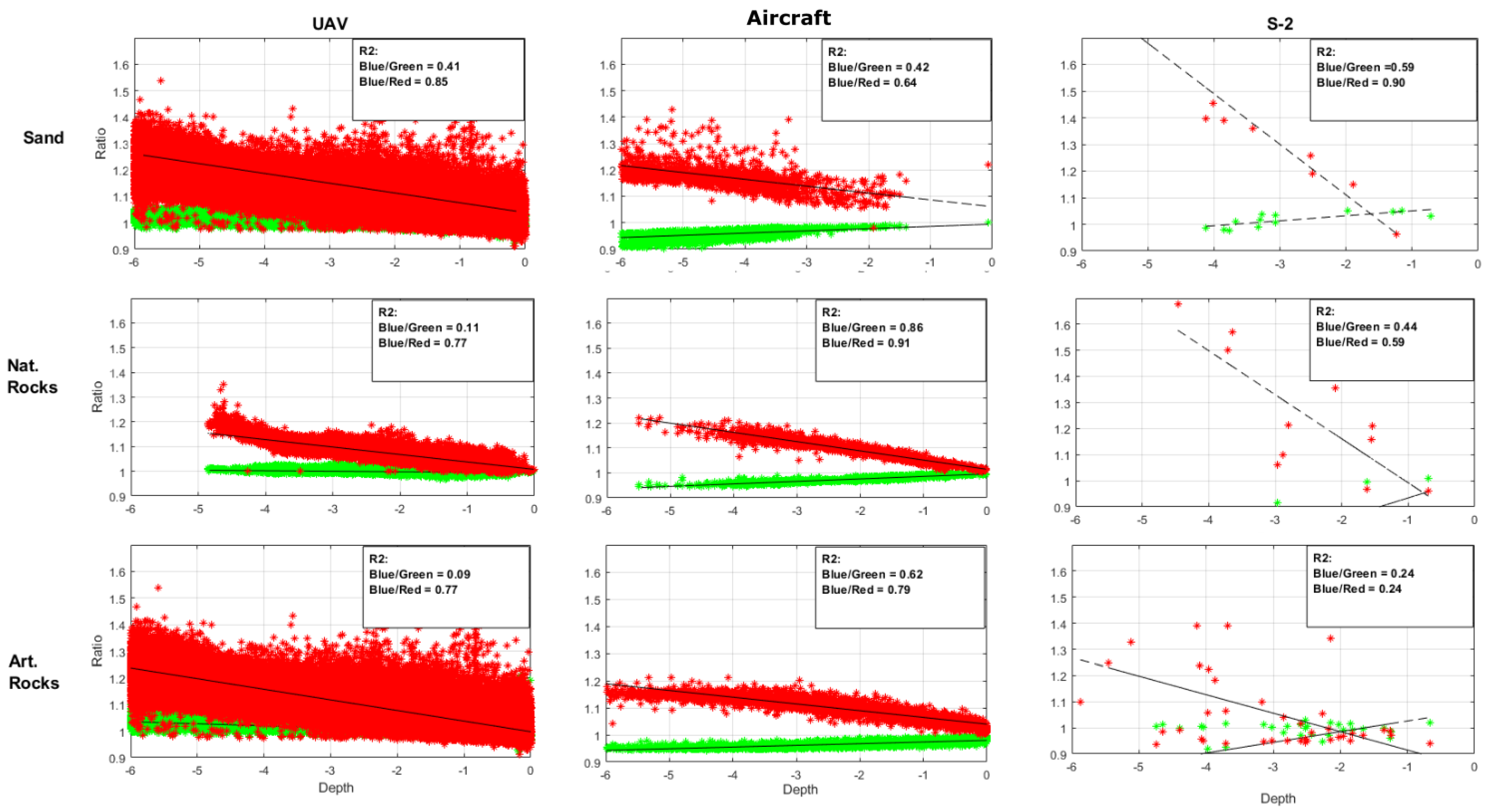
2.4.3. Band Analysis

Stumpf’s method is based on the ability of the different RGB bands to reach the seabed and be reflected by it. Therefore, an analysis of the correlation of the different RGB bands composing the orthophotos with the bathymetric data could be useful both to highlight which bands are most correlated and how this correlation varies with depth. Furthermore, such an analysis could highlight the presence of noise in the response because the same color intensity is associated with different depths.

2.4.4. Processing

Stumpf’s method [28] is described in Equation (1), where Z is the derived bathymetry and m₀ and m₁ are the coefficients to be applied to the bands’ ratios [28]:

$$Z=m_1\frac{ln\left(n{R}_w\left({\lambda }_i\right)\right)}{ln\left(n{R}_w\left({\lambda }_j\right)\right)}-m_0$$

(1)

To apply the method, it is necessary to identify the most suitable bands and to estimate the coefficients m₀ and m₁ [6,28,33,36]. As far as the choice of bands is concerned, Stumpf suggests using the blue band as a reference as the numerator of the ratio and the green or red band as the denominator [56]), depending on the response of the individual bands to changes in the seabed type and depth reached.

The UAV-derived and aircraft orthophotos were resampled to a coarser resolution of 0.1 and 1 m, respectively, to make their high resolutions (as shown in Table 1 and Table 2) more similar to the ones of the ground truth data.

The estimation of the coefficients is conducted through a calibration procedure, which requires having known bathymetry values (GPs) and performing a linear regression between these values and the ratio of the chosen bands. The available GPs were randomly split into two groups: a calibration set of 40% and a validation set of 60% for statistical analysis of the results.

It is suggested to estimate the best values of the coefficients for each AOI, for each platform-derived orthophoto and for each homogeneous seabed type.

Hence, Stumpf’s method is applied so to derive bathymetries for the AOI, which are then validated through statistical analysis.

The validation procedure consists of correlating the estimated depths with the GPs and calculating statistical parameters such as the coefficient of determination R², the Root-Mean-Square Error (RMSE), the Mean Absolute Error (MAE) and the deviation (BIAS). R² is used to identify the strength of the model resulting from data regression. The RMSE measures the differences between values estimated by the model and the observed values, while the MAE measures the average magnitude of the errors in a set of predicted values, without considering their direction [57]. The RMSE and the MAE are used to evaluate the regression model because they demonstrate accurate the prediction is and the amount of deviation from the observed values. The RMSE will always be larger or equal to the MAE; the greater the difference between them, the greater the variance in the individual errors in the sample. If the RMSE equals the MAE, then all the errors are of the same magnitude. Lower values are better for both parameters. For an ideal model, RMSE/MAE = 0 and R² score = 1. The BIAS value, calculated as the “measured value - derived value” (i.e., $GP-Z$) bathymetry value, has positive values when the model overestimates the water depth (higher depth values in absolute terms) and negative values when the model underestimates the water depth. Thus, in the case of overestimated bathymetry, the model gives a result against navigational safety, and vice versa. The deviation average value (BIAS AVG) between the derived bathymetry and the GPs of the validation set and its standard deviation (BIAS STD) measure the goodness of the derived bathymetry and its dispersion, respectively. Note that the BIAS STD is always smaller than the RMSE by definition and is very close to it if the BIAS AVG is close to zero.

3. Results

In Capo San Donato, the extent of the analyzed area corresponds to the dimensions of the UAV image. Thus, both aircraft and S-2 orthophotos were cropped to such an extent. Moreover, due to the shadow of the hill behind the marina (see Figure 3a), some of the SBES points have been discarded, totaling a final GP set of 440 points, 167 points for calibration and 273 points for validation, as shown in Figure 6.

In Portosole, two different area extensions were used: firstly, the areas classified with the same coverage on the different orthophotos, called “overlap” areas, were used to perform a comparison for homogeneous classes; secondly, the analysis was extended to the whole dimensions of the respective orthophotos, called “extended” areas, using specific seabed classification. The latter MBES GPs, resampled at 1 m and 10 m grids for the RDB from aircraft and S-2 orthophotos, respectively, are shown in Figure 7. The RDB derived from UAV orthophotoes used all the available MBES points, which are not represented in Figure 7 because they are too dense.

3.1. Capo San Donato

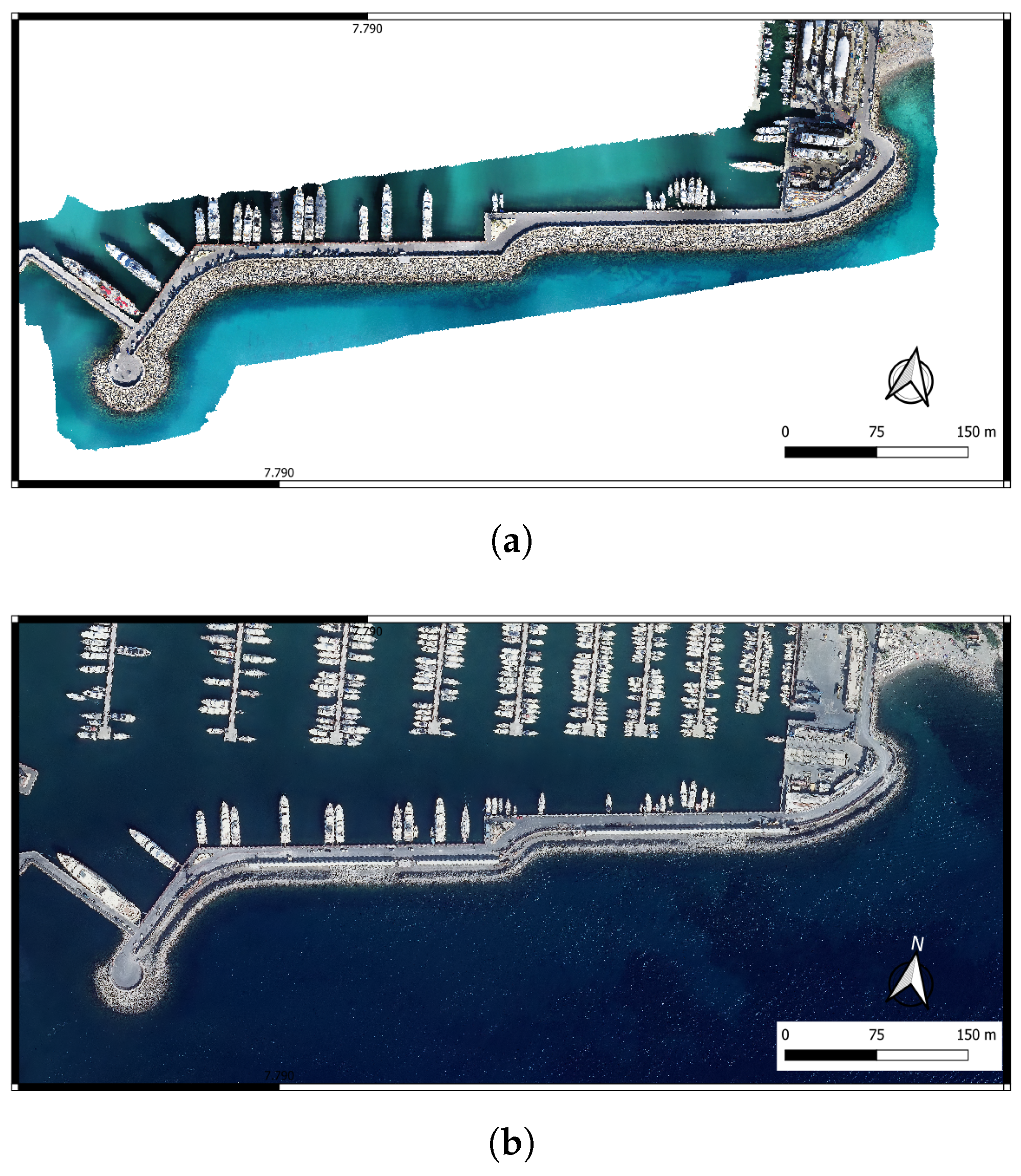
Capo San Donato is a marina characterized by a flat morphology and sandy seafloor. No classification was therefore necessary.

During the workflow’s pre-processing steps, the selected UAV orthophoto required the application of a further mask to remove some sea areas with darker colors from consideration due to the hill’s shadow effect, as depicted in Figure 3a.

A preliminary analysis of the relationship between the RGB bands and depth (m) was performed by sampling individual bands and measuring their respective response to depth. Figure 8 shows the RGB/depth plots for the three orthophotos. A strong variability in the first few meters of depth for all bands, most pronounced in the image acquired by the UAV, is evident. In addition, the red band tends to zero for greater depths, as this band can only penetrate the first few meters of water (refs. [58,59]). The response of the aircraft image is less dispersed than the UAV- and S-2-derived images. Since no band seems to be more correlated with depth than the the others, both blue/green and blue/red ratios were analyzed in the processing phase.

A regression analysis was performed to calibrate the linear model, which measures the relationship between the band ratio and the GPs, as shown in Figure 9. Significant dispersion for depths greater than 2.5 m is evident for both the UAV and S-2 orthophotos, mainly for the blue/red ratio. Instead, the corresponding relationship between the blue/green ratio and the depth seems more defined. In the case of the aircraft orthophoto, the regression using both ratios is characterized by lower dispersion in all the depth classes. This qualitative analysis is confirmed by the values of R², reported in Figure 9.

The R² is quite low for the UAV image (around 0.4) and very high (around 0.85) for the aircraft image; therefore, the linear model defined for the aircraft image correctly reproduces the color–depth correlation, while for the UAV image, this correlation seems very weak. The R² results obtained for the S-2 orthophoto are in the middle. The difference between the results obtained with the two different ratios is more pronounced in the case of the S-2 image, where the blue/green ratio gives better results.

After the calibration, Stumpf’s method was applied to derive the bathymetry for the AOI. Then, the results were validated through statistical analysis, thanks to the RMSE and MAE parameters, as reported in

Table 3. Statistical parameters (in m): RMSE and MAE for the model validation and the average value and the standard deviation of the BIAS between the RDB and the GPs for the two band ratios and the three platforms in sandy areas in Capo San Donato.

		BLUE/GREEN	BLUE/RED
UAV	RMSE	1.53	1.88
	MAE	1.13	1.40
	BIAS AVG	−0.16	0.48
	BIAS STD	1.52	1.87
Aircraft	RMSE	0.71	0.52
	MAE	0.60	0.39
	BIAS AVG	−0.44	−0.08
	BIAS STD	0.56	0.51
S-2	RMSE	0.95	1.05
	MAE	0.71	0.78
	BIAS AVG	−0.38	−0.12
	BIAS STD	0.87	1.04

. The values of the RMSE and MAE confirm that the model employing the green band is slightly better than the one with the red band for the S-2 and UAV orthophotos. The difference, albeit minimal, in terms of accuracy lies in the order of tens of cm. Among the three different orthophotos, the UAV one resulted in higher RMSE, while the aircraft and S-2 orthophotos allowed for more accurate results.

Finally, the average value and the standard deviation of the deviation (BIAS AVG and BIAS STD, respectively) between the derived bathymetry and the points of the validation set were calculated and reported for each study combination in Table 3. Note that a band ratio characterized by lower RMSE results in a negative value of BIAS AVG that is close to zero; consequently, the BIAS STD value is close to the RMSE. Again, the best BIAS parameters belong to the aircraft orthophoto and the blue/red ratio, with deviations of the order of 50 cm. The best solution for the S-2 orthophoto seems to be the blue/green ratio because it has the lowest RMSE value, but a BIAS AVG of almost 40 cm is present, increasing the uncertainty in the accuracy of the RDB. Meanwhile, the BIAS STD for the UAV orthophoto confirms its bad results, with errors of the order of 1.5 m.

Figure 10 shows the best RDBs maps, derived from the orthophotos of the three different platforms using the best band ratio. The real bathymetry seems to be well represented by the RDB, especially the UAV and the aircraft ones, also reproducing, for instance, the sand bar at the marina entrance. The depth model derived by the aircraft orthophoto is smoother, without artifacts due to sudden changes in color, as happens in the UAV model in the entrance channel.

The depth model derived by the S-2 image is obviously approximated due to the low resolution of the image, but, at the same time, represents macro-depth variations well. Moreover, note some unnatural values above sea level in all the platform-derived bathymetries (depicted in green), mainly close to the dry–wet boundaries along the piers.

Figure 11 shows the spatial distribution of the deviation from the derived bathymetry and the SBES’ depths. Mild errors, around or below one meter, are evenly distributed throughout the AOI for the aircraft and S-2 images, except for a localized area near the pier at the marina entrance that is affected by greater negative errors. This area is also affected by error for UAV orthophoto, which also presents a negative BIAS located in the sandbar area. All three derived bathymetries have an area with shallower depths distributed mainly in front of the beach and in the deposition area on the side of the marina entrance channel. In this area, the BIAS for the aircraft orthophoto ranges from −1 to 1 m (Figure 11b), while for S-2 and UAV-derived orthophotos, the error is higher (Figure 11a,c).

3.2. Portosole

The AOI of Portosole is characterized by different classes of seafloor cover: sand, natural rock, artificial rock and Posidonia Oceanica meadows. As discussed in Section 2.4.2, different seabed classifications methods were used because they were considered most effective depending on the degree of detail represented in the image; in particular, manual digitalization, automatic supervised classification and use of the thematic map of the New Atlas Of Marine Habitats were employed for the UAV-derived orthophoto, the aircraft orthophoto and the S-2 image, respectively.

In Figure 12, an excerpt from the AOI of Portosole, related to the beach area close to the marina, is shown. Figure 12a shows the results of the manual classification for the UAV orthophoto; Figure 12b shows the maximum likelihood supervised classification of the aircraft orthophoto; and Figure 12c shows the classification available on the Liguria Region geoportal, related to the Habitat 2020 Directive, used for the S-2 image. The orange, yellow, green and blue areas represent natural rocks, artificial rocks, sand and Posidonia Oceanica areas, respectively. It should be noted that the three orthophotos classify the same area differently, as in the case of the area at the top of the beach, where the presence of sand and natural rocks alternates differently. The classification of the aircraft images was influenced by the presence of boats, swimmers and reflections of sunlight on the sea surface. Areas affected by these noises were excluded before RDB processing.

Figure 13 highlights an excerpt of the areas where the different classifications identified the same class, taking into account sand and artificial rocks. In the limited AOI, there is no overlapping area for natural rock in all three classifications. Natural rock areas only overlap in the UAV and aircraft images. Nevertheless, only the overlapping area of the two orthophotos for natural rocks is shown in Figure 13.

The RDB workflow will be first applied to these so-called “overlap areas” in order to compare the results from the different types of orthophotos for homogeneous classes. Then, the RDB method was extended to the whole AOI for each orthophoto and for each seabed class, and the derived bathymetry was analyzed.

3.2.1. Portosole Overlap Area

A preliminary analysis of the relationship between each RGB band and the depths of the GPs was performed for each seabed class and each orthophoto in the overlap area. Given the limited extent of the overlap area, the number of points relative to S-2 orthophoto is very low, compared to aircraft and UAV-derived cases, as shown in

Table 4. Number of calibration and validation points used for each type of orthophoto (UAV, aircraft and S-2) for the three considered classes (sand, artificial and natural rocks). Portosole overlap area.

	SAND		NAT. ROCK		ART. ROCK
	Cal.	Val.	Cal.	Val.	Cal.	Val.
UAV	28,964	43,402	24,325	36,077	211,658	317,786
Aircraft	297	430	257	359	2097	3233
S-2	4	5	-	-	25	28

. Remember that the very dense MBES points were resampled at different resolutions, 10 cm, 1 m and 10 m, so as to be closer to the UAV, aircraft and S-2 images’ resolutions, respectively.

In Figure 14, the band/depth correlation trend for the sand class is depicted. The plots for the UAV image have very high dispersion due to the high level of details visible on the seabed causing high variability in colors. Moreover, the aircraft plots highlighted several outliers beyond 7 meters. In all the graphs, the red band signal decreases rapidly to zero in the first 5–6 m of depth because this wavelength is mostly absorbed by the water column at higher depths (refs. [58,59]). Consequently, to reduce the band ratio noise in the following calibration results and in order to be able to test the ratio with the red band too, all the following RDB models were calibrated in the depth range of −6 to 0 m only, for all the classes.

Figure 15 shows the band/depth correlation trend for the aircraft image and all three seabed classes. The artificial rocks are characterized by highly variable colors, especially at shallow depths, probably due to the shadows produced by the large square blocks. Therefore, for this class, the estimation of depth could be more uncertain. On the other hand, in the case of sand, the band/depth correlation is clearly defined, although not very strong; indeed, the slope of the curve is very weak. The area classified as natural rocks has a well-defined band/depth correlation, even if it has some outliers.

A regression analysis was performed to calibrate the linear model relative to each class and orthophoto in the “overlap area”. Each image was masked so as to visualize only the considered class, and the MBES points were divided into a calibration set and validation set for each class. Therefore, the MBES numerosity, shown in Table 4, depends on both the class considered and the geometric resolution of the analyzed image because the points were resampled so that there is one point for every pixel in the image. Note that an insufficient number of GPs characterized the sets relative to S-2 (only 4 for sand, 0 for natural rock and 25 for artificial rock) due to the very low number of pixels describing the different classes in such a small area considering the 10 m resolution of the satellite image. For this reason, the calibration and validation phases will not consider this platform for the overlap areas, postponing the comparison of the S-2 images with those of the other platforms in the next section.

In the calibration phase (Figure 16), higher R² values are detectable for aircraft orthophotos (0.83 for sand and both ratios, 0.90 and 0.8 for the blue/red ratio for natural and artificial rocks, respectively). Both band ratios show a good correlation with depth, even if they have different trends: the blue/red ratio (depicted in red in Figure 16) has an increasing trend with depth (from −6 to 0 m) while the blue/green ratio (depicted in green in Figure 16) decreases with depth.

The blue/red ratio works well for the UAV orthophoto (the R² values are equal to 0.74 for sand and 0.61 and 0.66 for natural and artificial rocks, respectively), even if the correlation has a high dispersion. Instead, looking at the blue/green ratio, the trend is almost horizontal for the UAV orthophoto, i.e., the ratio does not change with depth.

On the contrary, for S-2 the correlation is very low, with a decreasing trend without distinction by band ratio.

Through the calibration phase, the regression parameters were identified for each seabed class and orthophoto and used to apply Stumpf’s method (Equation (1)) to derive the bathymetry in the overlap area. The results were validated through statistical analysis, as reported in

Table 5. RDB statistical parameters (in m) for each platform (UAV, aircraft and S-2): RMSE and MAE for the model validation and AVG and STD BIAS between the RDB and the GPs for the two bands ratios for each seabed class (sand, artificial and natural rocks). Portosole overlap area.

		SAND		NAT. ROCK		ART. ROCK
		BLUE/GREEN	BLUE/RED	BLUE/GREEN	BLUE/RED	BLUE/GREEN	BLUE/RED
UAV	RMSE	0.54	0.51	2.52	0.68	5.01	0.85
	MAE	0.43	0.43	1.75	0.51	3.35	0.65
	BIAS AVG	−0.26	−0.31	1.06	0.36	2.21	−0.19
	BIAS STD	0.47	0.41	2.29	0.57	4.49	0.83
Aircraft	RMSE	0.52	0.60	0.44	0.46	1.05	0.92
	MAE	0.45	0.53	0.33	0.41	0.82	0.77
	BIAS AVG	−0.40	−0.51	0.23	0.38	−0.49	−0.71
	BIAS STD	0.33	0.31	0.38	0.25	0.93	0.58
S-2	RMSE	-	-	-	-	3.52	3.44
	MAE	-	-	-	-	2.80	2.49
	BIAS AVG	-	-	-	-	−0.72	0.30
	BIAS STD	-	-	-	-	3.51	3.49

. The blue/red ratio outperforms the blue/green one five times out of seven. In particular, it is always better for artificial rock and all three platforms. The best RMSE values for the other two seabed classes and platforms alternate, although they remain very close to each other, except for the natural rock for the UAV image, which shows very high values using the blue/green ratio.

Bathymetry in the sandy seabed can be derived with an RMSE around 0.5 m for the UAV and aircraft orthophotos. Instead, in natural rock areas, the bathymetry can be derived with 0.44 and 0.68 m RMSEs for the aircraft and UAV orthophotos, respectively. The complexity of the artificial rock seabed leads to higher RMSEs, around 0.9 m for UAV and aircraft images and more than 3 m for S-2.

Finally, the average value and the standard deviation of the deviation (BIAS AVG and BIAS STD, respectively) between the derived bathymetry and the points of the validation set were calculated and reported for each combination in Table 5. Note that no BIAS AVG is close to zero, as happened for the best band ratio in Capo San Donato AOI. Most of the BIAS AVG values are negative, with absolute values ranging between 0.19 and 0.71 m. BIAS STD is close to the RMSE or lower, as expected.

In conclusion, UAV and aircraft images allowed us to derive bathymetry with the same accuracy, which is comparable for sand and natural rocks and lower for artificial rocks, in the overlap area. S-2 images were tested but did not yield good results because of the low number of pixels in the analyzed area led to a weak regression.

3.2.2. Portosole Extended Area

To make a more exhaustive comparison between the three platforms, considering the data of S-2 for all three seabed classes, the original extent of each orthophoto and its specific classification were taken into account. In this way, the number of GPs for each orthophoto was significantly increased compared to those of the overlap area, as shown in

Table 6. Number of points used for each type of orthophoto (UAV, aircraft and S-2) in the two different sets (calibration and validation) for the three considered classes (sand, artificial and natural rocks). Portosole extended area.

	SAND		NAT. ROCK		ART. ROCK
	Cal.	Val.	Cal.	Val.	Cal.	Val.
UAV	40,252	60,754	47,059	68,253	427,636	642,000
Aircraft	1683	2474	1741	2555	3496	5311
S-2	13	17	11	24	41	63

. Concerning the S-2 image, it should be noted that the number of available GPs for both calibration and validation is always low, in the order of tens for all classes, due to the high pixel size compared to aircraft and UAV images.

Figure 17 shows the relationship between the depth and the blue/green ratio (depicted in green) and the blue/red one (depicted in red) for all the platforms and all the seabed classes. It highlights the same trends and characteristics already described for the overlap area (Figure 16), as follows.

Even if the UAV plots are characterized by a high dispersion, the R² is high, ranging from 0.77 for natural and artificial rocks to 0.85 for sand using the blue/red ratio, whereas the correlation for the blue/green ratio is considerably lower and negligible for natural and artificial rocks.

Also for the aircraft image, the blue/red ratio gives better results, with an R² ranging from 0.64 for sand to 0.91 for natural rocks. As for the overlap area, the blue/green ratio decreases with increasing depth. The S-2 image allows us to define a good correlation for sand, especially for the blue/red ratio (R² = 0.9), while the correlation for natural rocks is weaker (R² = 0.59 for the blue/red ratio). The artificial rocks are very difficult to model with S-2 because they are distributed along a thin layer close to the breakwater and hence are not clearly characterized inside the 10 m × 10 m pixels.

Table 7. Statistical parameters (in m) of the RDB with the three different platforms (UAV, aircraft and S-2) for the three considered classes (sand, artificial and natural rocks). Portosole extended area.

		SAND		NAT. ROCK		ART. ROCK
		BLUE/GREEN	BLUE/RED	BLUE/GREEN	BLUE/RED	BLUE/GREEN	BLUE/RED
UAV	RMSE	1.94	0.96	2.85	0.60	5.37	0.91
	MAE	1.62	0.73	2.17	0.44	4.04	0.68
	BIAS AVG.	0.32	0.69	−0.02	0.24	−0.37	−0.07
	BIAS STD	1.95	0.66	2.82	0.54	5.35	0.90
Aircraft	RMSE	1.11	0.7	0.61	0.51	1.15	0.92
	MAE	0.94	0.57	0.49	0.41	0.92	0.73
	BIAS AVG.	0.16	−0.05	0.38	0.37	0.18	0.56
	BIAS STD	1.09	0.70	0.46	0.36	1.13	0.73
S-2	RMSE	1.0	0.74	1.03	1.28	1.98	1.95
	MAE	0.89	0.60	0.90	1.11	1.44	1.45
	BIAS AVG.	0.72	0.57	−0.14	−1.12	1.98	0.19
	BIAS STD	0.88	0.47	1.03	0.62	1.96	1.95

shows statistics to validate the results for the extended area. The blue/red ratio outperforms the blue/green ratio eight times out of nine. Especially in the case of the UAV image, the blue/red ratio allows for greatly improved results. Table 7 also reports the BIAS STD values, which confirm the better performance of the blue/red ratio compared to the blue/green one in all cases.

In sandy areas, the RMSE values for the S-2 orthophoto (0.74 m) are very close to those for the aircraft image (0.7 m), while the RDB from the UAV image is characterized by higher RMSE (0.96 m), probably due to the high details of the UAV image that allow us to also see shadows on the seabed cause by ripples.

For areas classified as rock, both natural and artificial, the RMSE values for the S-2 orthophoto (1.03 and 1.95 m, respectively) are almost twice as high as those for aircraft (0.51 and 0.92 m, respectively) and UAV (0.60 and 0.91 m, respectively) orthophotos.

Figure 18 shows the bathymetry derived for all the different images by merging the results obtained for each seabed class using the best band ratio. The differences in spatial resolution in the derived bathymetry values, very high for UAV and too low for S-2, especially near the breakwater, seem to suggest again that the aircraft orthophoto is the best-fitting solution because it is smooth and, at the same time, it is able to accurately reproduce the pattern of the seabed. However, unnatural discontinuities in bathymetry are evident at the boundaries between the different seabed classes. Moreover, note some unnatural values above the sea level both in the UAV and in the aircraft RDBs, close to the dry–wet boundary mainly along the breakwater (depicted in green).

Figure 19 shows the spatial distribution of the deviation from the derived bathymetry and the MBES depth (i.e., the BIAS) for the three platforms.

The UAV RDB seems to slightly overestimate the depth of sand and natural rocks, while it slightly underestimates the depth of artificial rocks. Note that the classes are distributed as shown in Figure 12. This pattern is confirmed in Table 7, where the BIAS AVG values for sand and natural rock are positive while the value for artificial rock is slightly negative.

Instead, the aircraft RDB seems to underestimate the depth in the sand area (distributed as shown in Figure 12) and overestimate the depth in the natural and artificial rocks. This pattern is confirmed in Table 7, where the BIAS AVG value for sand is slightly negative while the value for natural and artificial rock is positive.

Finally, the S-2 RDB is not easily interpretable, as it shows little information due to the low resolution of the S-2 image. In the S-2 RDB, the errors are evenly distributed throughout the AOI and there are no artifacts or areas affected by the major errors.

4. Discussion

The obtained RDB results are analyzed in detail in Section 4.1; some considerations on the methodological approach related to seabed classification follow (Section 4.2); and finally, a comparison of the three platforms in relation to the produced RDBs (Section 4.3) conclude the section.

4.1. Results Analysis

The obtained results show that the aircraft-derived bathymetry is generally more accurate than the UAV and S-2 RDBs in all the analyzed scenarios due to the smooth color of the aircraft orthophoto and its ability to reproduce a model of the seafloor with a considerable level of detail. This is reflected in the statistical parameters reported in Table 3 and Table 7, by looking at the RDB maps (Figure 10 and Figure 18) and at the spatial distribution of BIAS values (Figure 11 and Figure 19), but also analyzing some transects, such as the ones depicted in Figure 20 and Figure 21, showing the RDB profiles for the three platforms and the corresponding GPs along a transect in Capo San Donato and in Portosole, respectively. In Figure 21, the seabed classification along the transect for each platform is indicated, too.

The comparison of the S-2 RDB with the aircraft one shows that the worse values of the former are mainly due to the low resolution of the S-2 orthophoto, which returns only an approximate representation of the surface. Figure 22 shows the differences between the MBES interpolation and RDBs for the Portosole beach area excerpt, considering classes’ distribution shown in Figure 12, with ad hoc seabed classification for each kind of orthophoto, as explained in Section 3.2.2. The areas affected by the greatest error are those at the border between sand and artificial rocks, both for the UAV image and for S-2, where the RDBs tend to overestimate the depth.

For Capo San Donato, Figure 20 shows that at distances between 40 m and 60 m along the transect, the values of two/three pixels of S-2 RDB differ greatly from the MBES data. A similar decay in the accuracy of S-2 RDB is seen in the extended area of Portosole (Figure 21). Approaching the pier, moving from sand to artificial rocks (from the 60-meter transect onward), the deviation of the S-2 RDB from the MBES is in the order of meters.

As for the UAV RDB, the worst RMSE values compared to aircraft ones are for Capo San Donato (RMSE 1.53 m vs. 0.52 m). Figure 20 shows how the UAV RDB profile (in blue) is extremely noisy/variable, greatly diverging from the few SBES points (in red), especially in the first 40 meters of the profile, in contrast with the aircraft RDB line. In the first 20 meters, the UAV RDB also has unnatural values above the sea level (as also shown in green in Figure 10). As can be seen from the orthophoto on the right of Figure 20, these first 40 meters of the transect pass through a sand bar (outlined by a yellow dashed line) characterized by a visibly different color from the surrounding sand. This dissimilarity is also a possible cause of the color band noise (Figure 8) of the UAV signal recorded around −1 m and −2 m elevations. In addition, the UAV RMSE values in the case of San Donato are about 50% higher than those calculated in Portosole, maybe due to the different quality of the two UAV orthophotos, as can be appreciated in the two zoom-ins on a sandy area of the two AOIs in Figure 23a,b.

The present analysis also revealed the impact of band choice on RDB results. It should be remembered that the red band signal decreases rapidly to zero in the first 5–6 m of depth, as this wavelength is mostly absorbed by the water column for higher depth [58,59]. Consequently, to compare the ratios with the green and red bands, and because the San Donato AOI depth is limited to 6 m, the RDB method was applied in the depth range from −6 m to 0 m only. In most cases, the blue/red ratio outperforms the blue/green ratio, as confirmed by the values in Table 7 and by Figure 17, in which the regression with the blue/green ratio is less steep than the one using the blue/red ratio. Capo San Donato shows a partial exception: the blue/green ratio gives slightly better results for UAV and S-2 platforms (Table 3). Looking at Figure 9, the regression graphs for the blue/red ratio and the UAV or S-2 platforms are steeper but also noisier than the one using the blue/red ratio.

Wanting to assess the greater or lesser ability to estimate bathymetry with different seabed classes, note that natural rock tends to return lower RMSE values than the other two classes. In the second zoom-in in Figure 23b, the artificial rocks, which constitute the breakwater, are noticeably angular/square, causing a non-uniform color at a given depth, which produces a higher RMSE.

By comparing the values in Table 7 with those in Table 5 relating to Portosole over the overlapping and the extended areas, respectively, it can be seen that the RDB results can vary significantly. Indeed, the RMSE values in the extended area increase compared to those found in the overlap area in all platform/seabed combinations, except for the natural rocks in the UAV orthophoto and the artificial rocks in both the S-2 and aircraft orthophotos. This can be explained by the higher number of points used for the calibration and validation of the model for the extended area with respect to the overlap area. Moreover, as previously noted, the three orthophotos classify the same areas differently (see Figure 12 and Figure 13), as in the case of the top of the beach area, where the presence of sand and natural rocks alternates differently, affecting the statistics.

4.2. Seabed Classification

The methodological approach of the present paper proposes classifying the images before computing the regression between the ground truth bathymetry values and the ratio of the chosen bands, paying particular attention to the influence of image resolution. Indeed, as already stated in Section 2.4.2, given the specific characteristics of the UAV-, aircraft- and S-2-derived orthophotos, they were classified manually, with a pixel-based supervised classification and using an available cover map, respectively. Then, a regression analysis was performed to calibrate the linear model relative to each class and the platform-derived orthophotos.

On the contrary, most of the examined literature does not classify the seabed or provide a simultaneous retrieval of the bathymetry, the seabed classification and, eventually, the water’s optical properties contextually to the regression procedures [29,30,36,44]. To achieve this, the reflectance spectra of the seabed classes have to be parameterized and the water property information should be available. In addition, it is crucial to perform accurate atmospheric correction, making the methodology complex to implement and possibly slower from a computational point of view [12] because of the need to define a class-specific linear regression model for each defined seabed class.

4.3. Platform Comparison

RDB workflow was applied to the UAV, aircraft and S-2 images in the same AOI, with the aim to analyze the usefulness of different types of images, mainly according to their different spatial resolutions.

The results show that the aircraft orthophoto is the best-fitting solution because it is smooth and, at the same time, can truthfully reproduce the pattern of the seabed. A possible limitation of this result, especially concerning its replicability in other contexts/AOIs, is related to data availability: indeed, the employed aircraft orthophoto is only freely distributed through the WMS service and released with prior authorization for research purposes. Moreover, currently, this product is available in Italy every three years, due to the high cost of the survey phase, unlike the revisit time of a few days of the S-2 or the possibility of carrying out UAV surveys quickly and at low-cost.

The S-2 orthophotos did not allow us to obtain an accurate bathymetry due to its low spatial resolution. Nonetheless, the seabed trend was reproduced correctly, excluding the portions of the study areas close to the coast, i.e., where the single pixel overlaps even only partially with the mainland, and those characterized by a sudden change in depth, as occurs in Portosole near the breakwater.

The UAV-derived orthophotos have a very high resolution, which generates noise in the derivation of the depth of the seabed, as is evident in Figure 20 and Figure 21. Therefore, the RDB would require the application of a low pass filter, so eliminate the high frequencies, i.e., the short signal wavelengths.

Among the literature reviewed, only Rossi et al. [33] compare results obtained using images acquired by different platforms, i.e., UAV and very high spatial resolution satellite images, validating the results with echo-sounder data. No one has compared UAV, aircraft and S-2 images in the same area, as proposed in the present paper.

Rossi et al. [33] applied both the Stumpf [28] and Lyzenga [27] algorithms to derive the bathymetry of a small area along the Tuscany coast (Italy). Their studied areas are characterized by a sandy seabed, similar to the AOI of Capo San Donato in the present contribution.

The UAV images were acquired at an altitude of 150 m, about four times higher than our UAV flight; therefore, Rossi et al.’s images are not characterized by a very high resolution like our UAV images, where the color of the seabed is “distorted” by the reflection of the sea surface and shadows due to individual pebbles or ripples in the sand. Moreover, the UAV images in Rossi et al. were acquired by a multispectral camera, in the same WorldView-2 satellite sensor spectral bands. This permitted to the authors to test new ratio bands, namely, coastal-blue/green and yellow/green, compared with the more traditional blue/green and green/red combinations. UAV-derived bathymetry (UDB) permitted an accuracy of about 30–40 cm in the range 0–5 m and about 1 m in the range 0–11 m.

Satellite-derived bathymetry (SDB) using WorldView-2 images was tested too. Such a sensor has a higher spatial resolution (panchromatic 50 cm res + 8 multispectral bands at 2 m res) than Sentinel-2 one. The authors highlighted that it was not easy to find high-resolution satellite images with good overcast weather and sea conditions; the satellite image was acquired in December 2016 while the UAV one was acquired in April 2018. Obviously, this fact represent a serious impediment in the case of bathymetric monitoring. A higher deviation of the SDB than the UDB from the real sea bottom was generally visible, and deviations also increase with the depth of the bottom.

Due to the difference in spatial and spectral resolutions of the images used by Rossi et al. [33], a direct comparison with our results is not possible. However Rossi et al. indirectly confirmed our observation relative to the need to use UAV images with lower spatial resolution to obtain colors more correlated with depth, not disturbed by local noise.

5. Conclusions

The present research is focused on the comparison of image-derived bathymetry obtained from three platforms, UAV, aircraft and satellite, and applied to two marina areas of the Mediterranean Sea on the western Ligurian coast (Italy). In particular, the entrance of the small marina of Capo San Donato, characterized by sand and a depth lower than 6 m, and the sand and pebble area in front of the beach adjacent to the Portosole marina and outside its artificial breakwater were analyzed. Both areas are interested in sediment deposition or scouring, which can compromise navigational safety or breakwater stability, respectively.

During the application of the RDB workflow, it was deemed necessary to both classify the seabed and resample the very dense MBES data. Classification is necessary to find the best correlation between color and depth for different types of seabed. Moreover, in order to reduce the noise of this correlation, it is recommended to resample the echo-sounding data, which represent the ground truth during the calibration and validation phases, so that only one depth is associated with each pixel in the image.

The seabed classification was carried out using different procedures for different platforms in order to obtain the best results depending on the degree of detail and resolution of the image. In particular, manual classification was applied to the UAV orthophoto, the maximum likelihood supervised classification to the aircraft orthophoto and the thematic map of the New Atlas Of Marine Habitats to the S-2 image.

The comparison between the RDBs obtained from the orthophotos produced by the different platforms was conducted firstly on the areas of overlap, i.e., where the seabed classes identifiable in all three orthophotos coincided. For Capo San Donato, these coincided with the entire orthophoto (with the exception of a shaded area), while for Portosole, these corresponded to a portion of the original orthophotos, the so-called “overlap area”. In both areas, the RDB method was applied and the critical evaluation of the results was performed. Taking into account that the overlap area of Portosole corresponded to a rather small subset of the MBES GPs compared to those available, in a second step, the application of the RDB method was performed on the entire coverage of each available orthophoto.

The RDB workflow was applied for homogeneous classes of the seabed. For each of the three analyzed seabed classes (sand, natural rocks and artificial rocks) and for each platform, the blue/red and blue/green band ratios were tested to check which one yielded the best statistical parameters. In most cases, the blue/red ratio correlates more strongly with depth than the blue/green ratio in the analyzed −6–0 m range. Then, for each platform and for each class, the best band ratio was identified and the RDB method was applied. Finally, the bathymetries derived for each class were merged to obtain a single bathymetric surface for each platform.

The best RDB results seem to suggest that, among the three platforms, the aircraft orthophoto is the most suitable solution. However, it has a limitation in terms of replicability due to its high cost and the long revisit time of the aerial acquisition. The S-2 orthophoto did not provide accurate bathymetry due to its low spatial resolution, but the seabed trend was correctly reproduced. Furthermore, S-2 images are available as open data with a revisit time of only a few days. Finally, the used UAV-derived orthophotos have too high spatial resolutions, which generates noise in the depth definition process. Flying at a higher altitude could easily solve this problem, allowing for frequent and low-cost image acquisition.

Recurring bathymetric surveys are often necessary to improve the usability of marinas by larger vessels and to monitor erosion near the breakwaters that protect the harbor. Hence, a procedure for a quick, not-so-accurate but inexpensive assessment of the state of the seabed and its evolution could be useful to verify the need for a detailed survey, dredging or nourishment and also to support expeditious REA surveys in coastal shallow marinas. With this in mind, although the results obtained by S-2 are not always superior to those of other platforms, the potential offered by this platform to update the derived bathymetry weekly, at only the cost of processing the orthophoto using the method we have outlined, makes it an efficient and effective solution for observing macro changes in bathymetry. Should the analysis from S-2 show the need for more detailed monitoring, this could be carried out with a high-altitude UAV flight (as carried out by Rossi et al. [33]).

In summary, the key elements of the present study deal with (i) the evaluation of the best image classification method and its impact on the RDB, taking into consideration the image resolution; (ii) the individuation of the most suitable band combination according to the previous seabed classification to obtain a single regression law to be applied on the several seabed classes; and (iii) an analysis of three different orthophoto acquisition platforms to derive RDB values on two AOIs. Moreover, particular attention is given to the coherence between the spatial and temporal contextuality of orthophotos and ground truth data.

Possible future perspectives of this work can conduct in-depth-analysis on the best classification method (preceding/contextual to RDB retrieval) and a comparison of the obtained RDB results with those coming from a contextual RDB and seabed classification in the regression procedure. Indeed, some challenging aspects still remain in both cases, such as the over/under-estimation of depth values due to local reflectances and shadows, e.g., the artificial rocks of the Portosole breakwater causing a non-uniform color at a given depth and a consequently higher RMSE in RDB values. This aspect was also investigated in the homogeneously classified areas for the three considered platforms, when available, to state the coherence of the obtained bathymetry data. In this context, the availability of multiple sources of data with different inherent characteristics is a great advantage in obtaining the best workflow and methodology for RDB retrieval.

A further development of this work will focus on analyzing the potential offered by NASA’s ICESat-2 platform, characterized by the first space-borne, photon-counting lidar, i.e., the ATLAS (Advanced Topographic Laser Altimeter System), from which it is possible to derive bathymetry points as a priori measurements of water depth. These will be able to replace in situ auxiliary bathymetry points to train empirical SDB models, for example, in remote or difficult-to-survey regions not covered by traditional models.

References

1. Newton, A.; Weichselgartner, J. Hotspots of coastal vulnerability: A DPSIR analysis to find societal pathways and responses. Estuar. Coast. Shelf Sci. 2014, 140, 123–133. [Google Scholar] [CrossRef]
2. Cavaleri, L.; Barbariol, F.; Bertotti, L.; Besio, G.; Ferrari, F. The 29 October 2018 storm in Northern Italy: Its multiple actions in the Ligurian Sea. Prog. Oceanogr. 2022, 201, 102715. [Google Scholar] [CrossRef]
3. Ferrando, I.; Brandolini, P.; Federici, B.; Lucarelli, A.; Sguerso, D.; Morelli, D.; Corradi, N. Coastal modification in relation to sea storm effects: Application of 3D remote sensing survey in Sanremo Marina (Liguria, NW Italy). Water 2021, 13, 1040. [Google Scholar] [CrossRef]
4. Smith-Godfrey, S. Defining the Blue Economy. Marit. Aff. J. Natl. Marit. Found. India 2016, 12, 1–7. [Google Scholar] [CrossRef]
5. OECD. The Ocean Economy in 2030; OECD: Paris, France, 2016; p. 252. [Google Scholar] [CrossRef]
6. Caballero, I.; Stumpf, R.P. Retrieval of nearshore bathymetry from Sentinel-2A and 2B satellites in South Florida coastal waters. Estuar. Coast. Shelf Sci. 2019, 226, 106277. [Google Scholar] [CrossRef]
7. Ernstsen, V.B.; Noormets, R.; Hebbeln, D.; Bartholomä, A.; Flemming, B. Precision of high-resolution multibeam echo sounding coupled with high-accuracy positioning in a shallow water coastal environment. Geo-Mar. Lett. 2006, 26, 141–149. [Google Scholar] [CrossRef]
8. Lanzoni, J.C.; Weber, T.C. High-resolution calibration of a multibeam echo sounder. In Proceedings of the Oceans 2010 MTS/IEEE, Seattle, WA, USA, 20–23 September 2010; pp. 1–7. [Google Scholar] [CrossRef] [Green Version]
9. Mateo-Pérez, V.; Corral-Bobadilla, M.; Ortega-Fernández, F.; Vergara-González, E.P. Port Bathymetry Mapping Using Support Vector Machine Technique and Sentinel-2 Satellite Imagery. Remote Sens. 2020, 12, 2069. [Google Scholar] [CrossRef]
10. Bandini, F.; Olesen, D.; Jakobsen, J.; Kittel, C.M.M.; Wang, S.; Garcia, M.; Bauer-Gottwein, P. Technical note: Bathymetry observations of inland water bodies using a tethered single-beam sonar controlled by an unmanned aerial vehicle. Hydrol. Earth Syst. Sci. 2018, 22, 4165–4181. [Google Scholar] [CrossRef] [Green Version]
11. Traganos, D.; Poursanidis, D.; Aggarwal, B.; Chrysoulakis, N.; Reinartz, P. Estimating Satellite-Derived Bathymetry (SDB) with the Google Earth Engine and Sentinel-2. Remote Sens. 2018, 10, 859. [Google Scholar] [CrossRef] [Green Version]
12. Caballero, I.; Stumpf, R.P. On the use of Sentinel-2 satellites and lidar surveys for the change detection of shallow bathymetry: The case study of North Carolina inlets. Coast. Eng. 2021, 169, 103936. [Google Scholar] [CrossRef]
13. Tysiac, P. Bringing Bathymetry LiDAR to Coastal Zone Assessment: A Case Study in the Southern Baltic. Remote Sens. 2020, 12, 3740. [Google Scholar] [CrossRef]
14. Duplančić Leder, T.; Baučić, M.; Leder, N.; Gilić, F. Optical Satellite-Derived Bathymetry: An Overview and WoS and Scopus Bibliometric Analysis. Remote Sens. 2023, 15, 1294. [Google Scholar] [CrossRef]
15. Ashphaq, M.; Srivastava, P.K.; Mitra, D. Review of near-shore satellite derived bathymetry: Classification and account of five decades of coastal bathymetry research. J. Ocean. Eng. Sci. 2021, 6, 340–359. [Google Scholar] [CrossRef]
16. Santos, D.; Fernández-Fernández, S.; Abreu, T.; Silva, P.A.; Baptista, P. Retrieval of nearshore bathymetry from Sentinel-1 SAR data in high energetic wave coasts: The Portuguese case study. Remote Sens. Appl. Soc. Environ. 2022, 25, 100674. [Google Scholar] [CrossRef]
17. Wiehle, S.; Pleskachevsky, A.; Gebhardt, C. Automatic bathymetry retrieval from SAR images. CEAS Space J. 2019, 11, 105–114. [Google Scholar] [CrossRef] [Green Version]
18. Brusch, S.; Held, P.; Lehner, S.; Rosenthal, W.; Pleskachevsky, A.L. Underwater bottom topography in coastal areas from TerraSAR-X data. Int. J. Remote Sens. 2011, 32, 4527–4543. [Google Scholar] [CrossRef]
19. Babbel, B.J.; Parrish, C.E.; Magruder, L.A. ICESat-2 elevation retrievals in support of satellite-derived bathymetry for global science applications. Geophys. Res. Lett. 2021, 48, e2020GL090629. [Google Scholar] [CrossRef]
20. Parrish, C.E.; Magruder, L.A.; Neuenschwander, A.L.; Forfinski-Sarkozi, N.; Alonzo, M.; Jasinski, M. Validation of ICESat-2 ATLAS Bathymetry and Analysis of ATLAS’s Bathymetric Mapping Performance. Remote Sens. 2019, 11, 1634. [Google Scholar] [CrossRef] [Green Version]
21. Jasinski, M.F.; Stoll, J.D.; Cook, W.B.; Ondrusek, M.; Stengel, E.; Brunt, K. Inland and Near-Shore Water Profiles Derived from the High-Altitude Multiple Altimeter Beam Experimental Lidar (MABEL). J. Coast. Res. 2016, 76, 44–55. [Google Scholar] [CrossRef]
22. Evagorou, E.; Argyriou, A.; Papadopoulos, N.; Mettas, C.; Alexandrakis, G.; Hadjimitsis, D. Evaluation of Satellite-Derived Bathymetry from High and Medium-Resolution Sensors Using Empirical Methods. Remote Sens. 2022, 14, 772. [Google Scholar] [CrossRef]
23. Najar, M.A.; Benshila, R.; Bennioui, Y.E.; Thoumyre, G.; Almar, R.; Bergsma, E.W.; Delvit, J.M.; Wilson, D.G. Coastal Bathymetry Estimation from Sentinel-2 Satellite Imagery: Comparing Deep Learning and Physics-Based Approaches. Remote Sens. 2022, 14, 1196. [Google Scholar] [CrossRef]
24. Daly, C.; Baba, W.; Bergsma, E.; Thoumyre, G.; Almar, R.; Garlan, T. The new era of regional coastal bathymetry from space: A showcase for West Africa using optical Sentinel-2 imagery. Remote Sens. Environ. 2022, 278, 113084. [Google Scholar] [CrossRef]
25. Wang, J.; Chen, M.; Zhu, W.; Hu, L.; Wang, Y. A Combined Approach for Retrieving Bathymetry from Aerial Stereo RGB Imagery. Remote Sens. 2022, 14, 760. [Google Scholar] [CrossRef]
26. Gao, J. Bathymetric mapping by means of remote sensing: Methods, accuracy and limitations. Prog. Phys. Geogr. Earth Environ. 2009, 33, 103–116. [Google Scholar] [CrossRef]
27. Lyzenga, D.R. Remote sensing of bottom reflectance and water attenuation parameters in shallow water using aircraft and Landsat data. Int. J. Remote Sens. 1981, 2, 71–82. [Google Scholar] [CrossRef]
28. Stumpf, R.P.; Holderied, K.; Sinclair, M. Determination of water depth with high-resolution satellite imagery over variable bottom types. Limnol. Oceanogr. 2003, 48, 547–556. [Google Scholar] [CrossRef]
29. Dekker, A.G.; Phinn, S.R.; Anstee, J.; Bissett, P.; Brando, V.E.; Casey, B.; Fearns, P.; Hedley, J.; Klonowski, W.; Lee, Z.P.; et al. Intercomparison of shallow water bathymetry, hydro-optics, and benthos mapping techniques in Australian and Caribbean coastal environments. Limnol. Oceanogr. Methods 2011, 9, 396–425. [Google Scholar] [CrossRef] [Green Version]
30. Klonowski, W.M.; Fearns, P.R.; Lynch, M.J. Retrieving key benthic cover types and bathymetry from hyperspectral imagery. J. Appl. Remote Sens. 2007, 1, 011505. [Google Scholar] [CrossRef]
31. Bergsma, E.W.; Almar, R.; de Almeida, L.P.M.; Sall, M. On the operational use of UAVs for video-derived bathymetry. Coast. Eng. 2019, 152, 103527. [Google Scholar] [CrossRef]
32. Alevizos, E.; Oikonomou, D.; Argyriou, A.V.; Alexakis, D.D. Fusion of Drone-Based RGB and Multi-Spectral Imagery for Shallow Water Bathymetry Inversion. Remote Sens. 2022, 14, 1127. [Google Scholar] [CrossRef]
33. Rossi, L.; Mammi, I.; Pelliccia, F. UAV-Derived Multispectral Bathymetry. Remote Sens. 2020, 12, 3897. [Google Scholar] [CrossRef]
34. Mandlburger, G.; Kölle, M.; Nübel, H.; Soergel, U. BathyNet: A deep neural network for water depth mapping from multispectral aerial images. PFG-J. Photogramm. Remote Sens. Geoinf. Sci. 2021, 89, 71–89. [Google Scholar] [CrossRef]
35. Mount, R. Acquisition of through-water aerial survey images. Photogramm. Eng. Remote Sens. 2005, 71, 1407–1415. [Google Scholar] [CrossRef]
36. Lubac, B.; Burvingt, O.; Nicolae Lerma, A.; Sénéchal, N. Performance and Uncertainty of Satellite-Derived Bathymetry Empirical Approaches in an Energetic Coastal Environment. Remote Sens. 2022, 14, 2350. [Google Scholar] [CrossRef]
37. Sagawa, T.; Yamashita, Y.; Okumura, T.; Yamanokuchi, T. Satellite derived bathymetry using machine learning and multi-temporal satellite images. Remote Sens. 2019, 11, 1155. [Google Scholar] [CrossRef] [Green Version]
38. Hamylton, S.M.; Hedley, J.D.; Beaman, R.J. Derivation of high-resolution bathymetry from multispectral satellite imagery: A comparison of empirical and optimisation methods through geographical error analysis. Remote Sens. 2015, 7, 16257–16273. [Google Scholar] [CrossRef] [Green Version]
39. Figliomeni, F.G.; Parente, C. Bathymetry from satellite images: A proposal for adapting the band ratio approach to IKONOS data. Appl. Geomat. 2022, 1–17. [Google Scholar] [CrossRef]
40. Monteys, X.; Harris, P.; Caloca, S.; Cahalane, C. Spatial prediction of coastal bathymetry based on multispectral satellite imagery and multibeam data. Remote Sens. 2015, 7, 13782–13806. [Google Scholar] [CrossRef] [Green Version]
41. Leder, T.D.; Duplančić Leder, T. Optimal Conditions for Satellite Derived Bathymetry (SDB)—Case Study of the Adriatic Sea. In Proceedings of the FIG Working Week, Amsterdam, The Netherlands, 10–14 May 2020; pp. 10–14. [Google Scholar]
42. Vargas, R.; Wasserman, J.C.d.F.A.; da Silva, A.L.; Tavares, T.L.; Américo, C.; dos Santos, F.F.D. Satellite-Derived Bathymetry models from Sentinel-2A and 2B in the coastal clear waters of Arraial do Cabo, Rio de Janeiro, Brazil. Rev. Bras. Geogr. Fis. 2021, 1, 3078–3095. [Google Scholar] [CrossRef]
43. Yang, H.; Ju, J.; Guo, H.; Qiao, B.; Nie, B.; Zhu, L. Bathymetric Inversion and Mapping of Two Shallow Lakes Using Sentinel-2 Imagery and Bathymetry Data in the Central Tibetan Plateau. IEEE J. Sel. Top. Appl. Earth Obs. Remote Sens. 2022, 15, 4279–4296. [Google Scholar] [CrossRef]
44. Casal, G.; Hedley, J.D.; Monteys, X.; Harris, P.; Cahalane, C.; McCarthy, T. Satellite-derived bathymetry in optically complex waters using a model inversion approach and Sentinel-2 data. Estuar. Coast. Shelf Sci. 2020, 241, 106814. [Google Scholar] [CrossRef]
45. Westley, K. Satellite-derived bathymetry for maritime archaeology: Testing its effectiveness at two ancient harbours in the Eastern Mediterranean. J. Archaeol. Sci. Rep. 2021, 38, 103030. [Google Scholar] [CrossRef]
46. Agisoft Metashape ©. Available online: https://www.agisoft.com (accessed on 6 March 2023).
47. Regione Liguria Geoportal. Available online: https://geoportal.regione.liguria.it/ (accessed on 11 November 2022).
48. Apicella, L.; De Martino, M.; Quarati, A. Copernicus User Uptake: From Data to Applications. Isprs Int. J. Geo-Inf. 2022, 11, 121. [Google Scholar] [CrossRef]
49. Sentinel-2 User Handbook ©. Available online: https://sentinels.copernicus.eu/web/sentinel/user-guides/document-library/-/asset_publisher/xlslt4309D5h/content/sentinel-2-user-handbook (accessed on 13 September 2022).
50. Teledyne Reson PDS2000. Available online: http://www.teledynemarine.com/pds (accessed on 1 September 2022).
51. Lucarelli, A.; Brandolini, P.; Corradi, N.; De Laurentiis, L.; Federici, B.; Ferrando, I.; Lanzone, A.; Sguerso, D. Potentialities of integrated 3D surveys applied to maritime infrastructures and to the study of morphological/sedimentary dynamics of the seabed. In Proceedings of the IMEKO TC-19 International Workshop on Metrology for the Sea, Genoa, Italy, 3–5 October 2019; pp. 161–166. [Google Scholar]
52. Sentinel Application Platform (SNAP). ESA. Available online: https://step.esa.int/main/toolboxes/snap (accessed on 17 March 2023).
53. QGIS Development Team. QGIS Geographic Information System. Available online: https://www.qgis.org (accessed on 30 November 2022).
54. GRASS Development Team. Geographic Resources Analysis Support System (GRASS) Software. Open Source Geospatial Foundation. Available online: grass.osgeo.org (accessed on 30 November 2022).
55. Lemenkova, P. GRASS GIS for classification of Landsat TM images by maximum likelihood discriminant analysis: Tokyo area, Japan. Geod. Glas. 2020, 51, 5–25. [Google Scholar] [CrossRef]
56. Alevizos, E.; Alexakis, D.D. Evaluation of radiometric calibration of drone-based imagery for improving shallow bathymetry retrieval. Remote Sens. Lett. 2022, 13, 311–321. [Google Scholar] [CrossRef]
57. Chai, T.; Draxler, R.R. Root mean square error (RMSE) or mean absolute error (MAE)?–Arguments against avoiding RMSE in the literature. Geosci. Model Dev. 2014, 7, 1247–1250. [Google Scholar] [CrossRef] [Green Version]
58. Kara, A.B.; Wallcraft, A.J.; Hurlburt, H.E. A new solar radiation penetration scheme for use in ocean mixed layer studies: An application to the Black Sea using a fine-resolution hybrid coordinate ocean model (HYCOM). J. Phys. Oceanogr. 2005, 35, 13–32. [Google Scholar] [CrossRef] [Green Version]
59. Lalli, C.; Parsons, T. Biological Oceanography: An Introduction; Elsevier: Amsterdam, The Netherlands, 1997. [Google Scholar]
Figure 1. Study areas in Liguria, Italy: Capo San Donato marina in Finale Ligure and Portosole marina in Sanremo (Google Satellite as background).
Jmse 11 00671 g001
Figure 2. Aircraft orthophotos of the study areas: (a) Capo San Donato marina in Finale Ligure and (b) Portosole marina in Sanremo (orthophotos from Regione Liguria Geoportal).
Jmse 11 00671 g002
Figure 3. Entrance channel of Capo San Donato marina: (a) UAV-, (b) aircraft-, and (c) S-2-derived orthophotos. Note that in the UAV-derived image, red shading indicates the area affected by the shadow cast by the hill on the western side of the AOI.
Jmse 11 00671 g003
Figure 4. Portosole marina: (a) UAV-, (b) aircraft-, and (c) S-2-derived orthophotos. The different resolutions (0.02 m, 0.2 m and 10 m) of the orthophotos can be appreciated.
Jmse 11 00671 g004aJmse 11 00671 g004b
Figure 5. Remote-Derived Bathymetry workflow: from input data to pre-processing, classification, band analysis and processing phase.
Jmse 11 00671 g005
Figure 6. Capo San Donato SBES point sets used for calibration (40%—in yellow) and validation (60%—in pink) of the RDB method applied to the UAV, aircraft and S-2 orthophotos.
Jmse 11 00671 g006
Figure 7. Portosole MBES points used for calibration (40%—in yellow) and validation (60%—in pink) of two different platforms, i.e., aircraft and S-2, respectively, at 1 m and 10 m resampling grids (aircraft orthophoto as background).
Jmse 11 00671 g007
Figure 8. RGB/depth plots showing the relationship of the value of the three RGB bands versus the GPs, relative to the UAV, aircraft and S-2 orthophotos of Capo San Donato.
Jmse 11 00671 g008
Figure 9. Results of the calibration phase, showing the regression between the blue/green ratio (represented with green dots) or the blue/red ratio (represented with red dots) and the depth of the calibration points sets for UAV, aircraft and S-2 orthophotos in Capo San Donato. The resulting R2 values are reported in the legend of the graph.
Jmse 11 00671 g009
Figure 10. RDBs maps: (a) UAV-derived bathymetry, (b) aircraft-derived bathymetry and (c) S-2-derived bathymetry, showing depth values derived at three different resampled resolutions, 0.1 m, 1 m and 10 m, respectively. The red line indicates a transect used for bathymetry comparison in the following. The UAV-derived orthophoto is used as background. Capo San Donato.
Jmse 11 00671 g010
Figure 11. Spatial distribution of the BIAS values on the SBES points for the three RDBs using: (a) blue/green ratio for UAV bathymetry derivation, (b) blue/red ratio for the aircraft bathymetry derivation and (c) blue/green ratio for S-2 bathymetry derivation. The UAV, aircraft and S-2 orthophotos are used as background, respectively. Capo San Donato.
Jmse 11 00671 g011
Figure 12. Seabed classification: (a) UAV-derived orthophoto manual classification, (b) Aircraft maximum likelihood supervised classification and (c) S-2 Marine Habitat Atlas classification. Portosole (beach area excerpt).
Jmse 11 00671 g012
Figure 13. Seabed classification: areas with the same classes of seabed identified by the three classifiers, i.e., sandy areas (green), natural rocks (orange) and artificial rocks (yellow). The UAV-derived orthophoto is used as background. Portosole (beach area excerpt).
Jmse 11 00671 g013
Figure 14. RGB/depth plots showing the relationship of the value of the three RGB bands versus the depth of the GPs for the sand class and each orthophoto. Portosole overlap area.
Jmse 11 00671 g014
Figure 15. RGB/depth plots, showing the relationship of the value of the three RGB bands versus the depth of the GPs for sand, natural and artificial rocks classes of the aircraft orthophoto. Portosole overlap area.
Jmse 11 00671 g015
Figure 16. Calibration results showing the relationship between the blue/green ratio (represented with green dots) or the blue/red ratio (represented with red dots) and the depth of the calibration points sets for UAV and aircraft orthophotos within the three considered classes, i.e., sand, natural and artificial rocks, and the S-2 orthophoto for artificial rocks. The R2 values of each regression are reported in the legend of each plot. Portosole overlap area.
Jmse 11 00671 g016
Figure 17. Calibrations results showing the relationship between the blue/green (green dots), blue/red (red dots) ratios and the depth of the calibration points sets for UAV, aircraft and S-2 orthophotos for all considered classes: sand, artificial and natural rocks. The R2 values of each regression are reported in the legend of each plot. Portosole extended area.
Jmse 11 00671 g017
Figure 18. RDB results for (a) UAV, (b) aircraft and (c) S-2 orthophotos showing depth values derived at three different resolutions, 0.1 m, 1 m and 10 m, respectively. The red line indicates a transect used for bathymetry comparison in the following. The UAV-derived orthophoto is used as the background. Portosole extended area (beach area excerpt).
Jmse 11 00671 g018
Figure 19. Spatial distribution of the BIAS values of the MBES points for the three RDBs ((a) UAV, (b) aircraft, (c) S-2) using blue/red ratios for the sand and rocks classes for all the three images and for natural rocks for the UAV and aircraft orthophotos; the blue/green ratio is used for natural rocks for the S-2 image. The UAV, aircraft and S-2 orthophotos are used as the background. Portosole extended area (beach area excerpt).
Jmse 11 00671 g019
Figure 20. Comparison between SBES and RDBs for the three platforms along a transect (in the red line on the orthophoto on the right) in Capo San Donato. A sand bar is contoured with a dashed yellow line.
Jmse 11 00671 g020
Figure 21. Comparison between MBES and RDBs for the three platforms along a transect (in the red line on the orthophoto on the right), with the indication of the respective classifications, Portosole (beach area excerpt).
Jmse 11 00671 g021
Figure 22. BIAS maps comparing the differences between the resampled MBES surfaces and RDB results for (a) UAV, (b) aircraft and (c) S-2 orthophotos, showing difference values at three different resolutions, 0.1 m, 1 m and 10 m, respectively. The UAV-derived orthophoto is used as background. Portosole extended area (beach area excerpt).
Jmse 11 00671 g022
Figure 23. UAV-derived RDB for (a) Capo San Donato and (b) Portosole (beach area excerpt), highlighting (yellow box) seafloor shadows and surface reflections for sand and artificial rocks classes.
Jmse 11 00671 g023