Joint Voyage Planning and Onboard Energy Management of Hybrid Propulsion Ships

 ,
, 
Abstract
1. Introduction
1.1. Background
1.2. Related Works
1.2.1. Navigation Mode and Speed Optimization
1.2.2. Energy Management
1.3. Our Contributions
- (1)
- We aim to combine two of the most notable maritime electrification techniques—OPS and hybrid ships—to enhance the traditional scheduling practices of port operations. This integration will enable a more energy-efficient and eco-friendly maritime transportation system that leverages the benefits of both technologies. Our work is one of the pioneering efforts in this direction.
- (2)
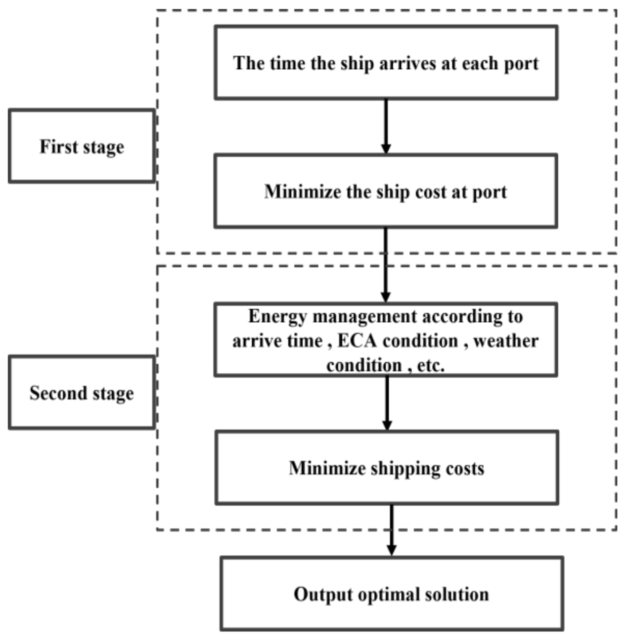
- We develop a two-stage optimization model to minimize the operational cost for a voyage. The first stage is optimizing the ships’ arrival time depending on the electricity price. In the second stage, we optimize ship speed and ESS energy usage, taking into account various factors such as ECA conditions, maritime meteorological conditions, and the cost of different fuels.
- (3)
- We conduct a comprehensive study to highlight how the proposed scheduling approach can effectively facilitate the voyage planning and energy interactions between the ship and shoreside OPS to improve the performance of a hybrid ship in terms of operation efficiency, electricity cost, and emission mitigation.
2. Model Formulation
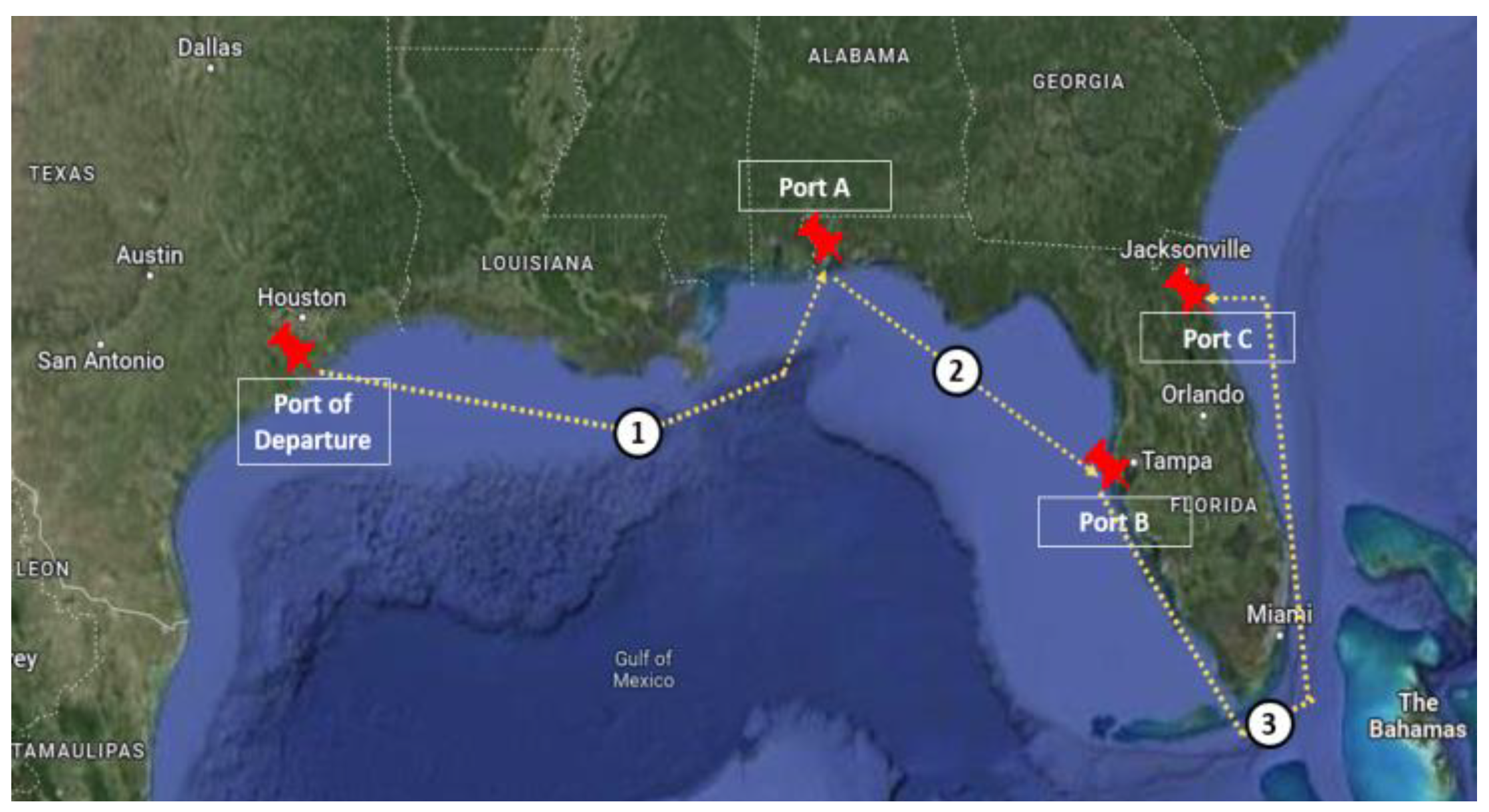
2.1. Voyage Scheduling
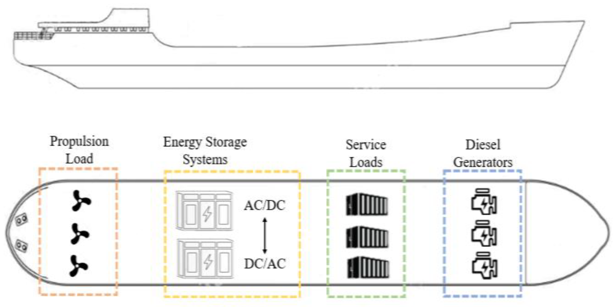
2.2. Energy Management
3. Numerical Analysis
3.1. Analysis of Navigation Optimization Results
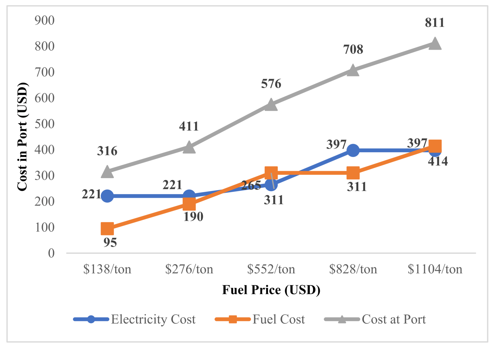
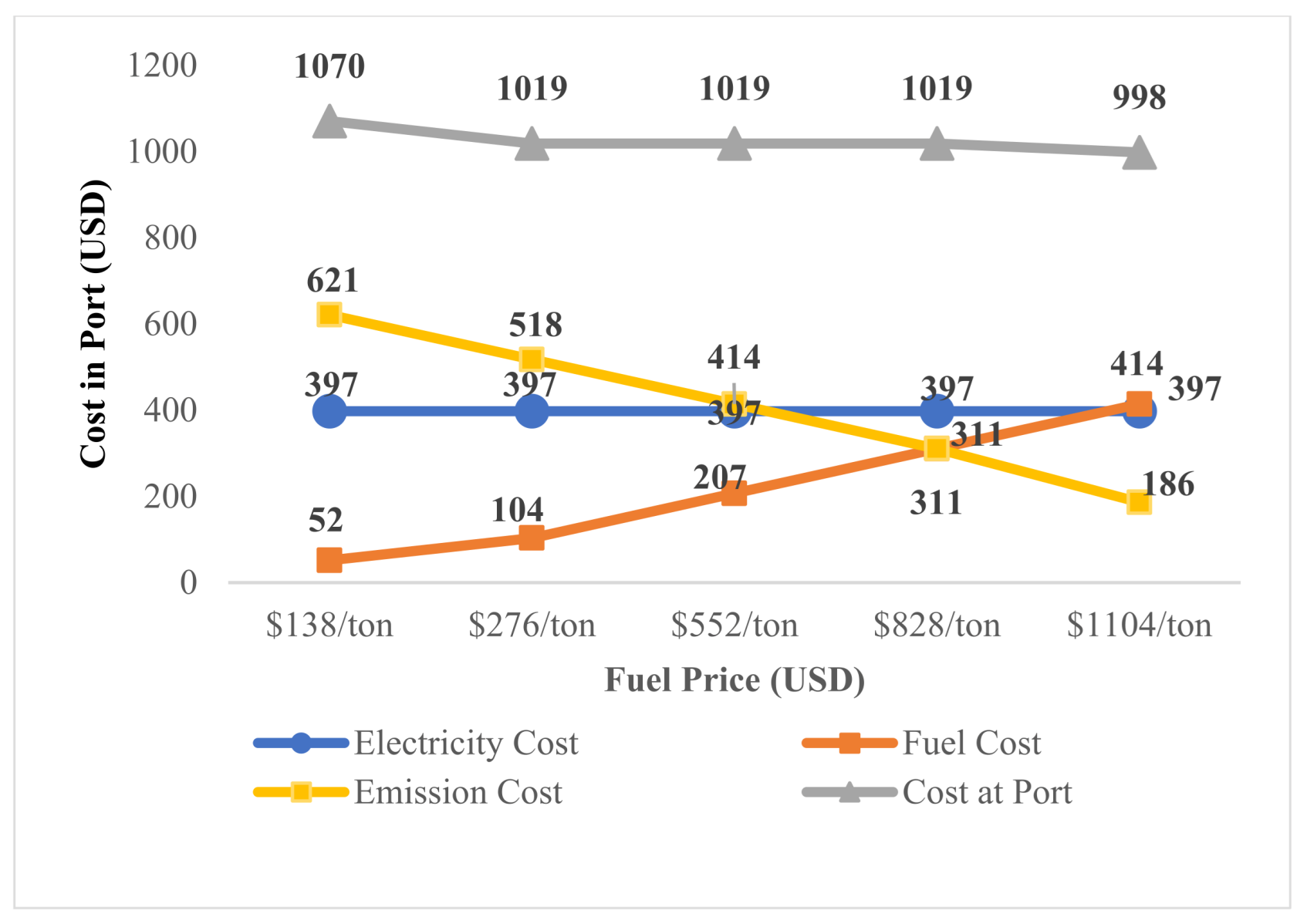
3.2. Sensitivity Analysis of Electricity Price
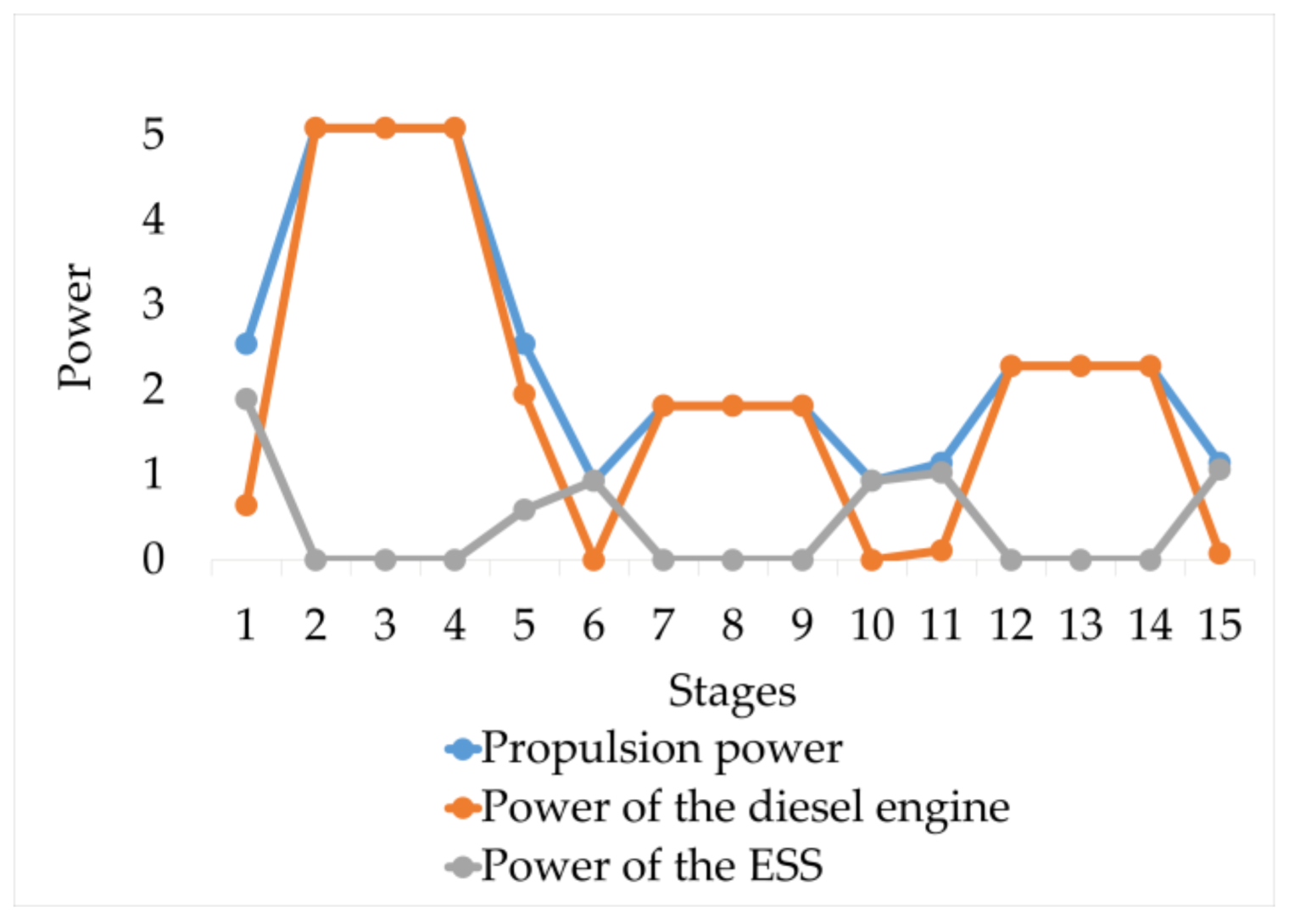
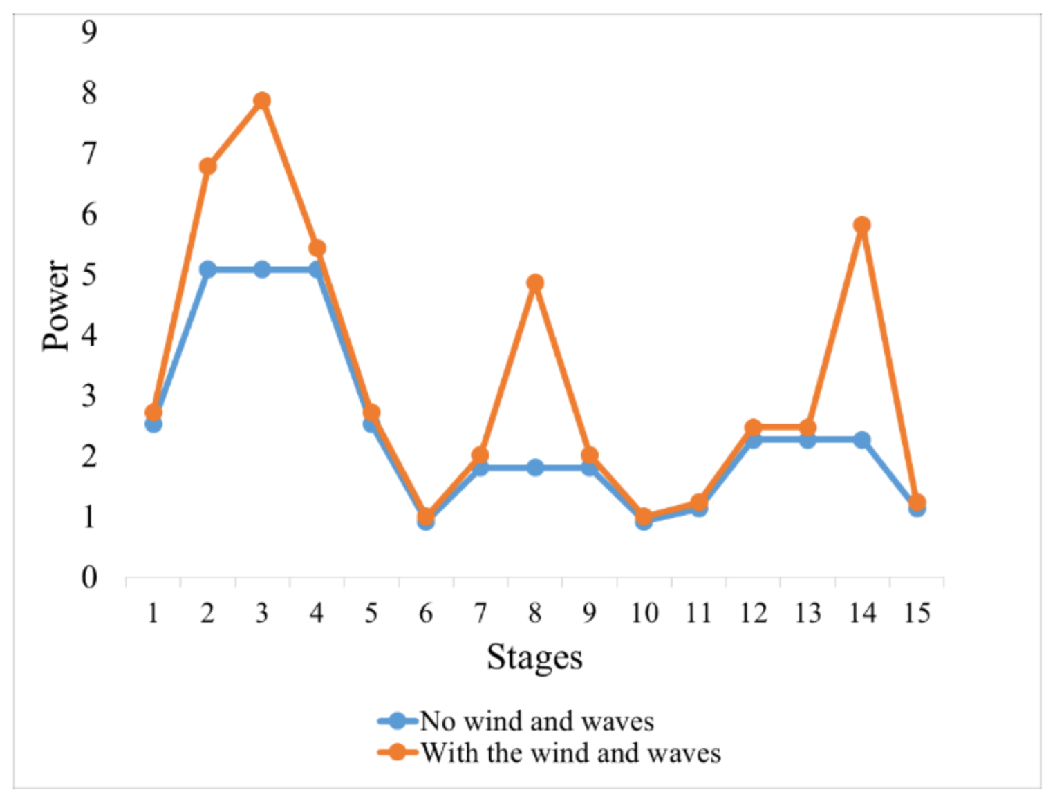
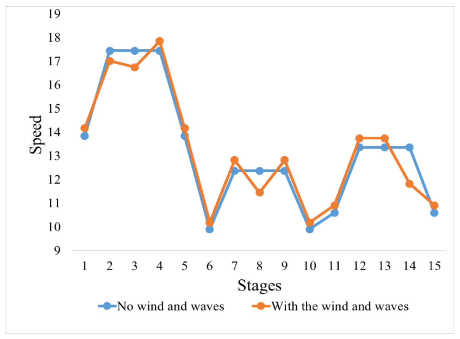
3.3. Analysis of Energy Management Results
3.4. Comparison of Jointed and Decouple Scheduling
4. Conclusions
Author Contributions
Funding
Institutional Review Board Statement
Informed Consent Statement
Data Availability Statement
Acknowledgments
Conflicts of Interest
References
- UNCTAD. Review of Maritime Transport 2019; United Nation Conference on Trade and Development: Geneva, Switzerland, 2019. [Google Scholar]
- IMO. Fourth Greenhouse Gas Study 2020. International Maritime Organization. Available online: https://www.imo.org/en/OurWork/Environment/Pages/Fourth-IMO-Greenhouse-Gas-Study-2020.aspx (accessed on 10 January 2023).
- IMO. Initial IMO GHG Strategy 2018. International Maritime Organization. Available online: https://www.imo.org/en/MediaCentre/HotTopics/Pages/Reducing-greenhouse-gas-emissions-from-ships.aspx (accessed on 10 January 2023).
- Esther, W. Your Climate Change Goals May Have a Maritime Shipping Problem. Available online: https://www.spglobal.com/esg/insights/your-climate-change-goals-may-have-a-maritime-shipping-problem (accessed on 10 January 2023).
- European Commission. Reducing Emissions from the Shipping Sector. 2021. Available online: https://ec.europa.eu/clima/eu-action/transport-emissions/reducing-emissions-shipping-sector_en (accessed on 10 January 2023).
- United Nations Climate Change Conference UK 2021. Clydebank Declaration For Green Shipping Corridors. Available online: https://ukcop26.org/cop-26-clydebank-declaration-for-green-shipping-corridors/ (accessed on 10 January 2023).
- Lindstad, E.; Eskeland, G.S.; Rialland, A.; Valland, A. Decarbonizing Maritime Transport: The Importance of Engine Technology and Regulations for LNG to Serve as a Transition Fuel. Sustainability 2020, 12, 8793. [Google Scholar] [CrossRef]
- Yuan, Y.P.; Wang, J.X.; Yan, X.P.; Shen, B.Y.; Long, T. A review of multi-energy hybrid power system for ships. Renew. Sustain. Energy Rev. 2020, 10, 110081. [Google Scholar] [CrossRef]
- Wienberg, C. Maersk Targets Bigger and Faster Cuts in Carbon Emissions. Available online: https://www.bloomberg.com/news/articles/2022-01-12/maersk-targets-bigger-and-faster-cuts-in-carbon-emissions (accessed on 10 January 2023).
- Ermakov, A. Natural Gas in the Transition to Low-Carbon Transport Systems: Focus on Marine Bunkering and NGVs. Available online: https://iaee2022.org/files/timetable/T000103_23_1.pdf (accessed on 10 January 2023).
- Inal, O.B.; Charpentier, J.F.; Deniz, C. Hybrid power and propulsion systems for ships: Current status and future challenges. Renew. Sustain. Energy Rev. 2022, 3, 111965. [Google Scholar] [CrossRef]
- Khan, M.M.S.; Faruque, M.O.; Newaz, A. Fuzzy Logic Based Energy Storage Management System for MVDC Power System of All Electric Ship. IEEE Trans. Energy Convers. 2017, 1, 798–809. [Google Scholar] [CrossRef]
- Bao, P.; Wang, W.T. Stability Improvement of Electric Ship Propulsion System Using Supercapacitor. J. Phys. Conf. Ser. 2021, 9, 012006. [Google Scholar] [CrossRef]
- Chen, H.; Zhang, Z.H.; Guan, C.; Gao, H.B. Optimization of sizing and frequency control in battery/supercapacitor hybrid energy storage system for fuel cell ship. Energy 2020, 3, 117285. [Google Scholar] [CrossRef]
- Hou, J.; Sun, J.; Hofmann, H. Control development and performance evaluation for battery/flywheel hybrid energy storage solutions to mitigate load fluctuations in all-electric ship propulsion systems. Appl. Energy 2018, 2, 919–930. [Google Scholar] [CrossRef]
- Jeong, H.W.; Ha, Y.S.; Kim, Y.S.; Kim, C.H.; Yoon, K.K.; Seo, D.H. Shore power to ships and offshore plants with flywheel energy storage system. J. Korean Soc. Mar. Eng. 2013, 11, 771–777. [Google Scholar] [CrossRef]
- Yu, Y.L.; Wang, Y.X.; Zhang, G.S.; Sun, F. Analysis of the comprehensive physical field for a new flywheel energy storage motor/generator on ships. J. Mar. Sci. Appl. 2012, 11, 134–142. [Google Scholar] [CrossRef]
- Jelić, M.; Mrzljak, V.; Radica, G.; Račić, N. An alternative and hybrid propulsion for merchant ships: Current state and perspective. Energy Sources Part A Recovery Util. Environ. Eff. 2021, 10, 1–33. [Google Scholar] [CrossRef]
- Zhang, Q.; Zheng, Z.Q.; Wan, Z.; Zheng, S.Y. Does emission control area policy reduce sulfur dioxides concentration in shanghai? Transp. Res. Part D Transp. Environ. 2020, 3, 102289. [Google Scholar] [CrossRef]
- Sun, Y.L.; Yang, L.X.; Zheng, J.F. Emission control areas: More or fewer? Transp. Res. Part D Transp. Environ. 2020, 7, 102349. [Google Scholar] [CrossRef]
- Li, L.Y.; Gao, S.X.; Yang, W.G.; Xiong, X. Ship’s response strategy to emission control areas: From the perspective of sailing pattern optimization and evasion strategy selection. Transp. Res. Part E Logist. Transp. Rev. 2019, 12, 101835. [Google Scholar] [CrossRef]
- Psaraftis, H.N.; Kontovas, C.A. Ship speed optimization: Concepts, models and combined speed-routing scenarios. Transp. Res. Part C Emerg. Technol. 2014, 7, 52–69. [Google Scholar] [CrossRef]
- Doudnikoff, M.; Lacoste, R. Effect of a speed reduction of containerships in response to higher energy costs in sulphur emission control areas. Transp. Res. Part D Transp. Environ. 2014, 5, 19–29. [Google Scholar] [CrossRef]
- Cariou, P.; Cheaitou, A. The effectiveness of a European speed limit versus an international bunker-levy to reduce CO2 emissions from container shipping. Transp. Res. Part D Transp. Environ. 2012, 3, 116–123. [Google Scholar] [CrossRef]
- Fagerholt, K.; Psaraftis, H.N. On two speed optimization problems for ships that sail in and out of emission control areas. Transp. Res. Part D Transp. Environ. 2015, 8, 56–64. [Google Scholar] [CrossRef]
- Wen, M.; Pacino, D.; Kontovas, C.A.; Psaraftis, H.N. A multiple ship routing and speed optimization problem under time, cost and environmental objectives. Transp. Res. Part D Transp. Environ. 2017, 5, 303–321. [Google Scholar] [CrossRef]
- Sun, B.; Niu, B.H.; Xu, H.F.; Ying, W.Z. Cooperative optimization for port and shipping line with unpredictable disturbance consideration. In Proceedings of the 2018 14th International Conference on Natural Computation, Fuzzy Systems and Knowledge Discovery (ICNC-FSKD), Huangshan, China, 28–30 July 2018; pp. 113–118. [Google Scholar]
- Zhang, Z.; Xu, G.P.; Li, X.H.; Zhu, T.L.; Fu, P. Analysis of shipping carbon reduction measures and the scenarios of shipping carbon reduction in China. Ind. Saf. Environ. Prot. 2021, 9, 63–69. [Google Scholar]
- Fagerholt, K.; Gausel, N.T.; Rakke, J.G.; Psaraftis, H.N. Maritime routing and speed optimization with emission control areas. Transp. Res. Part C Emerg. Technol. 2015, 3, 57–73. [Google Scholar] [CrossRef]
- Gan, L.X.; Lu, T.F.; Zheng, Y.Z.; Shu, Y.Q. Multi-objective optimization model of ship speed control for a route passing through eca. Navig. China 2020, 9, 15–19. [Google Scholar]
- Lin, G.H.; Gao, J.; Li, Y.W.; Xu, W.N. Optimization of liner routes and cargo allocation under eca and carbon tax policy. Ind. Eng. Manag. 2021, 5, 46–55. [Google Scholar]
- Balestra, L.; Schjølberg, I. Energy management strategies for a zero-emission hybrid domestic ferry. Int. J. Hydrogen Energy 2021, 11, 38490–38503. [Google Scholar] [CrossRef]
- Lan, H.; Wen, S.L.; Hong, Y.Y.; Yu, D.C.; Zhang, L.J. Optimal sizing of hybrid pv/diesel/battery in ship power system. Appl. Energy 2015, 11, 26–34. [Google Scholar] [CrossRef]
- Planakis, N.; Papalambrou, G.; Kyrtatos, N. Predictive power-split system of hybrid ship propulsion for energy management and emissions reduction. Control. Eng. Pract. 2021, 6, 104795. [Google Scholar] [CrossRef]
- Yi, H. Optimal operation strategy of a large fuel-cell hybrid ship. J. Adv. Mar. Eng. Technol. 2021, 8, 167–173. [Google Scholar] [CrossRef]
- Boveri, A.; Silvestro, F.; Molinas, M.; Skjong, E. Optimal sizing of energy storage systems for shipboard applications. IEEE Trans. Energy Convers. 2018, 11, 801–811. [Google Scholar] [CrossRef]
- Fang, S.D.; Xu, Y.; Li, Z.M.; Ding, Z.H.; Liu, L.; Wang, H.D. Optimal sizing of shipboard carbon capture system for maritime greenhouse emission control. IEEE Trans. Ind. Appl. 2019, 8, 5543–5553. [Google Scholar] [CrossRef]
- Vahabzad, N.; Mohammadi-Ivatloo, B.; Anvari-Moghaddam, A. Optimal energy scheduling of a solar-based hybrid ship considering cold-ironing facilities. IET Renew. Power Gener. 2021, 2, 532–547. [Google Scholar] [CrossRef]
- Wang, X.Z.; Shipurkar, U.; Haseltalab, A.; Polinder, H.; Claeys, F.; Negenborn, R.R. Sizing and control of a hybrid ship propulsion system using multi-objective double-layer optimization. IEEE Access 2021, 5, 72587–72601. [Google Scholar] [CrossRef]
- Zhang, M.; Tan, Z.J.; Gao, P.H. Optimizing Trajectory and Speed of Coastal Ship under Irregular ECA Boundary. J. Dalian Marit. Univ. 2023, 1, 1–11. [Google Scholar]
- Wen, S.L.; Zhao, T.Y.; Tang, Y.; Xu, Y.; Zhu, M.; Fang, S.D.; Ding, Z.H. Coordinated optimal energy management and voyage scheduling for all-electric ships based on predicted shore-side electricity price. IEEE Trans. Ind. Appl. 2020, 10, 139–148. [Google Scholar] [CrossRef]
- Shanghai Shipping Exchange. China Shipping Exchange Network. Available online: https://www.cn-eship.com/ (accessed on 3 March 2023).
- CNSS. China Maritime Service Network. Available online: https://www.cnss.com.cn/html/gkryjg (accessed on 3 March 2023).


| Indices | |
|---|---|
| Ports, = 1, …, K | |
| Stages, = 1, …, N | |
| Stages, = time, = 1, …, | |
| Parameters | |
| Number of ports | |
| Number of voyage stages | |
| Distance to port i in stage j of the ship | |
| Electricity price in the tth time period | |
| Fuel prices | |
| Fuel efficiency (Kg/KWh) | |
| Power required to load the ship at the ith port | |
| Gas emission coefficient | |
| Maximum sailing time | |
| Maximum speed of ship sailing | |
| Minimum speed of ship sailing | |
| Decision variables | |
| Whether the ship arrives at the ith port at time t | |
| Speed of the ship to the jth stage of the ith port | |
| Parameters | |
|---|---|
| Fuel price of stage of the ship going to the port. | |
| Coefficient of wind resistance. | |
| Coefficient of wave resistance. | |
| Coefficient of static water resistance. | |
| Maximum ESS operating power. | |
| Maximum operating power of diesel engine. | |
| ESS maximum energy storage. | |
| Charging time of the ship at the port. | |
| Water density. | |
| Air density. | |
| Variables | |
| Cost of the voyage of the ship to the stage of the port. | |
| Power of the ESS of the ship to the stage of the port. | |
| Power of the ship’s diesel engine to the stage of the port. | |
| Propulsion power of the ship to the stage of the port. | |
| Port of Departure | Segment | ECA Inside/n Mile | ECA Outside/n Mile |
|---|---|---|---|
| A | 1 | 50 | 0 |
| 2 | 0 | 68 | |
| 3 | 0 | 55 | |
| 4 | 0 | 60 | |
| 5 | 40 | 0 | |
| B | 6 | 40 | 0 |
| 7 | 0 | 60 | |
| 8 | 0 | 87 | |
| 9 | 0 | 56 | |
| 10 | 45 | 0 | |
| C | 11 | 45 | 0 |
| 12 | 0 | 82 | |
| 13 | 0 | 63 | |
| 14 | 0 | 55 | |
| 15 | 40 | 0 |
| Ship Parameters | Numerical Value |
|---|---|
| Size of ship/m | 98 × 16 |
| Carrying capacity/ton | 5000 |
| Number of diesel engines | 2 |
| Maximum operating power of diesel engine/MWh | 6 |
| Maximum ESS operating power/MW | 2 |
| ESS maximum energy storage/MW | 8 |
| Charging efficiency | 1 |
| Load efficiency | 2 |
| Maximum sailing time /h | 100 |
| Speed limit [Min, Max]/(n mile/h) | [5, 25] |
| Berthing time in each port/h | [8,8,8] |
| Charge time for each port ESS/h | [8,8,8] |
| Fuel Type | Fuel Price (USD)/t | Cost at Port (USD) | Fuel Cost (USD) | Emission Cost (USD) |
|---|---|---|---|---|
| HFO | 138 | 1070.27 | 17.25 | 207.02 |
| IFO180 | 276 | 1018.51 | 34.50 | 172.51 |
| IFO380 | 552 | 1018.51 | 69.01 | 138.01 |
| MDO | 828 | 1018.51 | 103.51 | 103.51 |
| MGO | 1104 | 915.01 | 138.01 | 34.50 |
| Ship Leaves at 12 a.m. | Ship Leaves at 6 a.m. | Ship Leaves at 12 p.m. | Ship Leaves at 6 p.m. | |||||
|---|---|---|---|---|---|---|---|---|
| Time of Arrival (24 h) | Voyage Time (h) | Time of Arrival (24 h) | Voyage Time (h) | Time of Arrival (24 h) | Voyage Time (h) | Time of Arrival (24 h) | Voyage Time (h) | |
| Port A | 17 | 17 | 17 | 17 | 6 | 30 | 5 | 29 |
| Port B | 18 | 15 | 8 | 29 | 8 | 16 | 5 | 14 |
| Port C | 17 | 13 | 8 | 14 | 7 | 13 | 5 | 14 |
| Ports | Segment | ECA Inside/Outside | Speed (n mile/h) | Sailing Time (h) | Propulsion Power (MW) | Diesel Engine Power (MW) | ESS Power (MW) | ESS Service Time (h) | Reserve Service Time (h) | Fuel Costs (USD) |
|---|---|---|---|---|---|---|---|---|---|---|
| A | 1 | ECA Inside | 13.84 | 3.61 | 2.54 | 0.65 | 1.90 | 3.61 | 0.00 | 531.75 |
| 2 | ECA Outside | 17.44 | 3.90 | 5.09 | 5.09 | 0.00 | 0.00 | 0.00 | 2190.90 | |
| 3 | ECA Outside | 17.44 | 3.16 | 5.09 | 5.09 | 0.00 | 0.00 | 0.00 | 1772.03 | |
| 4 | ECA Outside | 17.44 | 2.44 | 5.09 | 5.09 | 0.00 | 0.00 | 0.00 | 1933.14 | |
| 5 | ECA Inside | 13.84 | 2.89 | 2.54 | 0.65 | 0.59 | 1.94 | 0.95 | 1355.11 | |
| B | 6 | ECA Inside | 9.90 | 4.04 | 0.93 | 0.00 | 0.93 | 4.04 | 0.00 | 0.00 |
| 7 | ECA Outside | 12.37 | 4.85 | 1.82 | 1.82 | 0.00 | 0.00 | 0.00 | 972.55 | |
| 8 | ECA Outside | 12.37 | 7.04 | 1.82 | 1.82 | 0.00 | 0.00 | 0.00 | 1410.18 | |
| 9 | ECA Outside | 12.37 | 4.53 | 1.82 | 1.82 | 0.00 | 0.00 | 0.00 | 907.72 | |
| 10 | ECA Inside | 9.90 | 4.55 | 0.93 | 0.00 | 0.93 | 4.55 | 0.00 | 0.00 | |
| C | 11 | ECA Inside | 10.60 | 4.25 | 1.14 | 0.11 | 1.03 | 4.11 | 0.14 | 340.71 |
| 12 | ECA Outside | 13.35 | 6.14 | 2.29 | 2.29 | 0.00 | 0.00 | 0.00 | 1291.19 | |
| 13 | ECA Outside | 13.35 | 4.72 | 2.29 | 2.29 | 0.00 | 0.00 | 0.00 | 992.01 | |
| 14 | ECA Outside | 13.35 | 4.12 | 2.29 | 2.29 | 0.00 | 0.00 | 0.00 | 866.04 | |
| 15 | ECA Inside | 10.60 | 3.78 | 1.14 | 0.11 | 1.07 | 3.53 | 0.24 | 793.56 | |
| Total Fuel Consumption Cost: 15,356.89 | ||||||||||
| Port of Departure | Segment | ECA Inside/Outside | Wind Speed (Knot) | Wave Speed (Knot) |
|---|---|---|---|---|
| A | 1 | ECA inside | 0 | 0 |
| 2 | ECA outside | 2 | 2 | |
| 3 | ECA outside | 3 | 5 | |
| 4 | ECA outside | 0 | 0 | |
| 5 | ECA inside | 0 | 0 | |
| B | 6 | ECA inside | 0 | 0 |
| 7 | ECA outside | 0 | 0 | |
| 8 | ECA outside | 5 | 6 | |
| 9 | ECA outside | 0 | 0 | |
| 10 | ECA inside | 0 | 0 | |
| C | 11 | ECA inside | 0 | 0 |
| 12 | ECA outside | 0 | 0 | |
| 13 | ECA outside | 0 | 0 | |
| 14 | ECA outside | 6 | 4 | |
| 15 | ECA inside | 0 | 0 |
| Ports | Segment | ECA Inside/Outside | Speed (n mile/h) | Sailing Time (h) | Propulsion Power (MW) | Diesel Engine Power (MW) | ESS Power (MW) | ESS Service Time (h) | Reserve Service Time (h) | Costs (USD) |
|---|---|---|---|---|---|---|---|---|---|---|
| A | 1 | ECA Inside | 14.16 | 3.53 | 2.73 | 1.45 | 1.28 | 3.34 | 0.19 | 1181.42 |
| 2 | ECA Outside | 17.01 | 4.00 | 6.80 | 6.00 | 0.80 | 0.00 | 4.00 | 2999.07 | |
| 3 | ECA Outside | 16.76 | 3.29 | 7.89 | 6.00 | 1.89 | 0.00 | 3.29 | 2860.80 | |
| 4 | ECA Outside | 17.84 | 3.36 | 5.45 | 5.45 | 0.00 | 0.00 | 0.00 | 2024.82 | |
| 5 | ECA Inside | 14.16 | 2.82 | 2.73 | 1.04 | 1.69 | 2.21 | 0.62 | 878.75 | |
| B | 6 | ECA Inside | 10.18 | 3.93 | 1.01 | 0.02 | 0.99 | 3.86 | 0.07 | 36.27 |
| 7 | ECA Outside | 12.82 | 4.68 | 2.02 | 2.02 | 0.00 | 0.00 | 0.00 | 1045.45 | |
| 8 | ECA Outside | 11.45 | 7.60 | 4.87 | 4.87 | 0.00 | 0.00 | 0.00 | 4087.44 | |
| 9 | ECA Outside | 12.82 | 4.37 | 2.02 | 2.02 | 0.00 | 0.00 | 0.00 | 975.77 | |
| 10 | ECA Inside | 10.18 | 4.42 | 1.01 | 0.02 | 0.99 | 4.24 | 0.19 | 63.22 | |
| C | 11 | ECA Inside | 10.91 | 4.13 | 1.25 | 0.20 | 1.05 | 3.42 | 0.70 | 344.56 |
| 12 | ECA Outside | 13.74 | 5.97 | 2.49 | 2.49 | 0.00 | 0.00 | 0.00 | 1640.75 | |
| 13 | ECA Outside | 13.74 | 4.59 | 2.49 | 2.49 | 0.00 | 0.00 | 0.00 | 1260.59 | |
| 14 | ECA Outside | 11.82 | 4.65 | 5.83 | 5.83 | 0.00 | 0.00 | 0.00 | 2996.82 | |
| 15 | ECA Inside | 10.91 | 3.67 | 0.03 | 0.03 | 1.21 | 3.65 | 0.02 | 31.77 | |
| Total Fuel Consumption Cost: 22,427.51 | ||||||||||
| Decoupled Scheduling | Proposed Joint Scheduling | Cost Reduction | |
|---|---|---|---|
| Cost in port (USD) | 1004.19 | 915.01 | 8.88% |
| Voyage cost (USD) | 24,582.84 | 22,427.51 | 8.77% |
| Total cost (USD) | 25,587.03 | 23,342.52 | 8.77% |
Disclaimer/Publisher’s Note: The statements, opinions and data contained in all publications are solely those of the individual author(s) and contributor(s) and not of MDPI and/or the editor(s). MDPI and/or the editor(s) disclaim responsibility for any injury to people or property resulting from any ideas, methods, instructions or products referred to in the content. |
© 2023 by the authors. Licensee MDPI, Basel, Switzerland. This article is an open access article distributed under the terms and conditions of the Creative Commons Attribution (CC BY) license (https://creativecommons.org/licenses/by/4.0/).
Share and Cite
Wang, Y.; Liang, C.; Aktas, T.U.; Shi, J.; Pan, Y.; Fang, S.; Lim, G. Joint Voyage Planning and Onboard Energy Management of Hybrid Propulsion Ships. J. Mar. Sci. Eng. 2023, 11, 585. https://doi.org/10.3390/jmse11030585
Wang Y, Liang C, Aktas TU, Shi J, Pan Y, Fang S, Lim G. Joint Voyage Planning and Onboard Energy Management of Hybrid Propulsion Ships. Journal of Marine Science and Engineering. 2023; 11(3):585. https://doi.org/10.3390/jmse11030585
Chicago/Turabian StyleWang, Yu, Chengji Liang, Tugce Uslu Aktas, Jian Shi, Yang Pan, Sidun Fang, and Gino Lim. 2023. "Joint Voyage Planning and Onboard Energy Management of Hybrid Propulsion Ships" Journal of Marine Science and Engineering 11, no. 3: 585. https://doi.org/10.3390/jmse11030585
APA StyleWang, Y., Liang, C., Aktas, T. U., Shi, J., Pan, Y., Fang, S., & Lim, G. (2023). Joint Voyage Planning and Onboard Energy Management of Hybrid Propulsion Ships. Journal of Marine Science and Engineering, 11(3), 585. https://doi.org/10.3390/jmse11030585