Node Depth Adjustment Based Target Tracking in Sparse Underwater Sensor Networks

Abstract

Due to the limited energy in underwater sensor networks, underwater nodes need to be deployed sparsely. However, sparse USNs will lead to poor tracking coverage and detection capability. To solve these problems, the mobility of nodes in depth can be utilized to optimize the node topology to achieve data fusion more reliably and effectively. In this paper, for underwater target tracking, a node depth adjustment algorithm is proposed. Firstly, after introducing the sound velocity profile on acoustic signal transmission, the asynchronous particle filter algorithm based on delay estimation is improved, which makes the filter more suitable for an underwater environment. Secondly, the influence of node topology on the tracking accuracy is analyzed, and the optimization problem of node depth adjustment is constructed, in which the depth-related Fisher Information Matrix is designed as the optimization criterion. Thirdly, for scenarios in which the target depth is either known or unknown, the analytical method and the interior point method are employed to solve the problem, respectively, and the optimal depth adjustment strategies in corresponding scenarios are obtained. The simulation results show that the proposed algorithm can fully adjust the node depth and achieve a more accurate tracking performance.

1. Introduction

The ocean, which occupies 71% of the earth’s area, is rich in natural resources and strategic status. As a necessary technology for underwater defense and resource development, underwater target tracking has received extensive attention and research in recent years [1,2,3]. With the rapid development of wireless sensor networks, underwater target tracking based on underwater sensor networks (USNs) has also received extensive attention [4,5,6]. Unlike traditional acoustic sensor arrays [7] or acoustic imaging sensors [8], USNs have the advantage of flexible distribution, comprehensive dimensions and strong concealment, which allow them to achieve better real-time tracking [9]. In this paper, we focus on solving the problem of underwater target tracking using USNs.

To track the moving targets, underwater sensor nodes with sensing ability are needed to collect measurements and transmit data related. Too few nodes participating in tracking will lead to fewer measurements and increase the tracking error; while more nodes will cause data redundancy and create unnecessary waste [10]. Therefore, how to effectively balance the number of nodes participating in tracking and the tracking accuracy is an urgent problem to be solved. To this end, researchers have proposed a large number of solutions from multiple perspectives. After improving the particle filter with the help of mutual information (MI), ref. [11] presents a node scheduling strategy based on posterior Cramer–Rao lower bound (PCRLB) to improve the tracking efficiency [11]. Ref. [12] sets three indicators as the objective function to design a multi-objective node selection algorithm, which overcomes the influence of node position fluctuations and achieves better performance. Zhang S designs an unbiased quantizer and achieves optimal bit allocation, which reduces the number of nodes and the amount of measurement involved in tracking [13]. The relationship between node topology and PCRLB is derived in [14], and it also improves tracking accuracy by selecting a specific topology. Xu S [15] studied the optimal sensor deployment strategy for 3D-AOA localization combined with topology. The studies above are based on USNs in which underwater nodes are deployed densely. However, considering the relevant high cost of underwater sensor nodes, it is difficult to deploy them as densely as wireless sensor networks [16,17]. At the same time, the dense deployment of nodes will cause collisions and packet loss [18]. Therefore, we have to sparsely deploy nodes in the underwater area.

However, sparse USNs will lead to poor tracking coverage and detection capability. Once the target moves to an area with low coverage, USNs cannot obtain enough data due to the limitation of the node sensing radius. A feasible way to solve the above problems is to use the mobility of nodes. The authors of [19] set a mobile sink as the relay node to balance the energy consumption of each node during data gathering. Ref. [20] constructed a node scheduling and depth adjustment algorithm using the theory of two-dimensional convex hull and spanning tree to obtain higher network coverage. For wireless sensor networks, considering the mobility of nodes, ref. [21] obtained the optimal combination of nodes through an optimization algorithm to improve tracking accuracy. An Autonomous Underwater Vehicle was introduced into [22]; its fusion center can be moved to the optimal position to reduce the energy consumption of nodes during acoustic communication. However, these mobility policies do not actually apply to USNs. It is difficult to move the sensor nodes to any given location. Underwater sensor nodes are usually equipped with pressure monitors which can flexibly change the depth by using pressure. Therefore, node depth adjustment becomes an easier solution. Ref. [23] realizes the self-organized adjustment of the node position structure through the dynamic adjustment of the node depth, which improves the tracking accuracy. Ref. [24] combines node selection with depth adjustment, which enhanced the real time performance of the algorithm while reducing the tracking error. However, the algorithm mentioned above does not take the impact of node topology on tracking into account, so there are certain defects.

In recent years, as the application background of target tracking has become more and more complex, the tracking scenarios are no longer limited to ideal environments [25,26,27]. In reality, underwater acoustic transmission generally has problems such as large delay, small bandwidth, serious clutter and scattering. Another of these issues is the transmission speed of the sound wave underwater at 1480 m/s, presenting a larger propagation delay and asynchronous phenomenon than the land scene [28]. To solve this problem, ref. [29] proposed a Kalman filter and a particle filter based on sequential asynchronous filters, which overcome the disadvantage that the asynchronous measurement cannot be directly fused. Ref. [30] establishes the relationship between snapshot state and asynchronous measurements and designs an asynchronous particle filter algorithm based on delay estimation. However, in addition to the propagation delay, the underwater environment also has a depth-dependent sound velocity profile phenomenon. None of the articles above considered the acoustic ray transmission.

In summation, in the field of underwater target tracking, research on node mobility has achieved many results. However, there are still research gaps in the problem of node depth considering a complex underwater environment. Therefore, in order to solve the problems of underwater sensor transmission delay and node topology in the process of node depth adjustment, this paper studies the node depth adjustment in sparse underwater sensor networks through the convex optimization.

The main original work includes:

• Considering the transmission delay and sound velocity profile theory, the particle filter algorithm under time delay estimation is improved;
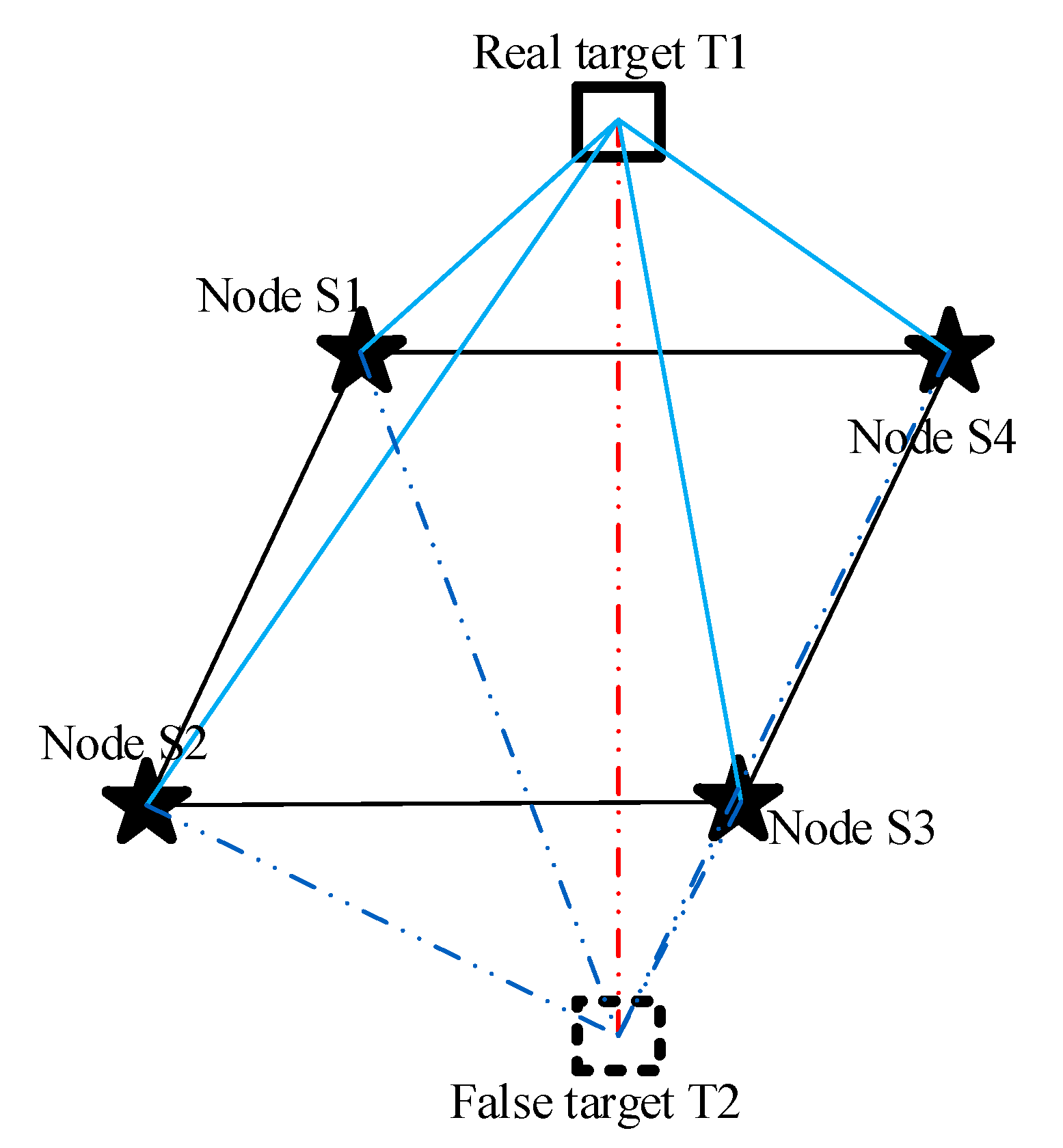
• The problem of depth adjustment is constructed. Based on the relationship between FIM and node depth, the problem above is converted into an optimization problem. To avoid the impact of the four-point coplanar topology on tracking and positioning, the node topology constraint is also designed;
• A node depth adjustment algorithm using convex optimization is proposed, different solution strategies are designed for cases in which the target depth is known or unknown, and the node depth adjustment is realized.

The rest of the paper proceeds as follows. In Section 2, the system model is formulated and the particle filter under time delay estimation is also improved. After deriving the relationship between node depth and FIM, a node depth adjustment problem considering topology is designed in Section 3. In Section 4, the corresponding algorithms are proposed when the target depth is known and unknown. In Section 5, simulation results are presented to verify the effectiveness of our algorithm. Finally, the conclusions of this paper are drawn in Section 6.

2. System Model

2.1. Target State Model

In this paper, the target is assumed to perform a constant velocity (CV) movement in the underwater three-dimensional space. For the sake of simplicity, a maneuvering point is used to model this target. The target state can be expressed as:

$$\begin{array}{c}{\mathit{X}}_{\mathit{k}}={\mathit{F}}_{\mathit{k}-1}{\mathit{X}}_{\mathit{k}-1}+{\omega }_{\mathit{k}-1}\end{array}$$

(1)

where ${\mathit{X}}_{\mathit{k}}={\left[x_k,{\dot{x}}_k,y_k,{\dot{y}}_k,z_k,{\dot{z}}_k\right]}^T$ is the target state at time k. The real position and velocity vector of the target in each direction is given by ${\mathit{u}}_k={\left[x_k,y_k,z_k\right]}^T$ and ${\mathit{v}}_k={\left[{\dot{x}}_k,{\dot{y}}_k,{\dot{z}}_k\right]}^T$, respectively. The state transition matrix is given as:

$$\begin{array}{l}{\mathit{F}}_{k-1}=diag\left({\mathit{F}}_{CV},{\mathit{F}}_{CV},{\mathit{F}}_{CV}\right)\\ {\mathit{F}}_{CV}=\left[\begin{array}{cc}1& T\\ 0& 1\end{array}\right]\end{array}$$

(2)

where $diag(\cdot )$ means a diagonal matrix, T is the sampling interval. The process noise ${\mathit{\omega }}_{\mathit{k}-1}$ is assumed to be the white, zero-mean and Gaussian with the covariance matrix ${\mathit{Q}}_{\mathit{k}-1}$:

$$\begin{array}{l}{\mathit{Q}}_{\mathit{k}-1}=q^{2}diag\left(\mathit{Q}\mathit{,}\mathit{Q}\mathit{,}\mathit{Q}\right)\\ \mathit{Q}=\left[\begin{array}{cc}\frac{T^3}{3}& \frac{T^2}{2}\\ \frac{T^2}{2}& T\end{array}\right]\end{array}$$

(3)

where $q^2$ means the process noise parameter.

Sound travels relatively slowly in an underwater environment compared to radio in the air. In sparse underwater sensor networks, the nodes are sparsely deployed and widely distributed. It is difficult to obtain synchronous measurements of the target; at the same time, the impact of transmission delay cannot be ignored. Typically, the transmission delay is affected by propagation speed and transmission time [31]. The propagation speed of underwater sound is different in environments with different salinity and temperature, and at different depths. During target tracking, the temperature and salinity of the monitoring area are basically stable, and only the propagation depth is constantly changed by the movement of the target and underwater sensor nodes. Therefore, we assume that the temperature and salinity are fixed, and mainly consider the effect of depth change on sound velocity.

As shown in Figure 1, under the influence of transmission delay, there is a significant difference between the target position at the sampling moment and the real position corresponding to the measurement. Therefore, the transmission delay is introduced into the target state model. Considering the ray tracing and depth-dependent sound velocity profile [32] as shown in Figure 2, the transmission delay ${\tau }_{b,n}$ between the target and the sensor node can be expressed as:

$${\tau }_{b,n}=-\frac{1}{\overline{a}}\left(\ln \frac{1+\sin {\theta }_b}{\cos {\theta }_b}-\ln \frac{1+\sin {\theta }_n}{\cos {\theta }_n}\right)$$

(4)

where $\overline{a}$ is the update factor, ${\theta }_b={\beta }_0-{\alpha }_0$ and ${\theta }_n={\beta }_0+{\alpha }_0$ represent the ray angle at the target and the nth node, respectively; ${\beta }_0=\arctan \left(\frac{z_k-z_k^n}{\sqrt{{\left(x_k-x_k^n\right)}^2+{\left(y_k-y_k^n\right)}^2}}\right)$ represents the angle of the straight line between target and the nth node; ${\alpha }_0=\frac{0.5\overline{a}\sqrt{{\left(x_k-x_k^n\right)}^2+{\left(y_k-y_k^n\right)}^2}}{\overline{b}+0.5\overline{a}\left(z_k-z_k^n\right)}$ represents the angle of the ray trajectory deviates from this straight line; $\overline{b}$ is the speed of sound.

After computing the transmission delay ${\tau }_{b,n}$, the real state corresponding to the measurement in (1) is given as:

$$\begin{array}{c}{X}_{t_k^i}=\left[\begin{array}{c}{x}_{t_k^i}\\ {\dot{x}}_{t_k^i}\\ y_{t_k^i}\\ {\dot{y}}_{t_k^i}\\ z_{t_k^i}\\ {\dot{z}}_{t_k^i}\end{array}\right]\end{array}=\left[\begin{array}{c}{x}_k-{\dot{x}}_k{\tau }_{b,n}\\ {\dot{x}}_k\\ y_k-{\dot{y}}_k{\tau }_{b,n}\\ {\dot{y}}_k\\ z_k-{\dot{z}}_k{\tau }_{b,n}\\ {\dot{z}}_k\end{array}\right]$$

(5)

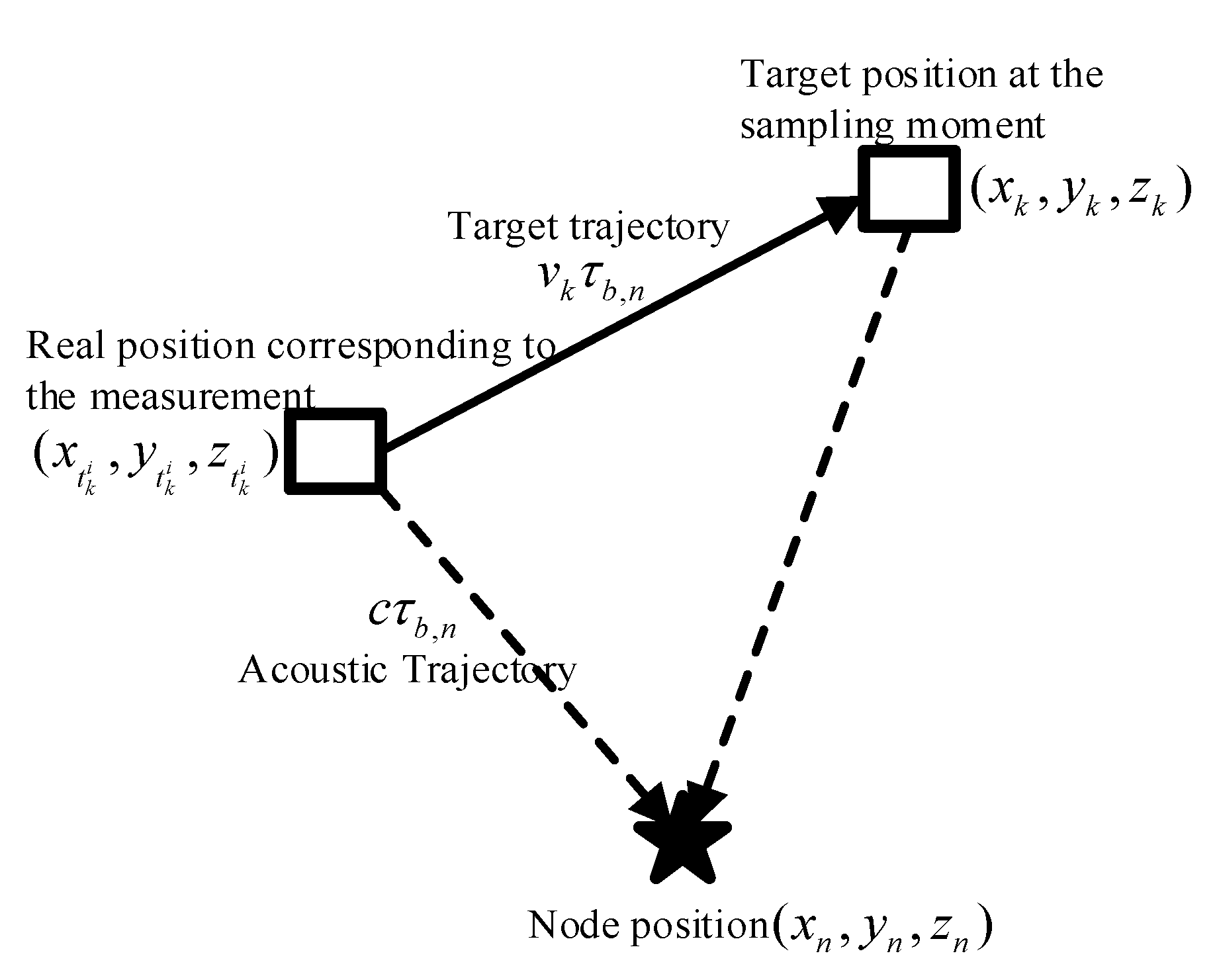
2.2. Measurement Model

We assume M = 4 underwater sensor nodes are placed in the sparse USNs, and that they send acoustic waves and compute the range measurements via the time of arrival (TOA) algorithm [33]. As shown in [33], based on the TOA of echoes from the target after transmitting acoustic pulses from the nodes, the ranges of the nodes to the target are determined. To simplify the problem and find out the rules of node depth adjustment, we assume the detection model of nodes satisfies the 0–1 model [34], so there is no possibility of locating incorrect targets. The range measurement of the nth node at time k is:

$$\begin{array}{c}{Z}_k^n=h_k^n\left({\mathit{X}}_{\mathit{k}}\right)+v_k^n\end{array}$$

(6)

$$\begin{array}{c}{h}_k^n\left({\mathit{X}}_{\mathit{k}}\right)=r_n\left(k\right)=\sqrt{{\left(x_k-x_k^n\right)}^2+{\left(y_k-y_k^n\right)}^2+{\left(z_k-z_k^n\right)}^2}\end{array}$$

(7)

where $Z_k^n$ is the range measurement of the nth node at time k; $h_k^n\left({\mathit{X}}_{\mathit{k}}\right)$ represents the measurement equation; ${\mathit{s}}_{\mathit{k}}^{\mathit{n}}={\left[x_k^n,y_k^n,z_k^n\right]}^T\left(n=1,\cdots ,M\right)$ is the real position of the nth node; $v_k^n$ is the measurement noise, which is assumed to be independent and follows a Gaussian distribution with parameters $N\left(0,{\sigma }_v^2\right)$.

As shown in Figure 2, the transmission of sound is not a straight line but a curve due to the sound velocity profile. After taking this into consideration, a coefficient is needed to correct the range measurement of (6). So, multiplicative noise is used to represent the correction coefficient, and (6) can be further expressed as:

$$\begin{array}{c}{Z}_k^n=\left(1+{\delta }_k^n\right)h_k^n\left({\mathit{X}}_{\mathit{k}}\right)+v_k^n\end{array}$$

(8)

where ${\delta }_k^n$ is the multiplicative noise which satisfies ${\delta }_k^n~N\left(0,{\sigma }_{\delta }^2\right)$ and $v_k^n$ is regarded as the additive noise. In this case, ${\zeta }_k^n$ is the measurement noise of the nth node at time k, i.e., ${\zeta }_k^n\sim N\left(0,r_n\left(k\right){\delta }_k^n+v_k^n\right)$.

2.3. Improved Particle Filter under Time Delay Estimation

Considering the nonlinear characteristic of (8), the particle filter (PF) is used to realize data fusion. PF can solve the nonlinear and non-Gaussian problems of underwater target tracking [35,36]. To overcome the defects in calculation of transmission delay in [30], (4) is introduced to improve the algorithm, which makes the proposed particle filter algorithm more suitable for underwater scenes.

Assuming the probability density function (pdf) of each node at time k is $p\left(Z_k^n|{\mathit{x}}_{\mathit{k}}^{\mathit{i}}\right)$, the measurement likelihood over all M nodes is given by:

$$\begin{array}{c}p\left({\mathit{{\rm Z}}}_{\mathit{\kappa }}|{\mathit{x}}_{\mathit{k}}^{\mathit{i}}\right)={{\displaystyle \prod }}_{n=1}^{M}p\left(Z_k^n|{\mathit{x}}_{\mathit{k}}^{\mathit{i}}\right)\end{array}$$

(9)

where ${\mathit{Z}}_{\mathit{k}}=\left(Z_k^1,Z_k^2,\cdots ,Z_k^M\right)$. After adopting the transition prior $p\left({\mathit{x}}_{\mathit{k}}|{\mathit{x}}_{\mathit{k}-1}\right)$ as the proposal distribution, the importance weights of particles are calculated as:

$$\begin{array}{c}{\omega }_k^i={\omega }_{k-1}^{i}p\left(Z_k|{\mathit{x}}_{\mathit{k}}^{\mathit{i}}\right)\end{array}$$

(10)

The specific process is shown in Algorithm 1.

Algorithm 1. Improved particle filter under time delay estimation.

Obtain the sampled particles ${\mathit{x}}_{\mathit{k}}^{\mathit{i}}$ based on the prior state $p\left({\mathit{x}}_{\mathit{k}-1}\right)$ 1. for $i=1\cdots M$ do 2.     Calculate the transmission delay by (4); 3.     Calculate the real state corresponding to the measurement by (5); 4.     Calculate the likelihood function; 5. end for 6. Update importance weights by (10) 7. Normalize the weight using ${\omega }_k^i={\omega }_k^i/{{\displaystyle \sum }}_{i=1}^N{\omega }_k^i$ 8. Estimate out the target state ${\widehat{\mathit{x}}}_{\mathit{k}}={{\displaystyle \sum }}_{i=1}^N{\omega }_k^i{\mathit{x}}_{\mathit{k}}$ 9. Resampling $\left\{{\mathit{x}}_{\mathit{k}}^{\mathit{i}},N^{-1}\right\}~\left\{{\mathit{x}}_{\mathit{k}}^{\mathit{i}},{\omega }_k^i\right\}$

3. Problem Formulation

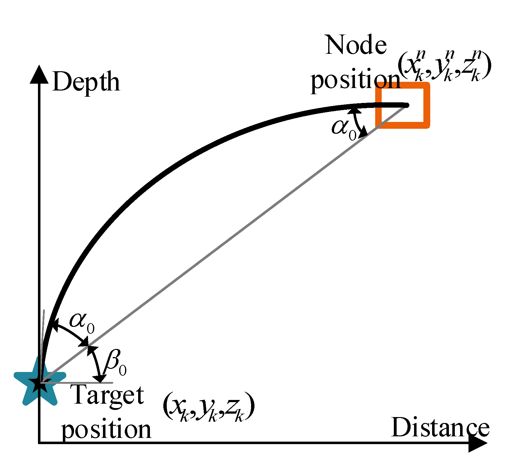
3.1. Relationship between FIM and Node Depth

The Fisher Information Matrix (FIM) provides a theoretical limit on the mean square error (MSE) of target state estimation during tracking, which is represented as [37]:

$$\begin{array}{c}E\left[{\widehat{\mathit{X}}}_{\mathit{k}}-{\mathit{X}}_{\mathit{k}}\right]{\left[{\widehat{\mathit{X}}}_{\mathit{k}}-{\mathit{X}}_{\mathit{k}}\right]}^T\ge {\mathit{J}}_{\mathit{k}}^{-1}\end{array}$$

(11)

where E express the expectation, ${\widehat{\mathit{X}}}_{\mathit{k}}$ is the estimate of ${\mathit{X}}_{\mathit{k}}$, and ${\mathit{J}}_{\mathit{k}}$ is the FIM at kth time. ${\mathit{J}}_{\mathit{k}}$ can be calculated as:

$$\begin{array}{c}{\mathit{J}}_{\mathit{k}}=E_{p\left({\mathit{Z}}_k,{\mathit{X}}_k|{\mathit{Z}}_{1:k-1}\right)}\end{array}\left[-{\nabla }_{{\mathit{X}}_k}^{{\mathit{X}}_k}\log p\left({\mathit{Z}}_{\mathit{k}},{\mathit{X}}_{\mathit{k}}|{\mathit{Z}}_{1\mathit{:}k-1}\right)\right]$$

(12)

where ${\nabla }_{{\mathit{X}}_k}^{{\mathit{X}}_k}={\nabla }_{{\mathit{X}}_k}{\nabla }_{{\mathit{X}}_k}^T$ is the second-order partial derivative operator with respect to ${\mathit{X}}_{\mathit{k}}$. $E_{\mathit{a}}[\cdot ]$ denote the expectation with respect to a.

Since $p\left({\mathit{Z}}_{\mathit{k}},{\mathit{X}}_{\mathit{k}}|{\mathit{Z}}_{\mathit{1}\mathit{:}\mathit{k}\mathbf{-}\mathbf{1}}\right)=p\left({\mathit{Z}}_{\mathit{k}}|{\mathit{X}}_{\mathit{k}}\right)p\left({\mathit{X}}_{\mathit{k}}|{\mathit{Z}}_{\mathit{1}\mathit{:}\mathit{k}-\mathit{1}}\right)$, (12) can be decomposed into two parts as [38]:

$$\begin{array}{c}{\mathit{J}}_{\mathit{k}}=\end{array}{\mathit{J}}_{\mathit{k}}^{\mathit{D}}+{\mathit{J}}_{\mathit{k}}^{\mathit{P}}$$

(13)

where

$${\mathit{J}}_{\mathit{k}}^{\mathit{D}}=\begin{array}{c}{E}_{p\left({\mathit{Z}}_{\mathit{k}},{\mathit{X}}_{\mathit{k}}|{\mathit{Z}}_{\mathit{1}\mathit{:}\mathit{k}-\mathit{1}}\right)}\end{array}\left[-{\nabla }_{{\mathit{X}}_k}^{{\mathit{X}}_k}\log p\left({\mathit{Z}}_{\mathit{k}}|{\mathit{X}}_{\mathit{k}}\right)\right]$$

(14)

$${\mathit{J}}_{\mathit{k}}^{\mathit{P}}=\begin{array}{c}{E}_{p\left({\mathit{X}}_k|{\mathit{Z}}_{1:k-1}\right)}\end{array}\left[-{\nabla }_{{\mathit{X}}_k}^{{\mathit{X}}_k}\log p\left({\mathit{X}}_{\mathit{k}}|{\mathit{Z}}_{\mathit{1}\mathit{:}\mathit{k}-\mathit{1}}\right)\right]$$

(15)

where ${\mathit{J}}_{\mathit{k}}^{\mathit{D}}$ is the FIM obtained from range measurement data and ${\mathit{J}}_{\mathit{k}}^{\mathit{P}}$ is the priori FIM.

When the depth of the target is known, ${\mathit{J}}_{\mathit{k}}$ can be expressed as a $2\times 2$ matrix:

$${\mathit{J}}_{\mathit{k}}={\mathit{J}}_{\mathit{k}}^{\mathit{P}}+{\displaystyle \sum _{j=1}^M{g}_{j,k}\left[\begin{array}{cc}{\left(x_k-x_k^j\right)}^2& \left(x_k-x_k^j\right)\left(y_k-y_k^j\right)\\ \left(x_k-x_k^j\right)\left(y_k-y_k^j\right)& {\left(y_k-y_k^j\right)}^2\end{array}\right]}$$

(16)

where ${\mathit{J}}_{\mathit{k}}^{\mathit{P}}=\left[\begin{array}{cc}{b}_k& d_k\\ d_k& c_k\end{array}\right]$, the elements in ${\mathit{J}}_{\mathit{k}}^{\mathit{P}}$ are constants. $g_{j,k}=\frac{1}{{\sigma }_j^2\left(k\right)r_j^2\left(k\right)}+\frac{2{\sigma }_{\beta }^2}{{\sigma }_j^4\left(k\right)}$. The definition of parameters in $g_{j,k}$ can be seen in Section 2. The specific derivation process is shown in Appendix A. It can be seen from (16) that the node depth will have an impact on $g_{j,k}$ and will further influence the FIM.

When the depth of the target is unknown, it is necessary to estimate the target in three directions simultaneously. At this point, ${\mathit{J}}_k$ can be expressed as a $3\times 3$ matrix:

$$\begin{array}{l}{\mathit{J}}_{\mathit{k}}={\mathit{J}}_{\mathit{k}}^{\mathit{P}}+{\displaystyle \sum _{j=1}^M{g}_{j,k}{\mathit{J}}_{\mathit{k}}^{\mathit{S}}}\\ =\left[\begin{array}{ccc}{a}_k& d_k& e_k\\ d_k& b_k& f_k\\ e_k& f_k& c_k\end{array}\right]+{\displaystyle \sum _{j=1}^M{g}_{j,k}\left[\begin{array}{ccc}{\left(x_k-x_k^j\right)}^2& \left(x_k-x_k^j\right)\left(y_k-y_k^j\right)& \left(x_k-x_k^j\right)\left(z_k-z_k^j\right)\\ \left(x_k-x_k^j\right)\left(y_k-y_k^j\right)& {\left(y_k-y_k^j\right)}^2& \left(y_k-y_k^j\right)\left(z_k-z_k^j\right)\\ \left(x_k-x_k^j\right)\left(z_k-z_k^j\right)& \left(y_k-y_k^j\right)\left(z_k-z_k^j\right)& {\left(z_k-z_k^j\right)}^2\end{array}\right]}\end{array}$$

(17)

where the elements in ${\mathit{J}}_{\mathit{k}}^{\mathit{P}}$ are constants.

Analyzing (17), it can be found that once the target depth is unknown, the node depth will have an impact on both $J_k^S$ and $g_{j,k}$. The node depth has a greater effect on FIM than the scene with known depth.

3.2. Node Depth Adjustment Problem

Now that the relationship between FIM and node depth has been introduced, this section will design a depth adjustment algorithm for underwater sensor nodes. By adjusting the node depth and optimizing the node topology, the tracking accuracy performance can be improved. Therefore, in this subsection, we formulate an optimization problem that uses the FIM as the performance index to establish the objective function and solve the optimal depth position of nodes by maximizing FIM.

The nodes move up and down in real time by changing the buoyancy, as discussed in [39]. Their positions will continuously adjust and will not return to the initial position after moving once. Assume the depth of the node j at time k is $z_k^j$, after adjusting the depth once, the node depth is:

$$z_{k+1}^j=z_k^j+d_k^j$$

(18)

where $d_k^j$ is the depth adjustment value of node j at time k. The depth adjustment vectors ${\mathit{D}}_{\mathit{k}}$ can be further represented as ${\mathit{D}}_{\mathit{k}}=\left[d_k^1,d_k^2,d_k^3,d_k^4\right]$.

Traditionally, due to the choice of FIM as an index, three optimality criteria are widely used in optimization problems: A-optimality criterion, D-optimality criterion and E-optimality criterion [40]. The A-optimality criterion is to maximize the trace of FIM, the D-optimality criterion is to maximize the determinant of FIM and the E-optimality criterion is to maximize the maximum eigenvalue of FIM. Computing FIM is not trivial considering that A-optimality and E-optimality are variable under scaling of parameters and linear transformations of output. Therefore, we adopt the D-optimality criterion as the metric of tracking accuracy. Finally, we take the absolute value of FIM as an index to measure the tracking performance, and the node depth adjustment problem is constructed as follows:

$$\begin{array}{l}\underset{{\mathit{D}}_{\mathit{k}}}{\arg \max }\det \left({\mathit{J}}_{\mathit{k}}\right)=\left|{\mathit{J}}_{\mathit{k}}^{\mathit{P}}+{\displaystyle \sum _{j=1}^M{g}_{j,k}\left({\mathit{D}}_{\mathit{k}}\right){\mathit{J}}_{\mathit{k}}^{\mathit{S}}}\right|\\ \mathit{s}\mathit{.}\mathit{t}\mathit{.} \left|{\mathit{d}}_j\right|\le D_{\max }\end{array}$$

(19)

where $D_{\max }$ is the maximum value of the node’s moving distance each time.

The depth adjustment of nodes will also change the topology among nodes. Ref. [41] showed that node topology will have a significant impact on underwater target tracking. As shown in Figure 3, when the four nodes are coplanar, the TOA algorithm will not only determine a real target T1, but will also generate a false target T2, which is a mirror image of T1. Therefore, when adjusting the depth of nodes, it is necessary to avoid this topology as much as possible.

Therefore, to avoid four nodes being coplanar, we set a constraint on the topology. Firstly, an underwater sensor node is taken as S1, which is connected with the other three nodes S2, S3, S4. In this way, three vectors are formed. Using the knowledge of geometry, when the mixed product of the constructed vectors is zero, we can assume that the four nodes are coplanar, which needs to be avoided. Hence, based on the principles above, the topology discrimination matrix Y is set as:

$${\mathit{Y}}_{\mathit{k}}=\left[\begin{array}{ccc}{x}_k^2-x_k^1& y_k^2-y_k^1& z_k^2-z_k^1\\ x_k^3-x_k^1& y_k^3-y_k^1& z_k^3-z_k^1\\ x_k^4-x_k^1& y_k^4-y_k^1& z_k^4-z_k^1\end{array}\right]$$

(20)

The topology discrimination matrix Y needs to satisfy:

$$\det \left({\mathit{Y}}_{\mathit{k}}\right)\ne 0$$

(21)

Combining (19) and (21), the node depth adjustment problem considering topology can be expressed as:

$$\begin{array}{l}\underset{{\mathit{D}}_{\mathit{k}}}{\arg \max }\det \left({\mathit{J}}_{\mathit{k}}\right)=\left|{\mathit{J}}_{\mathit{k}}^{\mathit{P}}+{\displaystyle \sum _{j=1}^M{g}_{j,k}\left({\mathit{D}}_{\mathit{k}}\right){\mathit{J}}_{\mathit{k}}^{\mathit{S}}}\right|\\ \mathit{s}\mathit{.}\mathit{t}\mathit{.} \left|{\mathit{d}}_k^j\right|\le D_{\max }\\ \det \left({\mathit{Y}}_{\mathit{k}}\right)\ne 0\end{array}$$

(22)

In scenarios in which the target depth is known and unknown, the influence of node depth on FIM is different, and the computational complexity of FIM’s determinant is also inconsistent. So, this paper will use different algorithms to solve these, respectively.

4. Depth Adjustment Algorithm

4.1. Depth Adjustment Algorithm When the Target Depth Is Known

When the target depth is known, FIM is the $2\times 2$ matrix, and its second-order determinant can be calculated directly:

$$\det \left({\mathit{J}}_{\mathit{k}}\right)=\left(b_k+{\displaystyle \sum _{i=1}^M{g}_{i,k}\left({\mathit{D}}_{\mathit{k}}\right)A_i^2}\right)\left(c_k+{\displaystyle \sum _{j=1}^M{g}_{j,k}\left({\mathit{D}}_{\mathit{k}}\right)B_j^2}\right)-{\left(d_k+{\displaystyle \sum _{j=1}^M{g}_{j,k}\left({\mathit{D}}_{\mathit{k}}\right)A_j{B}_j}\right)}^2$$

(23)

where $A_i=x_k-x_k^i$,$B_i=y_k-y_k^i$. After simplification:

$$\begin{array}{l}\det \left({\mathit{J}}_{\mathit{k}}\right)=\frac{1}{2}{\displaystyle \sum _{\mathit{i}=1}^M{\displaystyle \sum _{j=1}^M{g}_{i,k}\left({\mathit{D}}_{\mathit{k}}\right)}}{g}_{j,k}\left({\mathit{D}}_{\mathit{k}}\right){\left(A_i{B}_j-A_j{B}_i\right)}^2+b_k{c}_k-{\left(d_k\right)}^2\\ +{\displaystyle \sum _{j=1}^M{g}_{j,k}\left({\mathit{D}}_{\mathit{k}}\right)\left(b_k{B}_j{}^2+c_k{A}_j{}^2-2d_k{A}_j{B}_j\right)}\end{array}$$

(24)

By ignoring the constant items, (24) can be abbreviated as:

$$\det \left({\mathit{J}}_{\mathit{k}}\right)={\displaystyle \sum _{j=1}^M{g}_{j,k}\left({\mathit{D}}_{\mathit{k}}\right)\left(\left(b_k{B}_j{}^2+c_k{A}_j{}^2-2d_k{A}_j{B}_j\right)+\frac{1}{2}{\displaystyle \sum _{\mathit{i}=1}^M{g}_{i,k}\left({\mathit{D}}_{\mathit{k}}\right){\left(A_i{B}_j-A_j{B}_i\right)}^2}\right)}$$

(25)

During the node depth adjustment, the horizontal position of the nodes remains unchanged and $g_{j,k}\left({\mathit{D}}_{\mathit{k}}\right)$ is always positive. Considering the existence of $b_k{B}_j{}^2+c_k{A}_j{}^2-2d_k{A}_j{B}_j$, it is difficult to determine the monotony of $\det \left({\mathit{J}}_{\mathit{k}}\right)$. So, the value of $b_k{B}_j{}^2+c_k{A}_j{}^2-2d_k{A}_j{B}_j$ is discussed in two cases:

• Case 1: $b_k{B}_j{}^2+c_k{A}_j{}^2-2d_k{A}_j{B}_j>0$

In this case, $\det \left({\mathit{J}}_{\mathit{k}}\right)$ is positively correlated with $g_{j,k}\left({\mathit{D}}_{\mathit{k}}\right)$. According to (16), the smaller the height difference between the node and the target, the larger $g_{j,k}\left({\mathit{D}}_{\mathit{k}}\right)$ will be. Therefore, in order to maximize the determinant of FIM, the height difference between the node and the target needs to be reduced:

$$\begin{array}{l}{\mathit{d}}_{j,k}=\underset{d_k^j}{\arg \min }\left|z_k^j-z_k+d_j\right|\\ =\underset{d_j}{\arg \min }\left|\left(z_k^j+d_k^j\right)-z_k\right|\\ \mathit{s}\mathit{.}\mathit{t}\mathit{.} \left|{\mathit{d}}_j\right|\le D_{\max }\\ \det \left({\mathit{Y}}_{\mathit{k}}\right)\ne 0\end{array}$$

(26)

So, when the node is above the target, the node should move down to get as close to the target as possible, and vice versa.

• Case 2: $b_k{B}_j{}^2+c_k{A}_j{}^2-2d_k{A}_j{B}_j<0$

For convenience, we define $Q_j=\left(\left(b{B}_j{}^2+c{A}_j{}^2-2d{A}_j{B}_j\right)+\frac{1}{2}{\displaystyle \sum _{i=1}^M{g}_i\left(\widehat{h}\right){\left(A_i{B}_j-A_j{B}_i\right)}^2}\right)$. In this case, the monotonicity of $\det \left({\mathit{J}}_{\mathit{k}}\right)$ is determined by the value of $Q_j$. When $Q_j$ is positive, such as in case 1, the larger $g_{j,k}\left({\mathit{D}}_{\mathit{k}}\right)$, a better performance will be achieved; conversely, when $Q_j$ is negative, we need to maximize the height difference between the node and the target as much as possible:

$$\begin{array}{l}{\mathit{d}}_k^j=\{\begin{array}{l}\underset{d_k^j}{\arg \min }\left|z_k^j-z_k+d_k^j\right|,Q_j>0\\ \underset{d_k^j}{\arg \max }\left|z_k^j-z_k+d_k^j\right|,Q_j<0\end{array}\\ \mathit{s}\mathit{.}\mathit{t}\mathit{.} \left|{\mathit{d}}_k^j\right|\le D_{\max }\\ \det \left({\mathit{Y}}_{\mathit{k}}\right)\ne 0\end{array}$$

(27)

After classification, the objective function can be transformed into a monotone function to realize the corresponding depth adjustment algorithm. The detailed node depth adjustment algorithm when the target depth is known is shown in Algorithm 2.

Algorithm 2. Node depth adjustment algorithm when the target depth is known.

1. Calculate $b_k{B}_j{}^2+c_k{A}_j{}^2-2d_k{A}_j{B}_j$; 2. if$b_k{B}_j{}^2+c_k{A}_j{}^2-2d_k{A}_j{B}_j>0$ 3.     minimize the height difference between the node and the target 4. elseif$b_k{B}_j{}^2+c_k{A}_j{}^2-2d_k{A}_j{B}_j<0$ 5.     if$Q_j>0$ 6.         minimize the height difference between the node and the target 7.     elseif$Q_j<0$ 8.         maximize the height difference between the node and the target 9.     endif 10. endif

According to Algorithm 2, at each sampling moment, the computational complexity of the algorithm is O(1) when the target depth is known.

4.2. Depth Adjustment Algorithm When the Target Depth Is Unknown

When the target depth is unknown, the FIM is a $3\times 3$ matrix. The value of its third-order determinant cannot be directly calculated, so we design a node depth adjustment algorithm based on a logarithmic penalty function to solve the corresponding problem.

We maximize the logarithmic determinant of the FIM rather than the determinant of FIM. Then, (21) is also transformed into a constraint in the form of an absolute value power function, which transformed (22) into a convex optimization problem:

$$\begin{array}{l}\underset{{\mathit{D}}_{\mathit{k}}}{\arg \max }\log \det \left({\mathit{J}}_{\mathit{k}}\right)=\left|{\mathit{J}}_{\mathit{k}}^{\mathit{P}}+{\displaystyle \sum _{j=1}^M{g}_{j,k}\left({\mathit{D}}_{\mathit{k}}\right)J_k^S\left({\mathit{D}}_{\mathit{k}}\right)}\right|\\ \mathit{s}\mathit{.}\mathit{t}{\mathit{.} \mathit{d}}_k^j-D_{\max }\le 0 j\in \left\{1,\cdots ,M\right\}\\ {\mathit{d}}_k^j+D_{\max }\le 0 j\in \left\{1,\cdots ,M\right\}\\ -\left|\det \left({\mathit{Y}}_{\mathit{k}}\right)\right|<0\end{array}$$

(28)

Generally speaking, ref. (28) can be transformed into a Lagrange function and the optimal solution can be obtained by using KKT condition [42]. Considering the complexity of KKT, it may not be suitable for the real-time node scheduling during underwater target tracking. Therefore, in order to solve (28), including the inequality constraints, we use the interior point method [43] to traverse the feasible region to find the optimal solution.

With the help of a special interior point method, the logarithmic barrier function method, we add inequality constraints into the objective function combined with the penalty value. Then, (28) can be transformed into an unconstrained optimization problem:

$$\begin{array}{l}\underset{{\mathit{D}}_{\mathit{k}}}{\arg \min }-\log \det \left({\mathit{J}}_{\mathit{k}}^{\mathit{P}}+{\displaystyle \sum _{j=1}^M{g}_{j,k}\left({\mathit{D}}_{\mathit{k}}\right){\mathit{J}}_{\mathit{k}}^{\mathit{S}}\left({\mathit{D}}_{\mathit{k}}\right)}\right) \\ -\frac{1}{\xi }{\displaystyle \sum _{j=1}^M\left(\log \left(D_{\max }-{\mathit{d}}_k^j\right)+\log \left(D_{\max }+{\mathit{d}}_k^j\right)\right)}+\frac{1}{\xi }\left(\log \left|\det \left({\mathit{Y}}_{\mathit{k}}\right)\right|\right)\end{array}$$

(29)

It is worth noting that the penalty value is not fixed in the logarithmic barrier function method, and the optimal solution needs to be calculated by continued increment of the penalty value until the requirements are met. In this paper, we call these outer iterations. The flow of the logarithmic barrier function method can be seen in Algorithm 3.

Algorithm 3. Logarithmic barrier function—Outer Iterations.

Determine the starting point $D_k$ and set $\xi >0$$, \alpha >0$, error threshold ${ϵ}_1>0$. Repeat 1. Obtain the optimal solution ${\mathit{D}}_{\mathit{k}}^{*}$ 2. Update the optimal solution ${\mathit{D}}_{\mathit{k}}={\mathit{D}}_{\mathit{k}}^{*}$ 3. if $M/t<{ϵ}_1$, then exit 4. $\xi =\alpha \xi$

Then, we use the gradient descent method to get the optimal solution, which can be referred to as inner iterations. Through the gradient descent method described in Algorithm 4, we obtain the optimal solution under a certain penalty value.

In the first step of Algorithm 4, the gradient corresponding to the objective function needs to be calculated, so we define:

$$\begin{array}{l}\varphi \left({\mathit{D}}_{\mathit{k}},\xi \right)-\log \det \left({\mathit{J}}_{\mathit{k}}^{\mathit{P}}+{\displaystyle \sum _{j=1}^M{g}_{j,k}\left({\mathit{D}}_{\mathit{k}}\right){\mathit{J}}_{\mathit{k}}^{\mathit{S}}\left({\mathit{D}}_{\mathit{k}}\right)}\right) \\ -\frac{1}{\xi }{\displaystyle \sum _{j=1}^M\left(\log \left(D_{\max }-{\mathit{d}}_k^j\right)+\log \left(D_{\max }+{\mathit{d}}_k^j\right)\right)}+\frac{1}{\xi }\left(\log \left|\det \left({\mathit{Y}}_{\mathit{k}}\right)\right|\right)\end{array}$$

(30)

Each element of the gradient vector ${\left({\nabla }_{D_k}\varphi \right)}_j\left(\zeta \right)$ can be expressed as:

$$\begin{array}{l}{\left({\nabla }_{{\mathit{D}}_{\mathit{k}}}\varphi \right)}_j=\frac{\partial }{\partial d_j}\{-\log \det \left({\mathit{J}}_{\mathit{k}}^{\mathit{P}}+{\displaystyle \sum _{j=1}^M{g}_{j,k}\left({\mathit{D}}_{\mathit{k}}\right){\mathit{J}}_{\mathit{k}}^{\mathit{S}}\left({\mathit{D}}_{\mathit{k}}\right)}\right) \\ -\frac{1}{\xi }{\displaystyle \sum _{j=1}^M\left(\log \left(D_{\max }-{\mathit{d}}_k^j\right)+\log \left(D_{\max }+{\mathit{d}}_k^j\right)\right)}+\frac{1}{\xi }\left(\log \left|\det \left({\mathit{Y}}_{\mathit{k}}\right)\right|\right)\}\end{array}$$

(31)

Let $\mathit{Q}$ be an invertible matrix and $q$ be a scalar. Using the property $\frac{\partial \log \det \left(\mathit{Q}\right)}{\partial q}=tr\left\{{\mathit{Q}}^{-1}\frac{\partial \mathit{Q}}{\partial q}\right\}$, and after we define ${\mathit{WJ}}_{\mathit{k}}^{\mathit{P}}+{\displaystyle \sum _{j=1}^M{g}_{j,k}\left({\mathit{D}}_{\mathit{k}}\right){\mathit{J}}_{\mathit{k}}^{\mathit{S}}\left({\mathit{D}}_{\mathit{k}}\right)}$, (29) can be further written as:

$$\begin{array}{l}{\left({\nabla }_{{\mathit{D}}_k}\varphi \right)}_j\left(\zeta \right)\\ =-tr\left({\mathit{W}}^{-1}\left\{-\frac{z_k^j+d_k^j}{{\sigma }_j^2{R}_j^3\left(k\right)}{\mathit{J}}_{\mathit{k}}^{\mathit{S}}\left({\mathit{D}}_{\mathit{k}}\right)+\left(\frac{1}{{\sigma }_j^2{R}_j\left(k\right)}+\frac{2{\sigma }_{\beta }^2}{{\sigma }_j^4}\right)\left[\begin{array}{ccc}0& 0& A_j\\ 0& 0& B_j\\ A_j& B_j& 2\left(z_k^j+d_k^j\right)\end{array}\right]\right\}\right)\\ -\frac{1}{\zeta }\left(\frac{1}{D_{\max }+{\mathit{d}}_k^j}-\frac{1}{D_{\max }-{\mathit{d}}_k^j}\right)+\frac{1}{\zeta }tr\left({\mathit{Y}}_{\mathit{k}}{}^{-1}\right)\frac{\partial {\mathit{Y}}_{\mathit{k}}}{\partial {\mathit{d}}_k^j}\end{array}$$

(32)

Algorithm 4. Gradient descent method—Inner Iterations.

Get the feasible starting point ${\mathit{D}}_{\mathit{k}}$ from Algorithm 3 and set error threshold ${ϵ}_2>0$, the maximum number of iterations $K$$, k=0$ Repeat until $k>K$ 1. Calculate the gradient ${\mathit{g}}_{\mathit{k}}=-\nabla f$ 2. If $\left|\nabla f\right|<{ϵ}_2$, then exit and output ${\mathit{D}}_{\mathit{k}}^{*}={\mathit{D}}_{\mathit{k}}$ 3. Choose Step size $t$ by backtracking line search 4. Update ${\mathit{D}}_{\mathit{k}}={\mathit{D}}_{\mathit{k}}+t{\mathit{g}}_{\mathit{k}}$ 5. $k=k+1$

Next, the computational complexity of the depth adjustment algorithm is analyzed when the target depth is unknown. The gradient corresponding to (30) is composed of a $1\times M$ vector, so the computational complexity of the gradient is $O\left(M\right)$. At the same time, in the gradient descent method with a fixed penalty value, only the corresponding gradient needs to be calculated during a single iteration. Combined with the maximum number of iterations set, the maximum computational complexity is $O\left(MK\right)$. In the outer iteration in which the penalty value is constantly changing, the computational complexity is $O\left(1\right)ln\left(\xi /{ϵ}_1\right)$. In summary, when the depth is unknown, the maximum computational complexity of the depth adjustment algorithm is $O\left(MKln\left(\xi /{ϵ}_1\right)\right)$.

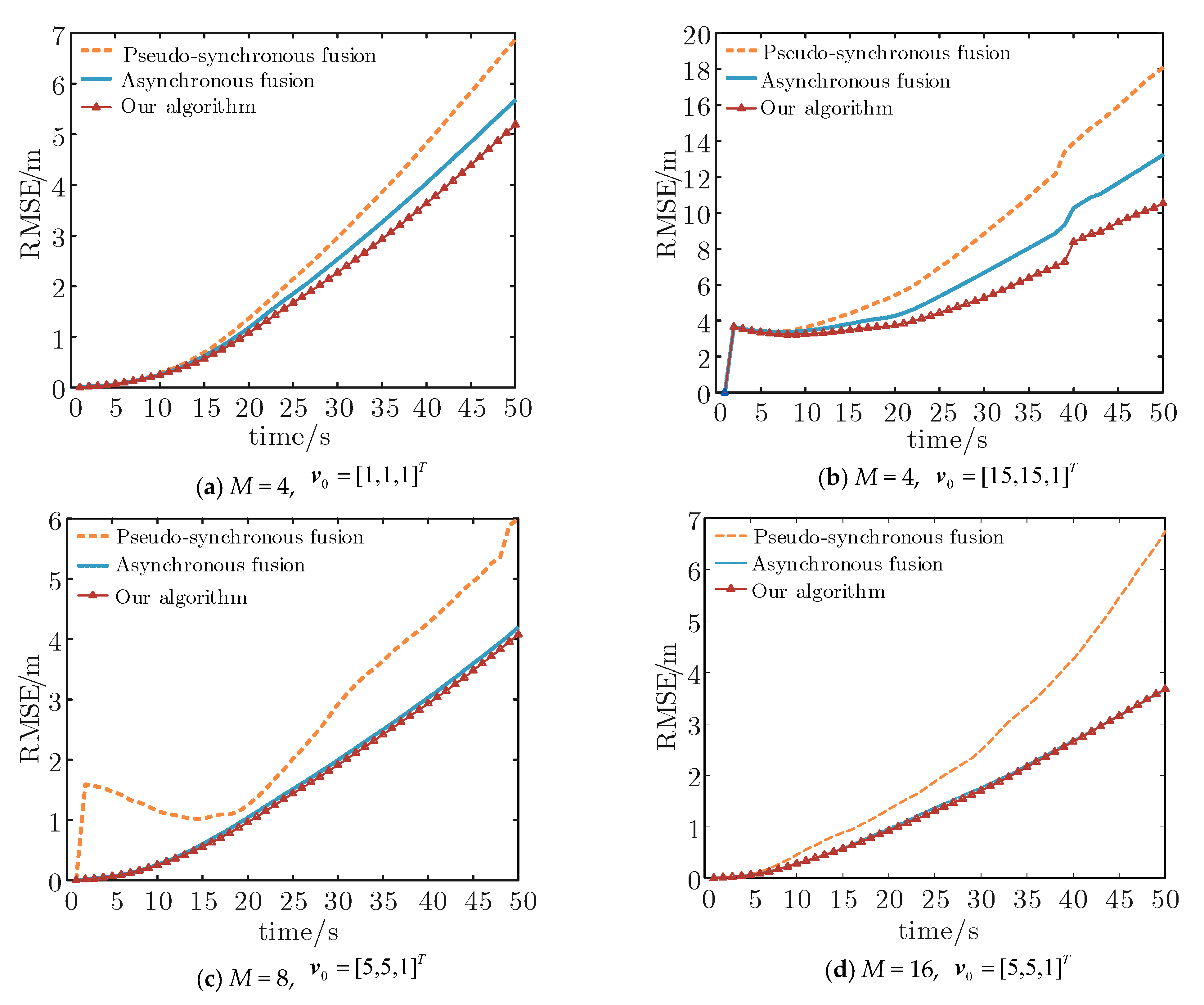
5. Simulation and Analysis

In this section, the proposed algorithm will be simulated and analyzed. The space of the tracking area is $500\mathrm{m}\times 500\mathrm{m}\times 500\mathrm{m}$. The underwater sensor network is composed of four nodes whose positions are (100 m, 300 m, 400 m), (50 m, 200 m, 20 m), (200 m, 50 m, 150 m) and (400 m, 400 m, 160 m). These four nodes are assumed to be homogeneous and can detect the target without bias. The variance of multiplicative noise ${\sigma }_{\delta }^2$ is 5 and the variance of additive noise ${\sigma }_v^2$ is $1.5\times {10}^{-4}$. The variance of process noise ${\omega }_{k-1}$ is $1\times {10}^{-4}{I}_{6\times 6}$. The initial state of the target ${\mathit{X}}_0=$ [100,5,100,5,100,1]^T; the initial estimate state of the target ${\widehat{\mathit{X}}}_0={\mathit{X}}_0$; the sampling interval is $T=1s$; the tracking lasts 50 s. The update factor is $\overline{a}=0.017$; the speed of sound is $\overline{b}=1473$. The number of particles in the particle filter is 1000. The simulation runs $MC=100$ times.

To indicate the accuracy of target tracking after node depth adjustment, root mean square error (RMSE) is adopted to measure the tracking performance, which is defined as:

$$\begin{array}{c}RMSE\left(k\right)=\sqrt{\frac{{\displaystyle \sum _{i=1}^{MC}{\left({\mathit{X}}_{\mathit{k}}-{\widehat{\mathit{X}}}_{\mathit{k}}\right)}^2}}{MC}}\end{array}$$

(33)

where $X_k$ and ${\widehat{X}}_k$ represent the real position and the estimated position of the target at time k, respectively.

In this study, simulations were carried out to verify that the effect of particle filter improved. Besides the proposed algorithm, the pseudo-synchronous fusion algorithm using the traditional PF [35] and the asynchronous fusion algorithm based on delay estimation [30] are also compared. The pseudo-synchronous fusion algorithm ignores the problem of transmission delay and regards the received measurements as synchronous data for fusion. The asynchronous fusion algorithm based on delay estimation takes the problem of inconsistency in propagation delay into consideration. However, it does not consider the ray tracing theory. Figure 4 shows the RMSE of each fusion algorithm.

It can be seen from Figure 4 that compared with pseudo-synchronous fusion, the proposed algorithm has better tracking effects, and it has further improved the asynchronous fusion based on delay estimation. In order to further verify the advantages of the proposed algorithm, simulations with different target initial speeds and node numbers are also carried out. The initial speeds of the target are ${\mathit{v}}_0=$ [5,5,1]^T ${\mathit{v}}_0=$ [1,1,1]^T ${\mathit{v}}_0=$ [15,15,1]^T respectively, and the number of nodes $M=4,8,16$. Figure 5 and

Table 1. Average RMSE of each fusion algorithm in various scenarios.

Number of Nodes	Target Speed	Algorithm in [35]	Algorithm in [30]	Our Algorithm
4	1,1,1	2.7358	2.1998	1.9915
4	5,5,1	4.7154	2.9405	2.6358
4	15,15,1	8.4613	6.5201	4.4348
8	5,5,1	2.6527	1.7071	1.6421
16	5,5,1	2.4136	1.5231	1.5008

present the comparisons of RMSE in various scenarios.

According to Figure 4 and Figure 5a,b, as the speed of the target increases, the RMSE of each algorithm increases as well. However, each algorithm is different in terms of its effectiveness at overcoming the impact of speed. Since the transmission delay is related to the speed of the target, the pseudo-synchronous fusion has the least effect on overcoming the impact of speed. Compared with the asynchronous fusion algorithm based on delay estimation, the proposed algorithm can overcome the tracking error more easily, as it considers the theory of ray tracing.

According to Figure 4 and Figure 5c,d, with the increase in the number of nodes, each algorithm can achieve better tracking accuracy. This is because more nodes can provide more measurements for fusion. However, compared with the four-node scenario, the improvement that occurs as a result of more nodes participating in tracking is limited, as seen in Figure 5c,d. Considering the limited energy of the underwater sensor network, too many nodes participating in tracking will consume a lot of energy. Therefore, from the perspective of balancing tracking accuracy and energy consumption, sparse USNs can achieve the best tracking performance. This also verifies the rationality of using four nodes for depth adjustment in our simulation.

Next, we simulate a case in which the target depth is known. In order to evaluate the effect of the proposed algorithm, the underwater target tracking based on a fixed node [11] is also simulated. Figure 6 shows the tracking effect under these two schemes. The detailed corresponding average RMSE and the average moving distance of nodes are shown in

Table 2. Average RMSE and the average moving distance of nodes where the target depth is known.

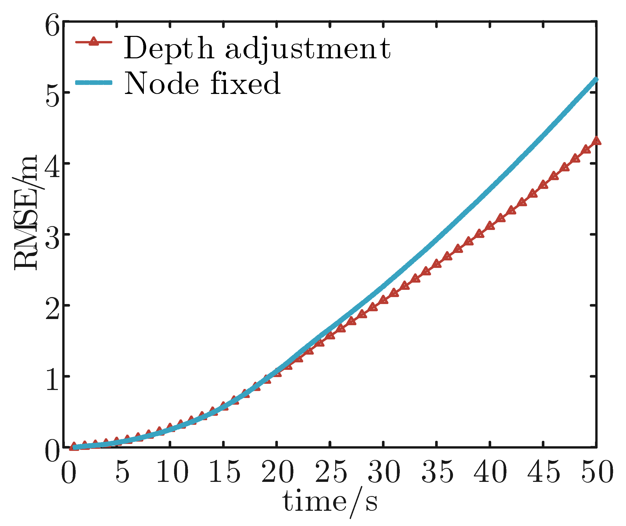
	Average RMSE/m	Average Moving Distance/m
Depth adjustment	1.7495	40
Node fixed	2.2898	0

. The tracking error improved by 23.59% following the depth adjustment. To a certain extent, this proves that there is an inevitable relationship between node depth adjustment and target tracking accuracy. By improving the node topology, the proposed depth adjustment algorithm has an obvious effect.

Considering that the maximum value of the node’s moving distance determines the extreme value of the height difference between the node and the target, the value of Dmax will affect the performance of the tracking algorithm based on depth adjustment. Figure 7 presents the tracking performance under different Dmax and

Table 3. Average RMSE and average moving distance of nodes where the target depth is known.

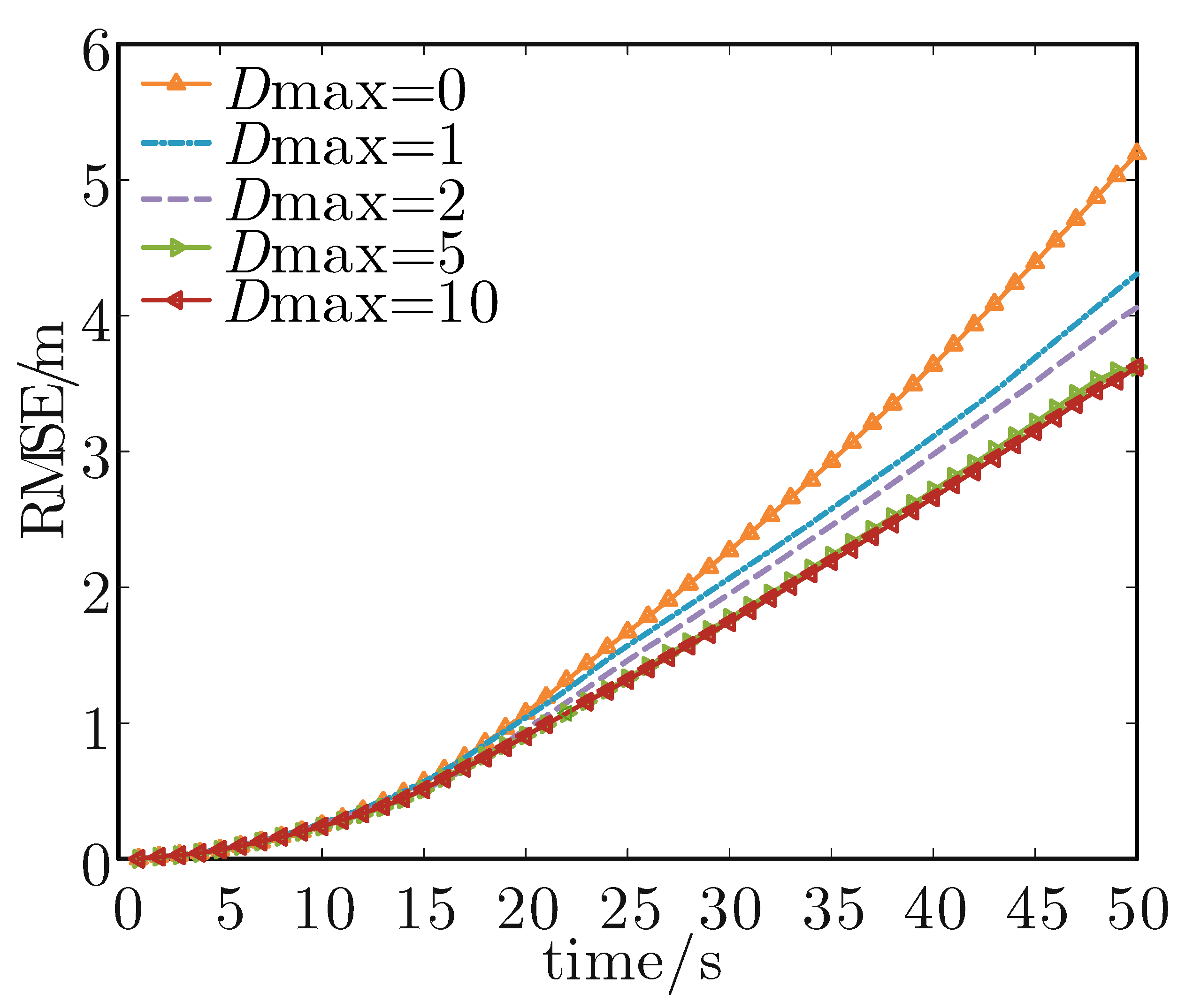
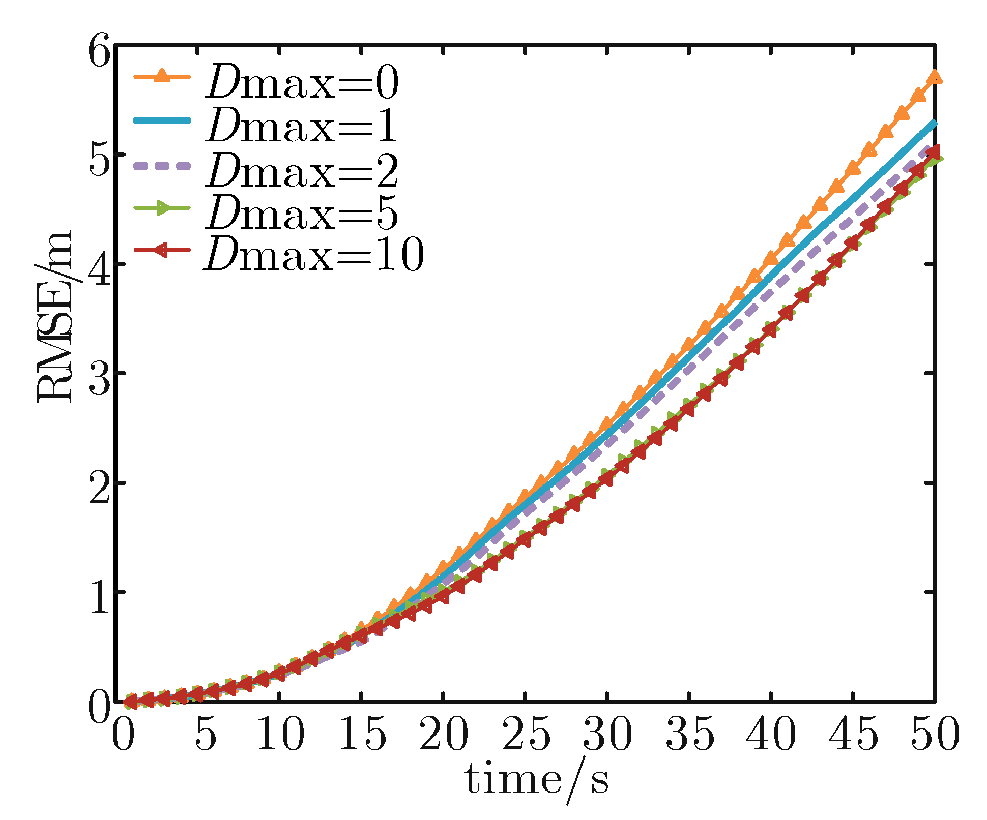
Dmax	Average RMSE/m	Average Moving Distance/m
0	2.2898	0
1	1.7495	40
2	1.6546	76.73
5	1.5175	169.49
10	1.4933	188.83

gives the detailed average RMSE and moving distance. It can be found from Figure 7 that the tracking error decreases with the increase in Dmax. This is because the larger the Dmax, the faster the mobile node reaches the topology with the maximum FIM.

Figure 8 further shows the depth variation of nodes under different Dmax. It can be seen from Figure 8 that the depth variation presents a linear relationship because the adjustment scheme given in (31) makes each node move in the direction where the height difference is at its maximum. At the same time, the target moves in constant velocity, so the moving distance of nodes varies linearly, as shown in Figure 8. As Dmax increases, the inflection point appears earlier. This also shows that underwater sensor nodes can reach the optimal depth position faster, providing more reliable and accurate measurements for target tracking. Combining Figure 8 and Table 3, it can be found that the tracking error and the average moving distance are a pair of contradictory quantities, and how to balance the relationship between them is a very important topic.

The effect of multiplicative noise on depth adjustment cannot be ignored. We make a comparison between the tracking performance of depth adjustment and node fixation under different multiplicative noises in Figure 9, and the detailed average RMSE and improvement under different multiplicative noises is shown in

Table 4. Average RMSE and improvement under different multiplicative noises where the target depth is known.

Multiplicative Noise	Algorithm	Average RMSE/m	Improvement
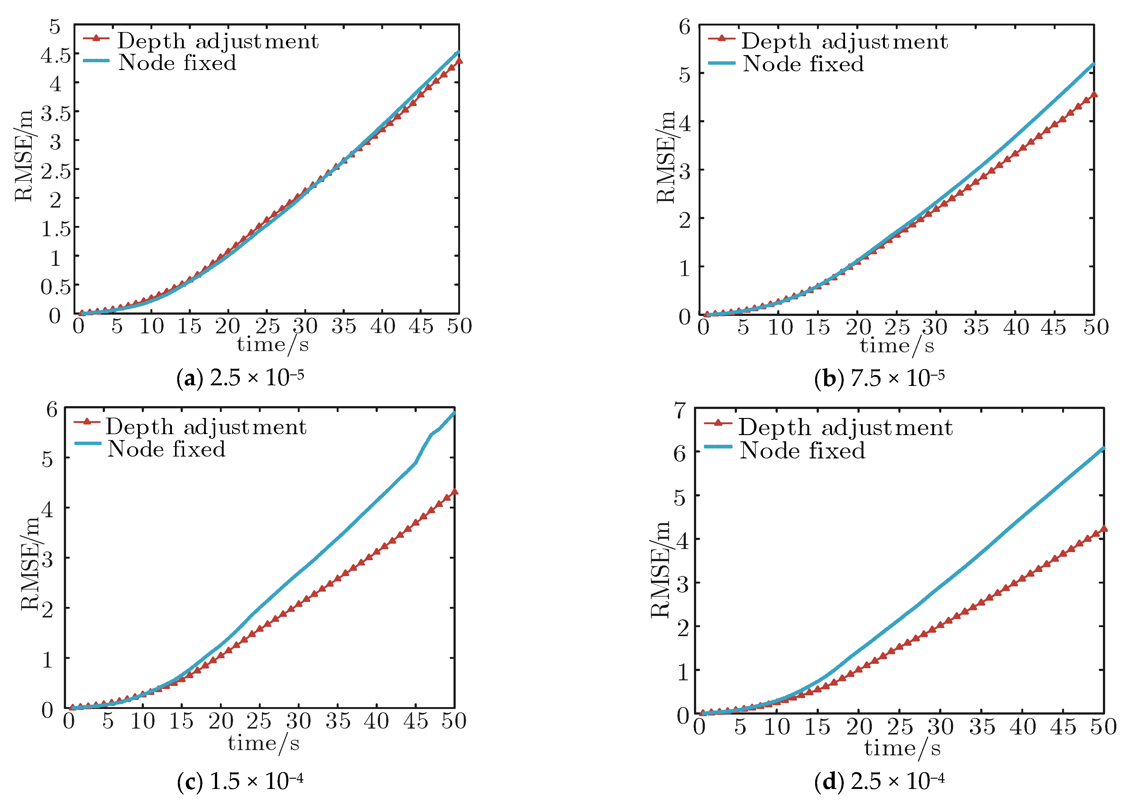
2.5 × 10−5	Depth adjustment	1.7866	0.30%
	Node fixed	1.7902
7.5 × 10−5	Depth adjustment	1.8494	9.35%
	Node fixed	2.0223
1.5 × 10−4	Depth adjustment	1.7495	30.89%
	Node fixed	2.2898
2.5 × 10−4	Depth adjustment	1.7148	43.81%
	Node fixed	2.4657

. From Figure 9, it can be determined that the RMSE of the depth adjustment algorithm does not decrease significantly with the increase in the multiplicative noise variance, because it will also be used as a part of the height adjustment objective function in the algorithm design process, and the same is true of height adjustment. Moreover, as the variance of multiplicative noise increases, the proposed algorithm improves the tracking performance more significantly than the algorithm with fixed nodes, which shows that the proposed algorithm is more suitable for measurement environments with severe multiplicative noise interference, especially in an underwater environment.

For a case in which the target depth is unknown, simulations are also carried out. Figure 10 presents the tracking performance of our algorithm under different Dmax, and

Table 5. Average RMSE and the average moving distance of nodes where the target depth is unknown.

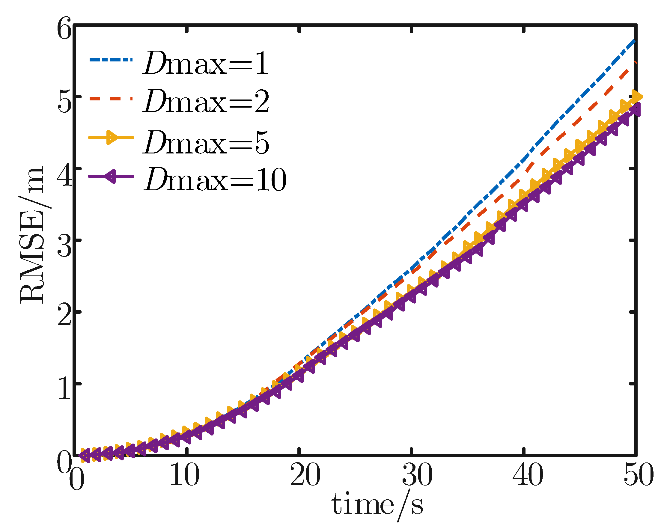
Dmax/m	Average RMSE/m	Average Moving Distance/m
0	2.2101	0
1	2.1061	41.09
2	2.0211	53.29
5	1.8759	137.49
10	1.8632	232.11

shows the average RMSE and moving distance of different Dmax. It can be seen from Figure 10 that the node depth adjustment algorithm after convex optimization can also improve the tracking accuracy. In this case, Dmax = 10 improves the tracking accuracy by 18.61% compared to when the node is fixed.

In addition to the node fixed scenario, the depth adjustment algorithm based on harmony search (HS) proposed in [23] is also simulated for comparison. Figure 11 and

Table 6. Average RMSE and the average moving distance of nodes achieved by HS when the target depth is unknown.

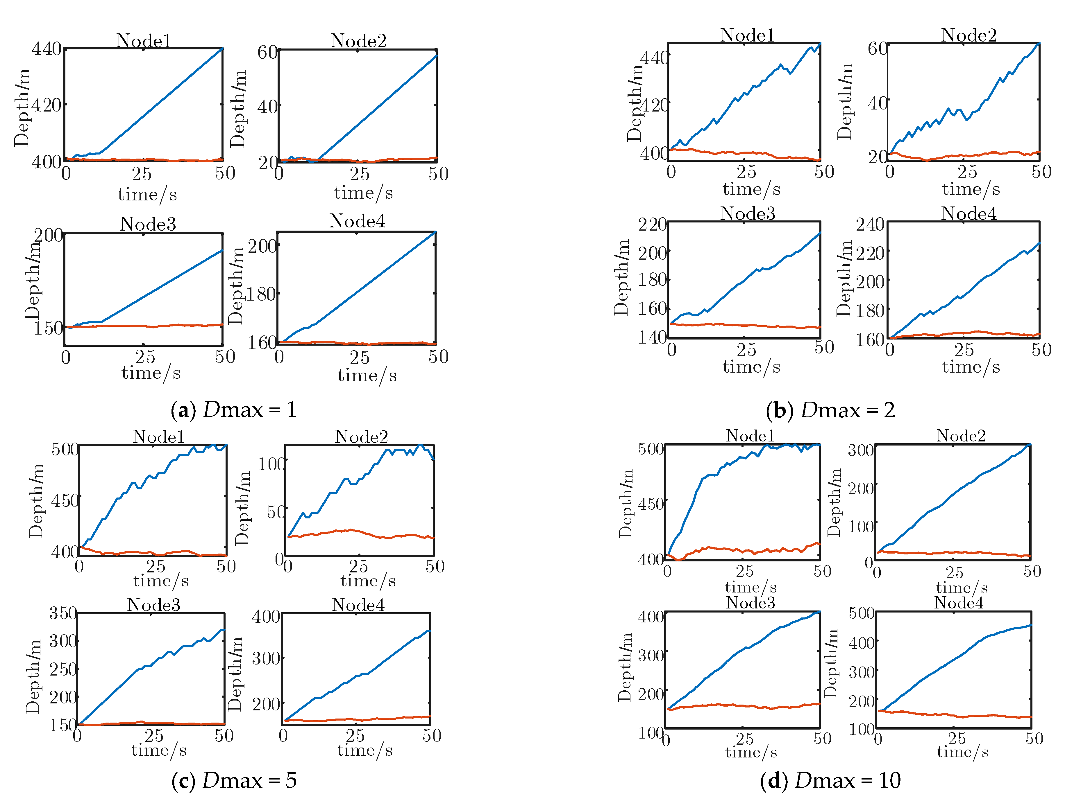
Dmax/m	Average RMSE/m	Average Moving Distance/m
1	2.2741	0.31
2	2.1781	2.38
5	1.9976	5.15
10	1.9224	13.35

show the results obtained by HS. It can be found that the node depth adjustment algorithm based on HS can also improve the tracking accuracy. However, since the HS is an intelligent optimization algorithm, the result obtained is not unique, and the optimization result is unstable. Compared with the depth adjustment algorithm based on convex optimization, the tracking effect is worse.

The average moving distance of all nodes under different Dmax are further presented in Figure 12. Obviously, the node depth adjustment presents a nonlinear relationship because the target depth is unknown in this case. The four nodes have different depth adjustment processes, which can adjust the position more flexibly and build a more complete topology.

Since the time complexity of the algorithm is calculated in this paper, we also design the corresponding simulation for verification in this part. Figure 13 presents the running time of the two algorithms under different Dmax. It can be seen from Figure 13 that the interior point algorithm can reach convergence faster and achieve deep adjustment.

The above simulations show that when the target depth is unknown, the depth adjustment algorithm based on the interior point method has excellent results. When using the same number of underwater sensor nodes to participate in target tracking, the depth adjustment algorithm based on the interior point method can not only obtain the optimal depth adjustment strategy with a faster convergence speed than the intelligent optimization algorithm, but can also adaptively adjust the node topology, obtain more complete measurement data and effectively improve tracking accuracy.

6. Conclusions

This paper proposes a node depth adjustment algorithm for target tracking in sparse USNs. Node depth adjustment is described as an optimization problem of maximizing the value of Fisher information matrix. Two different convex optimization methods are used to adjust node depth when the target depth is known and unknown. Compared to other algorithms, the algorithm proposed in this paper considers the acoustic transmission delay and node topology. The simulations illustrate that the proposed algorithm is superior and more robust to the comparison algorithm in tracking accuracy; a better node topology can be obtained, and the measurement data can be improved with the help of node depth adjustment. Future work will further improve the algorithm combination with node energy consumption. For example, considering the two different types of indicators of node energy consumption and tracking accuracy, a multi-objective depth adjustment problem is constructed to achieve energy efficiency optimization in the process of underwater target tracking. We will also combine machine learning technology to design a depth adjustment algorithm that is more suitable for dense underwater sensor networks.

References

- Luo, J.; Han, Y.; Fan, L. Underwater acoustic target tracking: A review. Sensors 2018, 18, 112. [Google Scholar] [CrossRef] [PubMed]
- Ghafoor, H.; Noh, Y. An overview of next-generation underwater target detection and tracking: An integrated underwater architecture. IEEE Access 2019, 7, 98841–98853. [Google Scholar] [CrossRef]
- Su, X.; Ullah, I.; Liu, X.; Choi, D. A review of underwater localization techniques, algorithms, and challenges. J. Sens. 2020, 2020, 6403161. [Google Scholar] [CrossRef]
- Liu, M.; Han, X.; Zhang, S.; Zheng, R.; Lan, J. Research status and prospect of target tracking technologies via underwater sensor networks. Acta Autom. Sin. 2021, 47, 235–251. [Google Scholar] [CrossRef]
- Zhang, Y.; Gao, L. Target Tracking with Underwater Sensor Networks Based on Grubbs Criterion and Improved Particle Filter Algorithm. J. Electron. Inf. Technol. 2019, 41, 2294–2301. [Google Scholar] [CrossRef]
- Ullah, I.; Chen, J.; Su, X.; Esposito, C.; Choi, C. Localization and detection of targets in underwater wireless sensor using distance and angle based algorithms. IEEE Access 2019, 7, 45693–45704. [Google Scholar] [CrossRef]
- Wang, W.; Li, X.; Zhang, K.; Shi, J.; Shi, W.; Ali, W. Robust Direction Finding via Acoustic Vector Sensor Array with Axial Deviation under Non-Uniform Noise. J. Mar. Sci. Eng. 2022, 10, 1196. [Google Scholar] [CrossRef]
- Hwang, J.; Bose, N.; Nguyen, H.D.; Williams, G. Acoustic search and detection of oil plumes using an autonomous underwater vehicle. J. Mar. Sci. Eng. 2020, 8, 618. [Google Scholar] [CrossRef]
- Liu, H.; Xu, B.; Liu, B. A Tracking Algorithm for Sparse and Dynamic Underwater Sensor Networks. J. Mar. Sci. Eng. 2022, 10, 337. [Google Scholar] [CrossRef]
- Yan, J.; Zhao, H.; Pu, B.; Luo, X.; Chen, C.; Guan, X. Energy-efficient target tracking with UASNs: A consensus-based Bayesian approach. IEEE Trans. Autom. Sci. Eng. 2019, 17, 1361–1375. [Google Scholar] [CrossRef]
- Zhang, D.; Liu, M.-Q.; Zhang, S.-L.; Fan, Z.; Zhang, Q.-F. Mutual-information based weighted fusion for target tracking in underwater wireless sensor networks. Front. Inf. Technol. Electron. Eng. 2018, 19, 544–556. [Google Scholar] [CrossRef]
- Tian, S.; Zhang, Z. A Node Selection Algorithm Based on Multi-objective Optimization under Position Floating. IEEE Access 2022, 10, 1. [Google Scholar] [CrossRef]
- Zhang, S.; Chen, H.; Liu, M.; Zhang, Q. Optimal quantization scheme for data-efficient target tracking via UWSNs using quantized measurements. Sensors 2017, 17, 2565. [Google Scholar] [CrossRef]
- Zhang, Q.; Liu, M.; Zhang, S. Node topology effect on target tracking based on UWSNs using quantized measurements. IEEE Trans. Cybern. 2014, 45, 2323–2335. [Google Scholar] [CrossRef]
- Xu, S.; Doğançay, K. Optimal sensor placement for 3-D angle-of-arrival target localization. IEEE Trans. Aerosp. Electron. Syst. 2017, 53, 1196–1211. [Google Scholar] [CrossRef]
- Song, Y. Underwater acoustic sensor networks with cost efficiency for internet of underwater things. IEEE Trans. Ind. Electron. 2020, 68, 1707–1716. [Google Scholar] [CrossRef]
- Li, B.; Chen, C. Fish-action hunt policy for underwater sensor deployment. J. Nanjing Univ. Sci. Technol. 2019, 43, 244–249. [Google Scholar] [CrossRef]
- Latif, K.; Javaid, N.; Ullah, I.; Kaleem, Z.; Abbas Malik, Z.; Nguyen, L.D. DIEER: Delay-intolerant energy-efficient routing with sink mobility in underwater wireless sensor networks. Sensors 2020, 20, 3467. [Google Scholar] [CrossRef]
- Banaeizadeh, F.; Toroghi Haghighat, A. An energy-efficient data gathering scheme in underwater wireless sensor networks using a mobile sink. Int. J. Inf. Technol. 2020, 12, 513–522. [Google Scholar] [CrossRef]
- Jiang, P.; Liu, S.; Liu, J.; Wu, F.; Zhang, L. A depth-adjustment deployment algorithm based on two-dimensional convex hull and spanning tree for underwater wireless sensor networks. Sensors 2016, 16, 1087. [Google Scholar] [CrossRef]
- Yang, Z.; Shi, X.; Chen, J. Optimal coordination of mobile sensors for target tracking under additive and multiplicative noises. IEEE Trans. Ind. Electron. 2013, 61, 3459–3468. [Google Scholar] [CrossRef]
- Tian, S.; Zhang, Z. Tracking Energy Control Algorithm Based on Underwater Sensor Networks Assisted by AUV. In Proceedings of the International Conference on Autonomous Unmanned Systems, Changsha, China, 24–26 September 2021; Springer: Singapore, 2021; pp. 379–388. [Google Scholar] [CrossRef]
- Liu, M.; Zhang, D.; Zhang, S.; Zhang, Q. Node depth adjustment based target tracking in UWSNs using improved harmony search. Sensors 2017, 17, 2807. [Google Scholar] [CrossRef] [PubMed]
- Luo, J.; Han, Y. A node depth adjustment method with computation-efficiency based on performance bound for range-only target tracking in UWSNs. Signal Process. 2019, 158, 79–90. [Google Scholar] [CrossRef]
- Zhao, Y.; Li, Z.; Hao, B.; Shi, J. Sensor selection for TDOA-based localization in wireless sensor networks with non-line-of-sight condition. IEEE Trans. Veh. Technol. 2019, 68, 9935–9950. [Google Scholar] [CrossRef]
- Yan, Q.; Chen, J. Sensor Selection Method Based on Multi-objective Optimal Optimization for Mixture Gaussian Noise. J. Electron. Inf. Technol. 2021, 43, 341–348. [Google Scholar] [CrossRef]
- Liu, B.; Tangy, X.; Tharmarasa, R.; Kirubarajan, T.; Jassemi, R.; Halle, S. Underwater target tracking in uncertain multipath ocean environments. IEEE Trans. Aerosp. Electron. Syst. 2020, 56, 4899–4915. [Google Scholar] [CrossRef]
- Bass, A.H.; Clark, C.W. The Physical Acoustics of Underwater Sound Communication. In Acoustic Communication; Springer: New York, NY, USA, 2003; pp. 15–64. [Google Scholar]
- Zhu, G.; Zhou, F.; Xie, L.; Jiang, R.; Chen, Y. Sequential asynchronous filters for target tracking in wireless sensor networks. IEEE Sens. J. 2014, 14, 3174–3182. [Google Scholar] [CrossRef]
- Liu, M.; Zhao, L.; Zhang, S. Delay-estimation-based asynchronous particle filtering for passive target tracking in underwater wireless sensor networks. In Proceedings of the 2017 36th Chinese Control Conference (CCC), Dalian, China, 26–28 July 2017; pp. 8929–8934. [Google Scholar] [CrossRef]
- Brekhovskikh, L.M.; Lysanov, Y.P.; Lysanov, J.P. Fundamentals of Ocean Acoustics; Springer Science & Business Media: Berlin, Germany, 2003. [Google Scholar]
- Zhao, H.; Yan, J.; Luo, X.; Guan, X. Ubiquitous Tracking for Autonomous Underwater Vehicle with IoUT: A Rigid-Graph-Based Solution. IEEE Internet Things J. 2021, 8, 14094–14109. [Google Scholar] [CrossRef]
- Isbitiren, G.; Akan, O.B. Three-dimensional underwater target tracking with acoustic sensor networks. IEEE Trans. Veh. Technol. 2011, 60, 3897–3906. [Google Scholar] [CrossRef]
- Zhang, J.; Wu, C.; Zhang, Y.; Ji, P. Energy-efficient adaptive dynamic sensor scheduling for target monitoring in wireless sensor networks. ETRI J. 2011, 33, 857–863. [Google Scholar] [CrossRef]
- Pozna, C.; Precup, R.-E.; Horvath, E.; Petriu, E.M. Hybrid Particle Filter–Particle Swarm Optimization Algorithm and Application to Fuzzy Controlled Servo Systems. IEEE Trans. Fuzzy Syst. 2022, 30, 4286–4297. [Google Scholar] [CrossRef]
- Greco, C.; Vasile, M. Robust Bayesian particle filter for space object tracking under severe uncertainty. J. Guid. Control. Dyn. 2022, 45, 481–498. [Google Scholar] [CrossRef]
- Cao, N.; Choi, S.; Masazade, E.; Varshney, P.K. Sensor selection for target tracking in wireless sensor networks with uncertainty. IEEE Trans. Signal Process. 2016, 64, 5191–5204. [Google Scholar] [CrossRef]
- Masazade, E.; Niu, R.; Varshney, P.K. Dynamic bit allocation for object tracking in wireless sensor networks. IEEE Trans. Signal Process. 2012, 60, 5048–5063. [Google Scholar] [CrossRef]
- Sun, J.; Shi, G. Cost-efficient node deployment for intrusion detection in underwater sensor networks. In Proceedings of the 2019 IEEE 25th International Conference on Parallel and Distributed Systems (ICPADS), Tianjin, China, 4–6 December 2019; pp. 633–638. [Google Scholar] [CrossRef]
- Moreno-Salinas, D.; Pascoal, A.; Aranda, J. Sensor networks for optimal target localization with bearings-only measurements in constrained three-dimensional scenarios. Sensors 2013, 13, 10386–10417. [Google Scholar] [CrossRef]
- Zhang, Q.; Liu, M.; Zhang, S.; Chen, H. Node topology effect on target tracking based on underwater wireless sensor networks. In Proceedings of the 17th International Conference on Information Fusion (FUSION), Salamanca, Spain, 7–10 July 2014; pp. 1–8. [Google Scholar]
- Chen, S. The KKT optimality conditions for optimization problem with interval-valued objective function on Hadamard manifolds. Optimization 2022, 71, 613–632. [Google Scholar] [CrossRef]
- Boyd, S.; Boyd, S.P.; Vandenberghe, L. Convex Optimization. Cambridge University Press: Cambridge, UK, 2004. [Google Scholar]