Abstract
This paper investigates a fault-tolerant control problem for the dynamic positioning of unmanned marine vehicles based on a Takagi–Sugeno (T-S) fuzzy model using an integral sliding mode scheme. First, the T-S fuzzy model of an unmanned marine vehicle is established by taking the yaw angle variable range into account. An integral sliding mode control scheme combined with the performance index is then developed to attenuate the initial influence of thruster faults and ocean disturbances. The unknown nonlinear function is approximated using a fuzzy logic system based on a representation of marine data, which provides a good tradeoff between resolution of the unknown nonlinear term approximation and computational complexity for marine engineering by adjusting the number of fuzzy logic system rules. In addition, the fault estimation information is utilized to design the sliding mode surface on the basis of an adaptive mechanism and a matrix full rank decomposition technique, which reduces conservatism. The validity of the proposed approach is finally demonstrated by an analysis of simulation results using a typical floating production vessel model.
1. Introduction
As an important offshore operating platform in recent decades, unmanned marine vehicles (UMV) have a wide range of applications including scientific exploration, mineral resources sampling, environmental monitoring, military reconnaissance, and more [1,2,3,4,5,6,7]. These applications have contributed to the development of UMV motion control in theory and implementation, and significant advances have been achieved, including heading control [8], trajectory tracking control [9], formation control [10], and others. In addition to the aforementioned topics, the dynamic positioning (DP) problem for UMV has attracted the attention of many scholars [11,12,13,14,15]. In [11], the authors designed a DP controller by taking advantage of and mixed- techniques to improve the robustness of the DP system. A dynamic surface control approach was proposed in [12] for ship dynamic positioning systems (DPS) to eliminate the impact of input saturation and unknown time-varying disturbances in the meantime. In [13], a synchronous online optimal control was developed for DPS to avoid repetitive computation and save runtime while guaranteeing the real-time performance of the control scheme. A model predictive control technique on the base of state-space equations was used for a ship DPS in [14]. Again for DPS, an adaptive discrete-time optimal control strategy was investigated in [15] based on adaptive dynamic programming and a broad learning system to save energy and time.
Admittedly, the above literature shows that good results have been achieved in the UMV DP problem. As stated in [16], modeling resolution can be improved by increasing the number of the fuzzy local models. However, the corresponding computational complexity increases as well, making control synthesis and stability analysis more difficult. Fortunately, the T-S fuzzy model is a very useful tool to express this kind of complex nonlinear system with uncertainties. The primary characteristic of a T-S fuzzy model is the use of a linear system model to represent the local dynamics of each fuzzy rule, which provides the breadth and convenience of using mature linear theory to solve nonlinear control problems [17]. Thus, the T-S fuzzy model has quickly become a hot spot in the field of DP research; for example, quadratic finite-horizon optimal control problems have been solved using a hybrid Taguchi-genetic algorithm and orthogonal function approach for T-S fuzzy control of DPS in [18]. In [19], a robust DP controller was developed by utilizing an optimal control strategy and a T-S fuzzy method. Network-based modeling, controller design, and stability analysis for observer-based T-S fuzzy DPS were investigated in [20]. Although the T-S fuzzy models in the above-mentioned literature achieved good results, they simplified the original nonlinear system as far as possible, resulting in loss of modeling resolution. On the other hand, for T-S fuzzy models, when the resolution is increased by increasing the number of the fuzzy local models, the complexity is increased as well, which makes control synthesis and stability analysis more difficult. Therefore, the first aim of this paper is to achieve a good tradeoff between modeling resolution and computational complexity in T-S models for UMVs.
In another research scenario, the failure of UMV propellers is inevitable in the complex marine environment; the failure of a propeller may cause performance loss or mission abort, and can even cause serious consequences for navigational safety [21,22,23]. Therefore, it is essential to study fault-tolerant control (FTC) of UMV [24,25,26,27,28]. At present, progress is being made in this field. For example, an FTC method based on fault detection and identification (FDI) was proposed in [24] to improve ship operational reliability. A control allocation algorithm based on the estimates of isolated and identified actuator failures was utilized to carry out fault-tolerant control allocation in [25]. It should be noted that the aforementioned controllers were designed by obtaining all or part of the propeller failure information in advance. However, in a complex marine environment the FDI may cause false alarms or undetected faults, which can have a negative impact on FTC. To avoid this situation, developing robust fault-tolerant controllers independent of the FDI is wise. In [26], a quantized sliding mode fault-tolerant controller without an FDI module was designed to solve the quantization-based DP control problem for a UMV. A novel robust adaptive fault-tolerant control scheme for the path-following problem of UMVs was provided in [27]. A novel quantized sliding mode FTC design scheme for UMV under a T-S fuzzy model framework was provided in [28] to compensate for the effects of thruster faults. However, the sliding mode control design schemes in the above studies cannot ensure that the system always meets the desired robustness from the initial stage, which means that the system is sensitive to perturbations satisfying the matching condition, as it has not yet reached the sliding manifold in the initial period of time. In other words, after the system begins to maintain the sliding manifold at the very beginning, it has the advantage of being robust throughout the entire system response phase against thruster faults, which can be modeled as matched uncertainty. Thus, another motivation of ours is to design a fault-tolerant controller that can guarantee robustness from the initial stage of the T-S fuzzy model for UMVs with thruster failures.
Inspired by the above discussion, the DP problem for T-S fuzzy models in UMVs with actuator faults is addressed in this paper. An integral sliding mode control (ISMC) scheme considering the fault estimation information is developed to ensure that the T-S fuzzy UMV model is robust from the initial stage.
The main contributions of this article are as follows:
- (1)
- Using a T-S fuzzy model with an adjustable number of fuzzy logic system (FLS) to locally approximate the nonlinear terms of a UMV model in order to achieve a good compromise between modeling resolution and computational complexity.
- (2)
- An ISMC methodology with fault information is applied to design the fault-tolerant controller for the T-S fuzzy UMV model such that the conservatism of the controller can be reduced and the robustness and fault-tolerance of the UMV controller are guaranteed from the initial time.
The rest of this article is structured as follows: Section 2 presents the system description and preliminary knowledge; in Section 3, the main results of the ISMC scheme are provided; a simulation case study is provided to illustrate the merit of the proposed method in Section 4; finally, our conclusions are presented in Section 5.
Notation: for matrix Y, the symbols , , and express the inverse, pseudo-inverse, and transpose of matrix Y, respectively. Positive definite and semi-positive-definite matrices are denoted by the notations and . A diagonal matrix with the diagonal elements is written as . Here, “*” stands for a term produced by matrix symmetry. The notations O and I express the zero and identity matrices, respectively. means a Euclidean space with n-dimensions. The symbol is utilized to express the Euclidean norm of the vector p. Finally, the exponential function with base e is expressed by the symbol .
2. Problem Formulation
2.1. Umv Model
For a UMV operating in surge, sway, and yaw, the equation of motion is
where means the velocity vector of the UMV described in the body-fixed frame, as shown in Figure 1, which consists of the surge velocity , the sway velocity , and the yaw velocity . Moreover, is the earth-fixed orientation vector formed with positions , , and the heading angle . expresses the unified thruster fault model, described as follows [26]:
where is an unknown actuator effectiveness level matrix, and is a diagonal weighting matrix with and , for and , l, j, m, and n express the lth thruster, the jth malfunction mode, the total number of thrusters, and the number of fault modes respectively. Here, or ; the stuck fault is bounded by , which can be shown in Table 1. Moreover, , represents ocean disturbances, the form of which can be seen in [20]; finally, M, N, and G express the matrix of inertia, the matrix of damping, and the matrix of mooring forces, respectively. For an arbitrary angle , the thruster configuration matrix E [29] can be defined as
where expresses the moment arms with and
with
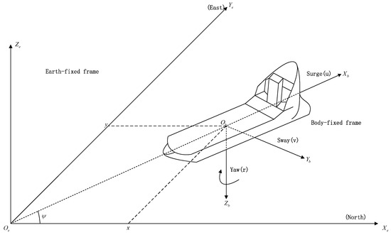
Figure 1.
UMV in the reference coordinate system.

Table 1.
Table of fault types.
Because represents a nonlinear function of , let [2,26]. Then, the following equation can be derived from (1):
where , , , and .
2.2. T-S Fuzzy UMV Modeling
Establishing T-S fuzzy models for the UMV is the goal of this subsection. The system below is derived by letting and combining (3) with (4):
It is reasonable to consider that the variation scope of the yaw angle ranges from to [20]. Furthermore, we can derive that , . Then, the T-S fuzzy UMV system is obtained by adopting the rules below.
where ; and are fuzzy sets and is the regulated output:
, , , , , , , , where is a known matrix. For convenience, is abbreviated to .
Then the global T-S fuzzy UMV model of (6) is described as
where .
Remark 1.
It should be mentioned that there exist the nonlinear terms and in system (5), which are modeled by constructing the T-S fuzzy models.
Before the fault-tolerant controller is designed, we assume the following.
Assumption 1.
For all unknown actuator effectiveness levels , , all pairs are completely controllable.
Assumption 2.
All actuators could have loss-of-effectiveness failures at the same time; nevertheless, the remaining actuators have the capability of completing the intended control task even while up to actuators become stuck or experience an outage.
Assumption 3.
There exist unknown constants and which make the nonparametric actuator stuck fault and external disturbances piecewise continuous with as the bound.
Assumption 4.
for all , .
Remark 2.
The first two assumptions above ensure that the FTC system is internally stable and that the actuator failure accommodation problem has a feasible solution [26,28], respectively. Assumption 3 is natural and widely used [30]. The actuator redundancy condition in Assumption 4 accommodates stuck faults and outages [26,28].
The later control law design makes use of the following definition and two lemmas.
Definition 1
([31]). Let a closed-loop system be defined as
For any , if is valid, where , then it is said that the system (8) satisfies an adaptive performance index that is no more than .
Lemma 1
This article is aimed at constructing an appropriate integral sliding surface and an integral sliding mode (ISM) fault-tolerant controller for a T-S fuzzy model of a UMV that can guarantee system stability and achieve the performance index shown in Definition 1 in the presence of thruster failures and external disturbance. The whole control strategy is shown in Figure 2.
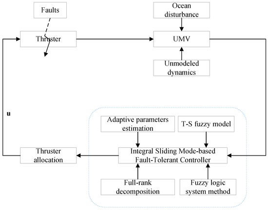
Figure 2.
Integral sliding mode fault-tolerant strategy for T-S model of UMV with faults.
3. Integral Sliding Mode Fault-Tolerant Compensation Strategy Design
This section introduces an integral sliding surface design approach by combining a matrix factorization method with an adaptive mechanism. Then, the existing conditions of the integral sliding surface design scheme are provided by a linear matrix inequality (LMI). Here, , , , and are the estimation parameters updated by the adaptive law, representing the unknown weighted matrix, the approximation error, the disturbance upper bounds, and the unknown fault information respectively. Furthermore, an ISM FTC law is developed to guarantee the stability of the sliding dynamics and subsequent sliding mode maintenance.
Suppose that has a matrix full-rank decomposition as follows:
where , , and [26].
Lemma 2
for every .
Then, an FLS is used to find an approximation of the unknown smooth function in (7). The ability to uniformly approximate any nonlinear smooth function defined on compact sets is well demonstrated in the literature [32]. Thus, it is not difficult to obtain the following equation by taking advantage of the properties of an FLS:
where denotes an unknown adjustable parameter vector, represents a fuzzy basis function vector (which is commonly selected as a Gaussian function to ensure that the basis vector is positive), M expresses the number of FLS rules, and is an unknown constant bound of the approximate error which satisfies
Remark 3.
The unknown nonlinear term is present in the T-S fuzzy UMV model (7), because the yaw angle of the DPS varies within a certain range. Though [28] used a linear matrix inequality to deal with it, only the sector bounds were used, which leads to conservativeness. To compensate for the effects of the nonlinear term more accurately, an FLS is utilized in this paper, which can exploit a good tradeoff between conservatism and computational burden by adjusting the number of FLS rules M.
The following two components make up the ISM controller developed in this paper:
where
where , and ; the term is the linear part, the function of which is to attenuate disturbances, while is the discontinuous control term of the controller, which is used to reject nonlinearity terms and force the system state onto the sliding manifold in (16). Let the parameter be the positive number introduced in Lemma 2. In particular, is an approximation of with and
where and denote the smallest eigenvalue of and any positive scalar, respectively, while , and represent estimates of the upper bound of the reconstruction error , the weight matrix , the fault impact factor , the stuck fault upper bound , and the disturbance upper bound , respectively.
The definition of the integral sliding manifold is provided by the set below:
and the integral switching surface in this paper is constructed using the following form:
where is a freely designed matrix that meets condition (19) and in (17) is the estimated matrix of , which can use the projection algorithms below to update
where , , , and are the adjusted parameter, the ith column of input matrix , and the ith row of gain matrix K in the jth fuzzy rule, respectively.
The reaching phase is avoided [33], as the term satisfies .
According to the literature [33],
Remark 4.
As far as the authors know, little fault information has been considered in the design of previous sliding surfaces for FTC using T-S fuzzy models (7). In this paper, estimation of the actuator efficiency factor is used in (17) to construct the sliding manifold for the T-S fuzzy mode of the UMV, which makes full use of the fault information to achieve better robustness and less conservatism than the traditional construction method.
The following Theorem 1 demonstrates the existing conditions of the sliding dynamics on the provided integral sliding surface (17), showing that the performance index cannot be greater than when there are external disturbances and actuator failures.
Theorem 1.
The sliding mode dynamics are asymptotically stable at the beginning and the performance index is not greater than if there exists and matrix that makes the following inequality hold for the integral sliding surface (17):
Proof.
The derivative of the integral sliding surface (17) can be obtained as follows:
Because , , we have . An equivalent control [34] is therefore achieved as follows:
Substituting (23) into (7) and taking advantage of the property that , the following equation is derived:
Using G as described in (19) and as specified in (14), subsequent simplification of Equation (24) yields
By Schur’s complement lemma and Lemma 1, if there exists matrix such that the inequality
holds, where , then the quadratic stability of the sliding dynamics and the performance index are assured.
Application of Schur’s complement lemma can be used to show that Equation (20) is equivalent to . Consequently, with , inequality (26) is true. As a result, the performance index is satisfied from the start, and the sliding dynamics are guaranteed to exist.
The proof is completed. □
Remark 5.
Remark 6.
Sliding-mode control can be maintained from the very beginning using the ISM technique [35,36,37,38]. Compared with the traditional sliding mode control strategy in [26], greater robustness against actuator faults can be obtained.
The matrix decomposed forms used in the subsequent analysis are defined as follows:
where and .
Before the main points are presented, the following adaptive laws are provided:
where is as shown in (15), and
, and are bounded initial values of , and , respectively. The design parameters , and are positive.
We define
Because , and are unknown constants, it is not difficult to obtain the error systems
Remark 7.
It can be seen from (27) that is true for with . Obviously, for the purposes of this paper we can further assume that . Therefore, can be obtained.
The reachability analysis of the ISM is provided by the following theorem.
Theorem 2.
Proof.
Let , then consider the candidate Lyapunov function below for the analysis of reachability:
where .
Deriving with respect to time by substituting the system (7), the outcome is
Recalling the property , the above inequality (32) can be reorganized into the following equation:
For convenience, we abbreviate as . It is proven that the inequalities below are true according to Assumption 2:
Considering (14), we can obtain
Further, the following property holds:
Obviously, is true for with in consideration of the adaptive mechanism (27). From Lemma 2, we can derive the inequality
where was introduced in (15). Now, it is easily obtained from (38) that
Moreover, based on the adaptive laws listed in (27), it is not difficult to show that . Therefore, the inequality can be obtained from (40), which means that is not an increasing function. Thus, the inequality is valid, that is, . It follows that exists, as . Then, the inequality below is obtained by integrating (40) on both sides simultaneously:
Further, as , can be obtained from the aforementioned inequality (41), which means that . Therefore, if the Barbalat lemma is applied to (8), the trajectories of the system stay on the integral sliding manifold defined in (16).
Thus, the proof is completed.
4. Simulation Result
This part shows the validity of the proposed methodology. Let the parameter matrices of the UMV model [19,20] be
, ,
, .
Figure 3 shows the position distribution of the thrusters.
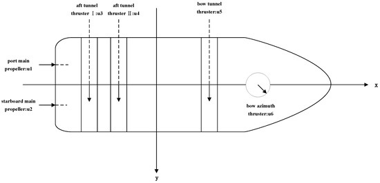
Figure 3.
Schematic drawing showing the UMV thruster configuration.
The ocean disturbances model is provided by [20]:
where the shaping filter is with dominant wave strength coefficient , damping coefficient , wave encounter frequency , and band-limited white noise with noise power is 2.69. Similarly, with , , , and with noise power 1.56. Moreover, let
The nonlinear term vector can be chosen as
Table 2.
Rule table of the T-S fuzzy model.
Additionally, in the simulation, after 30s we assume a loss of effectiveness 40% and stuck at on the bow tunnel thruster and the aft tunnel thruster I, respectively. The part in (14) is replaced by a continuous approximation to attenuate chattering.
For the simulation, and the initial state are chosen.
The following fuzzy membership functions can be defined:
Thus, the fuzzy basis functions can be expressed as
In this case, is chosen as .
The relation holds by validation. Moreover, the following initial estimation parameters and adjustment gain values are used:
.
The results of this article are compared with those that do not take the impact of thruster failures into account in [20] to demonstrate the validity of the proposed T-S fuzzy DP control methodology. The response curves from this paper are shown using red solid lines in Figure 4 and Figure 5, while the simulation results without taking thruster faults into account are shown using blue solid lines. Figure 4 depicts the state response of the proposed methodology. It can be clearly seen that the states in this article converge to zero in the end, whereas the comparison simulation shows a divergence from s. The control signals in Figure 5 indicate that the proposed controller works well, especially when thruster failures are present. In summary, the control approach in Section 3 offers much better control performance compared to the controller that does not take thruster failures into account. Adaptive parameter adjustments are shown in Figure 6, Figure 7, Figure 8 and Figure 9. It is easy to observe that they are convergent and meet our expectations. The ocean disturbance parameters were adjusted as follows: dominant wave strength coefficient , damping coefficient , wave encounter frequency , and band-limited white noise with noise power is 3.2; and similarly, , , , and with noise power 4.2. From Figure 9b, it is not difficult to see that the fault-tolerant controller designed in this paper can work effectively under different ocean disturbance levels, which shows that the design of this controller has good robustness.
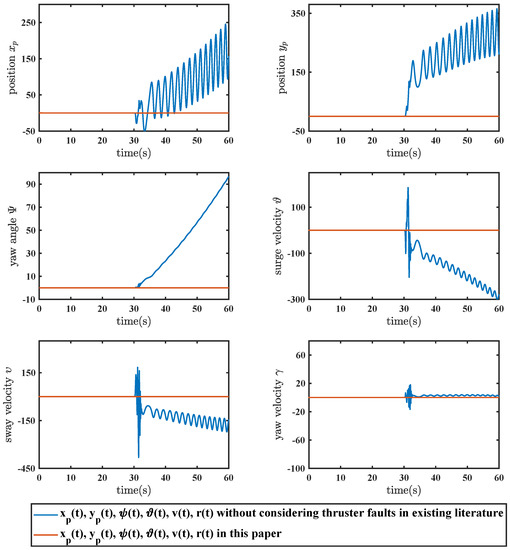
Figure 4.
Comparison of system responses with a normal controller and using the techniques developed in this paper.
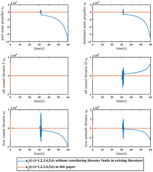
Figure 5.
Comparison of controller responses with a normal controller and using the techniques developed in this paper.
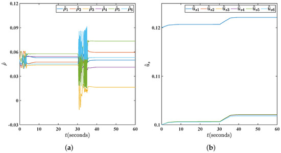
Figure 6.
(a) Responses of parameter using the proposed methodology in fault case with . (b) Responses of parameter using the proposed methodology in fault case with .
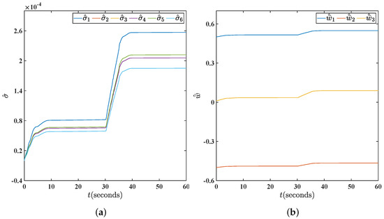
Figure 7.
(a) Responses of parameter using the proposed methodology in fault case with . (b) Responses of parameter using the proposed methodology in fault case with .
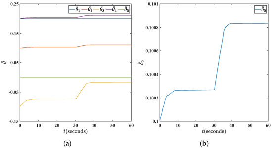
Figure 8.
(a) Responses of parameter using the proposed methodology in fault case with . (b) Responses of parameter using the proposed methodology in fault case with .
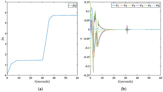
Figure 9.
(a) Responses of parameter using the proposed methodology in fault case with . (b) System responses using the controller developed in this paper with different dominant wave strength coefficient, damping coefficient, and wave encounter frequency.
5. Conclusions
In this paper, an FTC scheme using an ISMC methodology with fault information has been proposed for the DP of a UMV with thruster faults. The nonlinear terms in the T-S fuzzy model have been approximated by the FLS to achieve a tradeoff between resolution and complexity. Moreover, the fault information has been used in the design of the ISM surface in the ISMC of the above UMV DP model, ensuring that the ISMC can further reduce the conservatism and obtain better robustness while maintaining the dynamic performance of the UMV system in severe sea conditions. The validity of our approach has been demonstrated by simulation for a vehicle with realistic parameters.
Author Contributions
Conceptualization, L.-Y.H. and Y.W.; methodology, L.-Y.H. and Y.W.; software, Y.W.; validation, Y.W. and L.-Y.H.; formal analysis, Y.W.; investigation, Y.W.; resources, L.-Y.H., T.L. and C.L.P.C.; data curation, Y.W.; writing—original draft preparation, Y.W.; writing—review and editing, Y.W.; visualization, Y.W.; supervision, L.-Y.H.; project administration, L.-Y.H.; funding acquisition, L.-Y.H., T.L. and C.L.P.C. All authors have read and agreed to the published version of the manuscript.
Funding
This work is supported in part by the National Natural Science Foundation of China (under Grant Nos. 51939001, 52171292, 61976033, 62003069); the LiaoNing Revitalization Talents Program (under Grant Nos. XLYC1908018, XLYC1807046); Dalian Outstanding Young Talents Program (under Grant No.2022RJ05), the Science and Technology Development Fund, Macau SAR (File no. SKL-IOTSC-2018-2020, 0018/2019/AKP).
Institutional Review Board Statement
Not applicable.
Informed Consent Statement
Not applicable.
Data Availability Statement
Not applicable.
Conflicts of Interest
The author declares no conflict of interest.
References
- Roberts, G.N.; Sutton, R. Advances in Unmanned Marine Vehicles, 1st ed.; Institution of Engineering and Technology: London, UK, 2006. [Google Scholar]
- Wang, Y.L.; Han, Q.L. Network-based modelling and dynamic output feedback control for unmanned marine vehicles in network environments. Automatica 2018, 91, 43–53. [Google Scholar] [CrossRef]
- Kahveci, N.E.; Ioannou, P.A. Adaptive steering control for uncertain ship dynamics and stability analysis. Automatica 2013, 49, 685–697. [Google Scholar] [CrossRef]
- Zereik, E.; Bibuli, M.; Mišković, N.; Ridao, P.; Pascoal, A. Challenges and future trends in marine robotics. Annu. Rev. Control 2018, 46, 350–368. [Google Scholar] [CrossRef]
- Wang, L.; Wu, Q.; Liu, J.; Li, S.; Negenborn, R.R. State-of-the-art research on motion control of maritime autonomous surface ships. J. Mar. Sci. Eng. 2019, 7, 438. [Google Scholar] [CrossRef]
- Peng, Z.; Wang, J.; Wang, D.; Han, Q.L. An Overview of Recent Advances in Coordinated Control of Multiple Autonomous Surface Vehicles. IEEE Trans. Ind. Informatics 2021, 17, 732–745. [Google Scholar] [CrossRef]
- Ning, J.; Li, T.; Chen, C.P. Neuro-adaptive distributed formation tracking control of under-actuated unmanned surface vehicles with input quantization. Ocean. Eng. 2022, 265, 112492. [Google Scholar] [CrossRef]
- Wang, Y.L.; Han, Q.L. Network-Based Heading Control and Rudder Oscillation Reduction for Unmanned Surface Vehicles. IEEE Trans. Control Syst. Technol. 2017, 25, 1609–1620. [Google Scholar] [CrossRef]
- Katayama, H.; Aoki, H. Straight-Line Trajectory Tracking Control for Sampled-Data Underactuated Ships. IEEE Trans. Control Syst. Technol. 2014, 22, 1638–1645. [Google Scholar]
- Li, T.; Zhao, R.; Chen, C.L.P.; Fang, L.; Liu, C. Finite-Time Formation Control of Under-Actuated Ships Using Nonlinear Sliding Mode Control. IEEE Trans. Cybern. 2018, 48, 3243–3253. [Google Scholar] [CrossRef]
- Hassani, V.; Sørensen, A.J.; Pascoal, A.M.; Athans, M. Robust Dynamic Positioning of offshore vessels using mixed-μ synthesis modeling, design, and practice. Ocean. Eng. 2017, 129, 389–400. [Google Scholar] [CrossRef]
- Du, J.; Hu, X.; Krstić, M.; Sun, Y. Robust dynamic positioning of ships with disturbances under input saturation. Automatica 2016, 73, 207–214. [Google Scholar] [CrossRef]
- Gao, X.; Li, T.; Shan, Q.; Xiao, Y.; Yuan, L.; Liu, Y. Online optimal control for dynamic positioning of vessels via time-based adaptive dynamic programming. J. Ambient. Intell. Humaniz. Comput. 2019, 1–13. [Google Scholar] [CrossRef]
- Li, W.; Sun, Y.; Chen, H.; Wang, G. Model predictive controller design for ship dynamic positioning system based on state-space equations. J. Mar. Sci. Technol. 2017, 22, 426–431. [Google Scholar] [CrossRef]
- Gao, X.; Bai, W.; Li, T.; Yuan, L.; Long, Y. Broad learning system-based adaptive optimal control design for dynamic positioning of marine vessels. Nonlinear Dyn. 2021, 105, 1593–1609. [Google Scholar] [CrossRef]
- Mendel, J.M. Fuzzy logic systems for engineering: A tutorial. Proc. IEEE 1995, 83, 345–377. [Google Scholar] [CrossRef]
- Wang, Y.; Li, T.; Wu, Y.; Yang, X.; Chen, C.; Long, Y.; Yang, Z.; Ning, J. L∞ Fault Estimation and Fault-Tolerant Control for Nonlinear Systems by T-S Fuzzy Model Method with Local Nonlinear Models. Int. J. Fuzzy Syst. 2021, 23, 1714–1727. [Google Scholar] [CrossRef]
- Ho, W.H.; Chen, S.H.; Chou, J.H. Optimal control of Takagi-Sugeno fuzzy-model-based systems representing dynamic ship positioning systems. Appl. Soft Comput. 2013, 13, 3197–3210. [Google Scholar] [CrossRef]
- Ngongi, W.E.; Du, J.; Wang, R. Robust fuzzy controller design for dynamic positioning system of ships. Int. J. Control Autom. Syst. 2015, 13, 1294–1305. [Google Scholar] [CrossRef]
- Wang, Y.L.; Han, Q.L.; Fei, M.R.; Peng, C. Network-Based T-S Fuzzy Dynamic Positioning Controller Design for Unmanned Marine Vehicles. IEEE Trans. Cybern. 2018, 48, 2750–2763. [Google Scholar] [CrossRef]
- Yu, X.N.; Hao, L.Y. Integral sliding mode fault tolerant control for unmanned surface vessels with quantization: Less iterations. Ocean. Eng. 2022, 260, 111820. [Google Scholar] [CrossRef]
- Lv, T.; Zhou, J.; Wang, Y.; Gong, W.; Zhang, M. Sliding mode based fault tolerant control for autonomous underwater vehicle. Ocean. Eng. 2020, 216, 107855. [Google Scholar] [CrossRef]
- Zhang, G.; Gao, S.; Li, J.; Zhang, W. Adaptive neural fault-tolerant control for course tracking of unmanned surface vehicle with event-triggered input. Proc. Inst. Mech. Eng. Part I J. Syst. Control. Eng. 2021, 235, 1594–1604. [Google Scholar] [CrossRef]
- Blanke, M.; Izadi-Zamanabadi, R.; Lootsma, T.F. Fault monitoring and re-configurable control for a ship propulsion plant. Int. J. Adapt. Control. Signal Process. 1998, 12, 671–688. [Google Scholar] [CrossRef]
- Baldini, A.; Felicetti, R.; Freddi, A.; Longhi, S.; Monteriù, A. Actuator fault tolerant control via active fault diagnosis for a remotely operated vehicle. IFAC Pap. 2022, 55, 310–316. [Google Scholar] [CrossRef]
- Hao, L.Y.; Zhang, H.; Guo, G.; Li, H. Quantized Sliding Mode Control of Unmanned Marine Vehicles: Various Thruster Faults Tolerated With a Unified Model. IEEE Trans. Syst. Man Cybern. Syst. 2021, 51, 2012–2026. [Google Scholar] [CrossRef]
- Zhang, G.; Chu, S.; Huang, J.; Zhang, W. Robust adaptive fault-tolerant control for unmanned surface vehicle via the multiplied event-triggered mechanism. Ocean. Eng. 2022, 249, 110755. [Google Scholar] [CrossRef]
- Hao, L.Y.; Zhang, H.; Li, T.S.; Lin, B.; Chen, C.L.P. Fault Tolerant Control for Dynamic Positioning of Unmanned Marine Vehicles Based on T-S Fuzzy Model With Unknown Membership Functions. IEEE Trans. Veh. Technol. 2021, 70, 146–157. [Google Scholar] [CrossRef]
- Fossen, T.; Sagatun, S.; Sørensen, A. Identification of dynamically positioned ships. Control Eng. Pract. 1996, 4, 369–376. [Google Scholar] [CrossRef]
- Hao, L.Y.; Yu, Y.; Li, T.S.; Li, H. Quantized Output-Feedback Control for Unmanned Marine Vehicles With Thruster Faults via Sliding-Mode Technique. IEEE Trans. Cybern. 2022, 52, 9363–9376. [Google Scholar] [CrossRef]
- Zhou, K.; Doyle, J.C.; Glover, K. Robust Optim. Control, 1st ed.; Prentice-Hall, Inc.: Hoboken, NJ, USA, 1996. [Google Scholar]
- Gao, X.; Li, T.; Yuan, L.; Bai, W. Robust Fuzzy Adaptive Output Feedback Optimal Tracking Control for Dynamic Positioning of Marine Vessels with Unknown Disturbances and Uncertain Dynamics. Int. J. Fuzzy Syst. 2021, 23, 2283–2296. [Google Scholar] [CrossRef]
- Castanos, F.; Fridman, L. Analysis and design of integral sliding manifolds for systems with unmatched perturbations. IEEE Trans. Autom. Control 2006, 51, 853–858. [Google Scholar] [CrossRef]
- Edwards, C.; Spurgeon, S. Sliding Mode Control: Theory and Applications, 1st ed.; CRC Press: London, UK, 1998. [Google Scholar]
- Manzanilla, A.; Ibarra, E.; Salazar, S.; Zamora, Á.E.; Lozano, R.; Munoz, F. Super-twisting integral sliding mode control for trajectory tracking of an Unmanned Underwater Vehicle. Ocean. Eng. 2021, 234, 109164. [Google Scholar] [CrossRef]
- Banza, A.T.; Tan, Y.; Mareels, I. Integral sliding mode control design for systems with fast sensor dynamics. Automatica 2020, 119, 109093. [Google Scholar] [CrossRef]
- Li, P.; Liu, D.; Baldi, S. Adaptive integral sliding mode control in the presence of state-dependent uncertainty. IEEE ASME Trans. Mechatronics 2022, 27, 3885–3895. [Google Scholar] [CrossRef]
- Qi, W.; Gao, X.; Ahn, C.K.; Cao, J.; Cheng, J. Fuzzy integral sliding-mode control for nonlinear semi-Markovian switching systems with application. IEEE Trans. Syst. Man Cybern. Syst. 2020, 52, 1674–1683. [Google Scholar] [CrossRef]
Disclaimer/Publisher’s Note: The statements, opinions and data contained in all publications are solely those of the individual author(s) and contributor(s) and not of MDPI and/or the editor(s). MDPI and/or the editor(s) disclaim responsibility for any injury to people or property resulting from any ideas, methods, instructions or products referred to in the content. |
© 2023 by the authors. Licensee MDPI, Basel, Switzerland. This article is an open access article distributed under the terms and conditions of the Creative Commons Attribution (CC BY) license (https://creativecommons.org/licenses/by/4.0/).