Article

High-Resolution Model of Clew Bay—Model Set-Up and Validation Results

1
Marine Institute, Galway, Ireland
2
Oceanography Department, Faculty of Science, Alexandria University, Alexandria 21500, Egypt
3
Department of Marine Sciences, School of the Environment, University of the Aegean, 81100 Mytilene, Greece
4
Environmental Protection Agency (EPA), Castlebar, Ireland
*
Author to whom correspondence should be addressed.
J. Mar. Sci. Eng. 2023, 11(2), 362; https://doi.org/10.3390/jmse11020362
Submission received: 13 January 2023 / Revised: 31 January 2023 / Accepted: 1 February 2023 / Published: 6 February 2023
(This article belongs to the Special Issue Hydrodynamic Circulation Modelling in the Marine Environment)

Abstract

:
Clew Bay is an important aquaculture production area in Ireland. In this study, we focused on a high-resolution simulation of the Clew Bay region based on a regional ocean modeling system (ROMS). Freshwater discharges from eight rivers are included in the model and a wetting–drying scheme has been implemented. The Clew Bay model simulation was validated and calibrated with available observations (e.g., acoustic Doppler current profiler (ADCP), vertical salinity and temperature profiles, and a tide gauge) in the geographic area of the model domain. High correlations were found between the model data and observed temperature, salinity and water levels, along with small root mean square errors. This indicates that the model is able to reproduce the oceanographic phenomena in the study area. The Taylor diagram analysis showed a high correlation coefficient (R = 0.99) between the observed bottom temperature in the Inner Bay and Clew Bay model, along with a small centered root mean square error (RMSD = 0.5 °C). High correlation coefficients (R > 0.80) were found between the model and the two ADCPs for the zonal current component. There was a resemblance in structure between the model and the observed salinity profiles, indicating that freshwater was correctly implemented in the model. Moreover, the correlation coefficient between the model and the tidal sea surface height (SSH) was 0.99, with an RMSD of 0.09 m. We discovered that wind direction and speed had a significant impact on the bay’s water inflow rate. The model outputs can be used to provide scientists, fishermen, and decision-makers with hydrodynamic information on ocean conditions in the bay.

1. Introduction

Clew Bay is a large bay with an area of about 176 km2 (i.e., 16 km from east to west and 11 km from north to south) situated on the west coast of Ireland, characterized by a large number of islands (see Figure 1). The bay is bounded by Croagh Patrick Mountains to the south and Achill Island to the north (Figure 1). The islands in Clew Bay are partially drowned drumlins, i.e., elongated, steeply sloping hills that were sometimes called “whalebacks” [1]. They were formed when glaciers reshaped the landscape during the last ice age [1]. Several of the hills on the mainland around the bay are similar drumlins [2]. These glacial formations vary considerably in size, ranging from large islands on which residences and pastures stand to small mounds on the seafloor [1]. The numerous islands give rise to shallow straits and lagoons through which deep channels flow [2]. Erosion of existing and submerged drumlins with their coarse glacial deposits gives rise to a heterogeneous sediment environment [2,3]. Clew Bay has 365 islands, the largest of which, Clare Island, protects the entrance to the sheltered bay [4], as shown in Figure 1.
Clew Bay is an important national region responsible for aquaculture (i.e., finfish farming, oyster farming, mussels, and others) industry in Ireland [5]. In 2020, there were 22 aquaculture-related businesses in Clew Bay [6], the vast majority of which were involved in oyster farming, although shellfish and finfish farming are also represented locally (https://bim.ie/wp-content/uploads/2022/05/Clew-Bay-Report-SPREADS.pdf; accessed on 20 December 2022). Finfish and oyster farming extends from the Westport River to the Burrishoole Fishery (Loughs Feagh and Furnace) near Newport and is an important national region for aquaculture [6] (Figure 1).
There is a need for an understanding of the hydrodynamic properties of the Clew Bay region by a wide range of stakeholders, e.g., scientists working on salmon migration. To date, there are no published modeling studies for Clew Bay. As regards other recent modeling studies of Irish waters, the set-up and validation results of a high-resolution numerical operational model developed at the Irish Marine Institute covering the north-east Atlantic with emphasis on Irish waters were presented in [7]. The model is based on ROMS with a horizontal resolution of 1 km and runs operationally. The meanders and eddies in the model domain were well resolved. The authors attribute this to the high resolution of the model and detailed bathymetry in the study area. In addition, Ref. [8] has presented a high-resolution (1 km) 3D ocean model based on ROMS for south-western Irish waters. The simulation of the Irish hindcast model was validated and calibrated with available observations in the geographic domain of the model. The model has been shown to be robust when compared to observed vertical temperature and salinity profiles.
Furthermore, in [9], a 3D model of the coastal ocean was created using simple equations for Bantry Bay. The model was developed, validated, and implemented operationally. The authors have found some other modeling studies of the Irish shelf waters, e.g., [10,11,12,13,14,15,16,17,18,19]. Moreover, in [20], the preliminary results of a high-resolution 3D numerical simulation with a wetting and drying scheme based on the regional ocean modeling system (ROMS) were used to study the tidal circulation in Kilmakilloge Harbour. This bay is located on the southern shore of Kenmare Harbour in the south-west of Ireland. The model showed good skill and a high correlation coefficient with respect to the available observations, especially for temperature and tides. However, the model overestimated mixing in Kilmakilloge Harbour.
To the best of the authors’ knowledge, the presented model is the first 3D numerical model developed for Clew Bay. This study reports the validation results of the preoperational model. The model was initialized on 7 June 2017 and ran until 1 January 2019. The model has a horizontal resolution of 80 m and 15 vertical sigma levels. The model was validated using currents recorded by an acoustic Doppler current profiler (ADCP), temperature and salinity profiles from the Irish Environmental Protection Agency (EPA) Ireland website (www.epa.ie/hydronet/#Water%20Levels; accessed on 25 December 2022), and water level records from a tide gauge. Section 2 describes the model implementation and nesting procedures. Section 3 presents the validation against observational data, describes the general circulation in the Clew Bay region, provides estimates of the net flow, and discusses the results before presenting the conclusions in the last section.

2. Model Design, Description and Implementation

The model is based on version 3.7 of the code regional ocean modeling system [21]. All model equations are written in rectangular coordinates and include spatially and temporally varying horizontal eddy viscosity and diffusion coefficients [22]. Orthogonal curved coordinates on an Arakawa “C” grid are used in the horizontal while utilizing a terrain-following coordinate in the vertical. The Clew Bay model has a horizontal grid with a resolution of 80 × 80 m and 15 vertical layers. The terrain-following vertical layers coordinate parameters are as follows: the vertical transform is 2, the vertical stretching is 4, the critical depth (Tcline) is equal to 100 m, the surface stretching parameter (Theta_s) is equal to 0 and the bottom stretching parameter (Theta_b) is equal to 0. The projection of the model grid is rotated with a 2D angle varied from 0° to 10°. The high-resolution bathymetry of the Clew Bay model is from Ireland’s Integrated Mapping for the Sustainable Development of Ireland’s Marine Resource (INFOMAR) database (www.infomar.ie; accessed on 19 June 2022) and the European Marine Observation and Data Network (EMODnet) bathymetric dataset (https://www.emodnet-bathymetry.eu/; accessed on 10 September 2022). Minimal smoothing of the bathymetry was performed using a linear programming method [23]. To reduce pressure gradient errors, we smoothed the model bathymetry using Beckman and Haidvogel rx0 factor [24,25]. Beckman and Haidvogel’s dimensionless rx0 factor did not exceed 0.2 in any of the model grid points. The model also has a wetting and drying scheme according to [26]. The scheme specifies that some points of the ocean grid may be completely “wet” or “dry”. These “dry” points may not have zero depth; instead, they are covered by a thin film of water so that the equations of motion can be calculated at all grid points [27]. The direction of flow is determined at each of the faces of a tracer cell, and the flow and velocity through the face are set to zero if the depth of the upstream tracer cell is less than or equal to a user-specified critical depth Dcrit [26,27]. We have defined the Dcrit to 0.25 m. The turbulence mixing scheme of the model is a k-ε parameterization implemented by the generic length scale (GLS) scheme [28,29]. The turbulence closure parameters for the k-ε (GLS) scheme defined for the Clew Bay model are shown in Table 1. An upstream third-order scheme with implicit mixing was used for the horizontal advection of momentum [30], whilst a multidimensional positive definite advection transport algorithm (MPDATA) was used for horizontal and vertical advection of tracers [31]. Bottom stress is applied using the logarithmic “wall law” with a constant roughness length of 0.01 m.
The Marine Institute’s operational model for the north-east Atlantic (NEA _ROMS) provides initial conditions for the entire Clew Bay model domain and lateral conditions for the three open boundaries [7]. The initial and boundary parameters of the model include temperature, salinity, baroclinic, and barotropic velocity components, and sea surface height. The temporal resolution of the boundary conditions is 10 min and includes the tidal signal. The nesting was designed so that the volume transport across the open boundary of the nested model matches the volume transport of the NEA _ROMS model; this technique was described in [7].
The atmospheric data for the computation of the surface forcing are taken from the global high-resolution (0.125°) atmospheric model run by the European Centre for Medium Range Weather Forecasts (ECMWF) at a 3-h frequency. The atmospheric fields used are air temperature, relative humidity, wind speed at 10 m height, mean sea level pressure, total cloud cover, total precipitation, surface solar radiation, and net longwave radiation. Wind stress, heat fluxes, and evaporation rates are calculated using an interactive mass formula that uses atmospheric data, as described in [8]. Daily averaged freshwater discharges were specified for eight major rivers (see Table 2). Data for four rivers were obtained from the European Hydrological Forecasts for the Environment (Swedish Meteorological and Hydrological Institute (E-HYPE SMHI)); https://hypeweb.smhi.se/explore-water/historical-data/europe-time-series/; accessed on 20 September 2022) [32], while the data for the remaining rivers were obtained from the Irish Environmental Protection Agency (EPA) Ireland website (https://epawebapp.epa.ie/hydronet/#Water%20Levels; accessed on 20 December 2022). Daily climatological flows for the four rivers in the E- HYPE (Owenwee, Burrishoole, Owengrave, and Mayour) were calculated from available flow time series over a 30-year period (1981–2010). Daily flow rates for the Newport, Westport, Owennabrockagh, and Bunowen rivers were determined from time series from EPA for a 10-year period (2006–2016). The salinity of incoming freshwater was set to zero, and temperature was calculated from monthly temperatures for the period 2000–2010, available at HYPE-SMHI: (https://hypeweb.smhi.se/explore-water/historical-data/europe-time-series/; accessed on 25 September 2022).
The model was initialized on 7 June 2017 and ran until 1 January 2019. The output consists of temperature, salinity, sea surface height, barotropic, and baroclinic velocity fields and is stored in netCDF files in hourly snapshots. In addition, the output is stored at a frequency of 10 min at selected locations in the area for use in model validation.
Data used to validate the 1.5-year hindcast simulation (i.e., June 2017–1 January 2019), included two ADCPs, four EPA temperature and salinity profiles, and Roonagh Tide Gauge Station (see Figure 1).
ADCP is a hydro-acoustic current measurement device anchored near the bottom, similar to sonar, and used to measure current velocities over a range of depths using the Doppler effect of sound waves backscattered from particles in the water column [33]. Two ADCPs were deployed from 25 July to 20 December 2017, and measured currents at a frequency of 12 min. The locations of the ADCPs were north of Clare Island at 9.9684833° W, 53.841317° N, where the local water depth is around 42 m, and in the inner bay at 9.6707833° W, 53.863817° N, where the local water depth is about 18 m (see Figure 1). For Clare Island, the ADCP has 39 bins to measure current at various depth intervals, with the 1-m interval beginning at 3.72 m and ending at 41.72 m, while for the inner bay, the ADCP has 30 bins, with a 0.5 m depth interval beginning at 3.23 m and ending at 17.73 m. The two ADCPs included a thermistor placed between the ADCP transducers to measure seawater temperature. Validation was performed for the temperature and barotropic velocity components over the above time period. Comparison with the barotropic velocity components of the ADCPs rather than the absolute velocity components of the ADCPs reduces the uncertainties in the ADCP velocities, as described in [34,35,36]. We calculated the ADCP barotropic velocity components by integrating the ADCP velocity components related to the water column resolved by the ADCP.
Roonagh Tide Gauge Station data for water levels are from 14 August 2017 to 2 January 2018 and were obtained from the Irish National Tide Gauge Network (https://data.gov.ie/dataset/irish-national-tide-gauge-network; accessed on 15 Obtober 2022). This tide gauge station is located at Roonagh Pier in the south of the island of Clare and recorded water levels at 6-min intervals from 14 August 2017 to 2 January 2018. Harmonic analysis of the observed and modeled sea surface height (SSH) time series was performed using the T-TIDE software in MATLAB [37]. The objective of the analysis is to compare the modeled and measured values of the main tidal constituents (magnitude and phase angle).
Data for the temperature and salinity profiles are collected as part of the EPA national water quality monitoring programme (https://www.epa.ie/publications/monitoring--assessment/freshwater--marine/irelands-national-water-framework-directive-monitoring-programme-2019–2021.php accessed on 15 November 2022). Data were collected using vertical profiles at each station. A data sonde was lowered from the surface to the bottom of the water column and each parameter is recorded at ~1 m intervals where total depth was less than 10 m and ~2 m where the total depth was >10 m. The data sondes used were Hydrolab DS5 or Hydrolab HL7 sondes. Each instrument was equiped with sensors to record depth (m), salinity, pH, optical dissolved oxygen (% saturation), turbidity (NTU), and chlorophyll A(µg/L). Data were recorded to a Hydrolab Surveyor handheld datalogger. Salinity measurements were calibrated against KCL standards of known conductivity. The EPA station locations are listed in Table 3.
Hourly historical wind data from 1 January 2000 to 31 December 2021 were retrieved from the Irish Meteorological Service (Met Éireann) (https://www.met.ie/climate/available-data/historical-data accessed on 31 January 2023). The wind station is located in the town of Belmullet on Achill Island north of Clew Bay (Figure 1). The wind data include wind speed in knots and wind direction in degrees, and were used to plot the wind rose using the wind rose software in MATLAB [38].
The Taylor diagram [39] was used to show the validation of the model results. The Taylor diagram provides a concise statistical summary of the agreement between patterns (i.e., observations and model) in terms of their correlation (R), their root mean square difference (RMSD), and the ratio of their standard deviations. This ratio is indicated by the location of a point representing the test plot (i.e., model) relative to the reference point (i.e., observations). The reference point is located on the x-axis [39]. RMSD represents the sample standard deviation of the differences between model values and observed values.

3. Results and Discussion

3.1. Validation of the Clew Bay Model against Observations

In this part, we discuss the validation results of the Clew Bay hindcast simulation with available ocean observations described in Section 2.

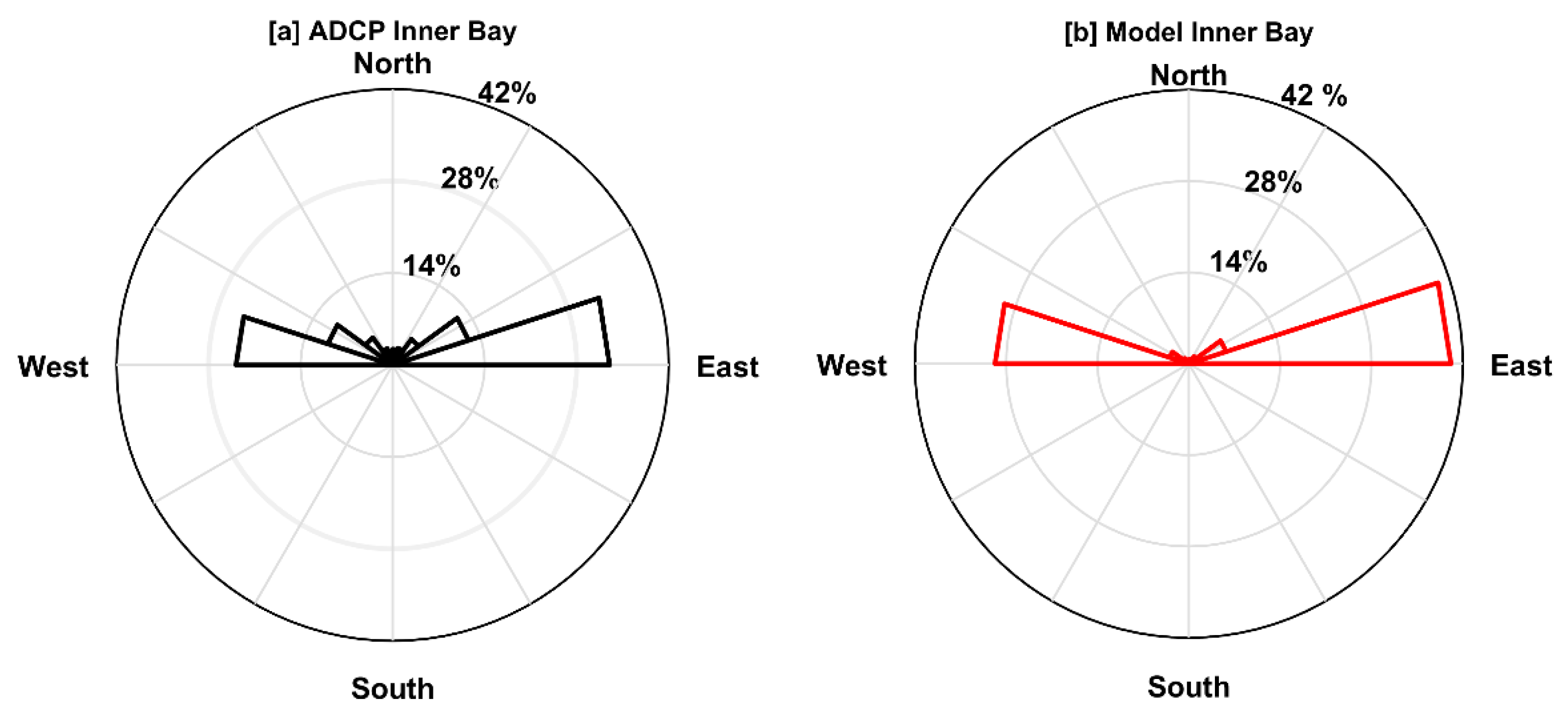
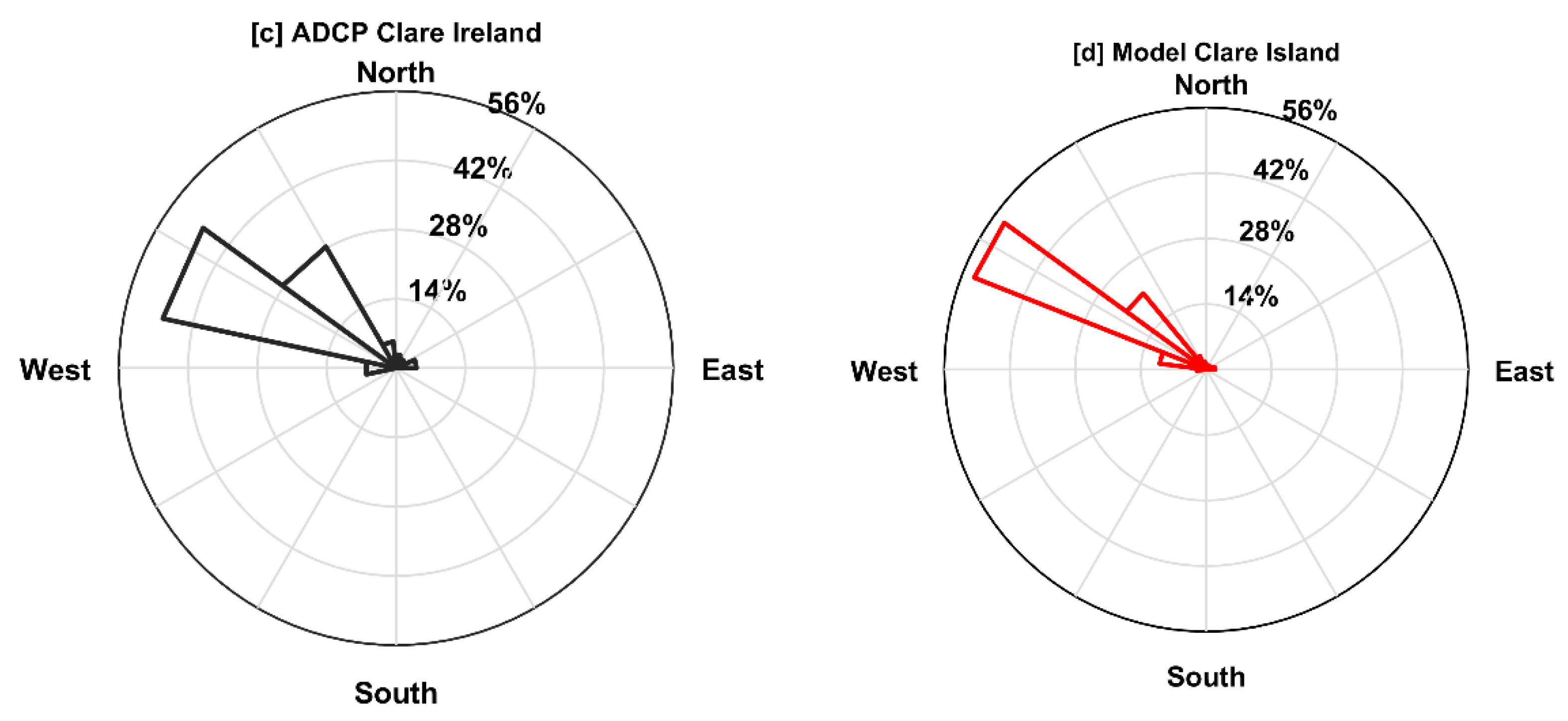
3.1.1. Validation with ADCPs

Figure 2 shows the comparison of the time series between the Clew Bay model and observed bottom temperature in [°C] for the period from 25 July to 20 December 2017. In August and September, the model bottom temperature was about 1.3 °C warmer than the observed temperature in the inner bay, as shown in Figure 2a. This large deviation between the model and observations in bottom temperature occurs only from 25 July to early September but not during the rest of the simulation period. This deviation can be attributed to the necessary spin-up time with some seasonal effects (i.e., the transition from summer to autumn) for the high-resolution (80 m) Clew Bay model. The model was initialized on June 7 and it may require a spin-up time to stabilize and reach an equilibrium solution [40]. The smallest differences (<0.2 °C) between the Clew Bay model and the inner bay observed bottom temperature were detected for the remainder of the inner bay observed period (i.e., September to December 2017 (Figure 2a)). This period shows good agreement between model bottom temperature and observations within Clew Bay. Comparison between the Clew Bay model and the Clare Island observed temperature showed that the model was in good agreement with the observations from 21 September to 25 December 2017 (i.e., differences were less than 0.2 °C), as shown in Figure 2b. The largest temperature differences (>1 °C) between the Clew Bay model and the Clare Island ADCP were observed between 10 and 20 September 2017 (see Figure 2b). During this period, the model was cooler than the Clare Island observations. This may result in excessive vertical mixing of the model with the colder bottom water below. This mixing could be due to tides and winds creating areas of well-mixed water. This can lead to a significant cooling of the simulated temperature.
Figure 3 shows the comparison between the Clew Bay model and observed bottom temperature in the form of a Taylor diagram and is based on a 5-month period from 25 July 2017 to 25 December 2017 with a frequency of 10 min. The Taylor diagram generally shows a very high correlation (i.e., R > 0.95) between the model and observed bottom temperature. Figure 3a shows that the correlation coefficient and centered root mean square difference (RMSD) between the model and observed water temperature in the inner bay are nearly 0.99 and 0.5, respectively. For Clare Island (Figure 3b), the correlation coefficient was 0.97 and the RMSD was nearly 0.53. The Taylor diagram also shows that the simulated bottom temperature variations are close to those observed.
Figure 4a–d presents Taylor diagrams comparing the barotropic velocity components (u, v) between the Clew Bay model and the ADCPs in the inner bay and Clare Island, with the corresponding correlation coefficients and RMSD. The model results show that the model is significantly correlated with the barotropic velocity components (u, v) of the ADCPs over the above time period with a confidence limit of 95%. The correlation coefficients and RMSD between the model and the ADCPs in the inner bay and Clare Island for the eastern u-components were [0.85, 0.14] and [0.81, 0.12], respectively, as shown in Figure 4a,b. For the northern v-components, the correlation coefficients and RMSD between the model and ADCPs are [0.25, 0.03] and [0.82, 0.07], respectively (see Figure 4b). The barotropic velocity components (u, v) of the model for the Clare Island site are closer to the observations than those for the inner bay (Figure 4a,b). This can be attributed to the effect of coastal waves; this feature is not implemented in our model [41]. This coastal wave effect is smaller in the Clare Island area with a depth of about 40 m, but larger in shallow areas such as the inner bay with a depth of 15 m [42]. Another possible reason is that the local variation in the inner bay is not well represented by the model smoothed bathymetry grid. In general, the highest correlation coefficients were found for the u component between the model and ADCPs. The modeled meridional current velocity (v-component) in the inner bay is much weaker than the observed value, which could be the reason for the (poor) correlation of the v-component values.
Figure 5a–d demonstrates the current rose direction of measured and modeled barotropic currents from both ADCP locations for the same time period to give a more intuitive visualization of the current directions and how they are reproduced in the Clew Bay model. There are clear similarities between both ADCPs in the inner bay and Clare Islands with the model. The dominant current directions for the inner bay are east by >28% then to the west >25% from the total current directions. This direction represents the tidal movement during the high and low water, which flows in and out of the Clew Bay.
Figure 5a–d shows the current rose of the measured and modeled barotropic flows from both ADCP sites for the same time period to provide a more intuitive visualization of the flow directions and their reproduction in the Clew Bay model. There are clear similarities between the two ADCPs current directions in the inner bay and Clare Islands with the model. The predominant flow directions for the inner bay are eastward >28% and westward >25% of the total flow directions (Figure 5a,b). These directions represent the tidal movement during high and low tides bringing water into and out of Clew Bay. The predominant flow direction for the Clare Island site is north-west >42% of the total flow direction (see Figure 5c,d). These results indicate that water at this site always flows out of Clew Bay.
Overall, validation of the Clew Bay model with the ADCPs during the deployment period showed good agreement with both temperature and barotropic velocity components.

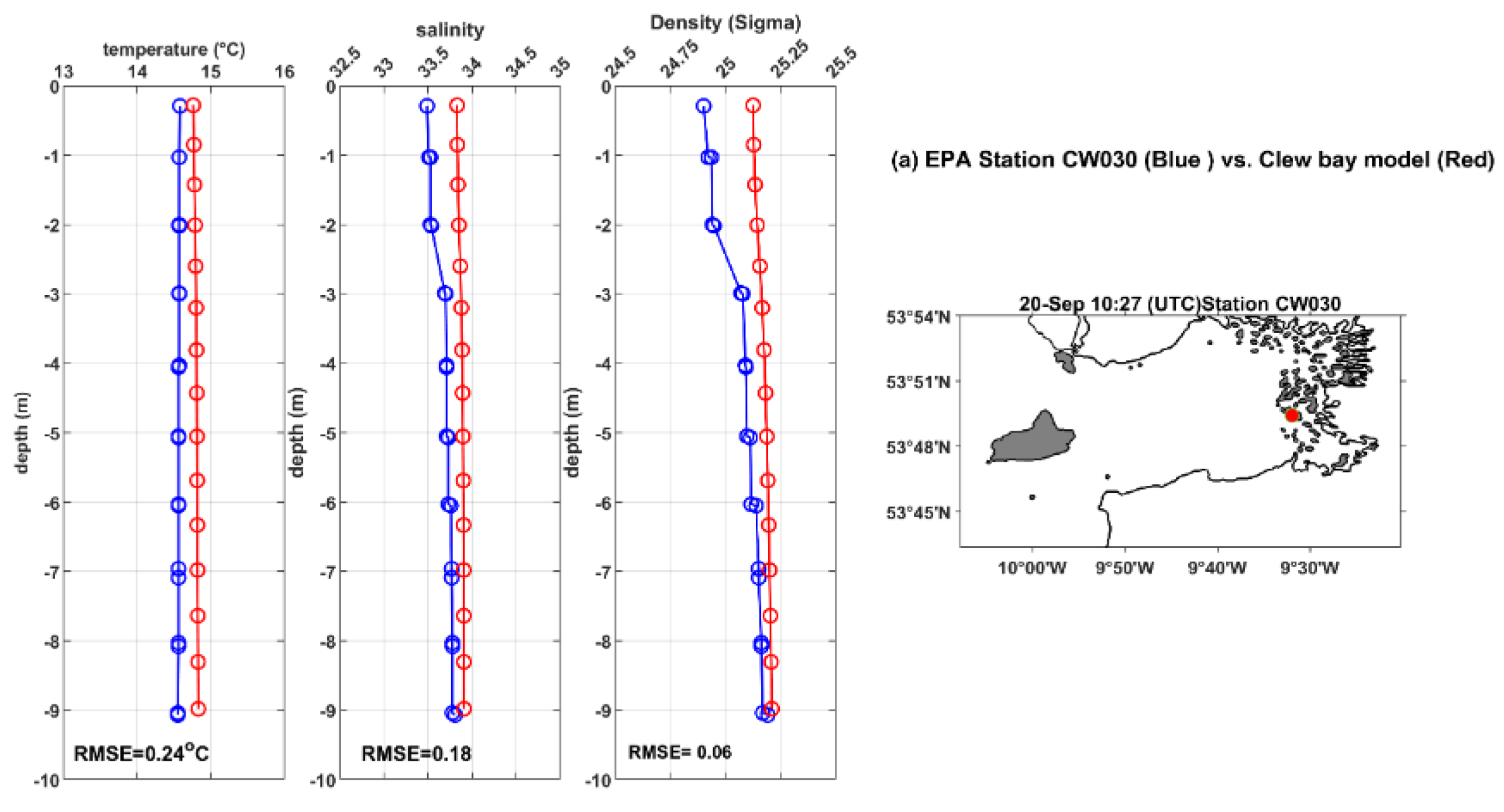
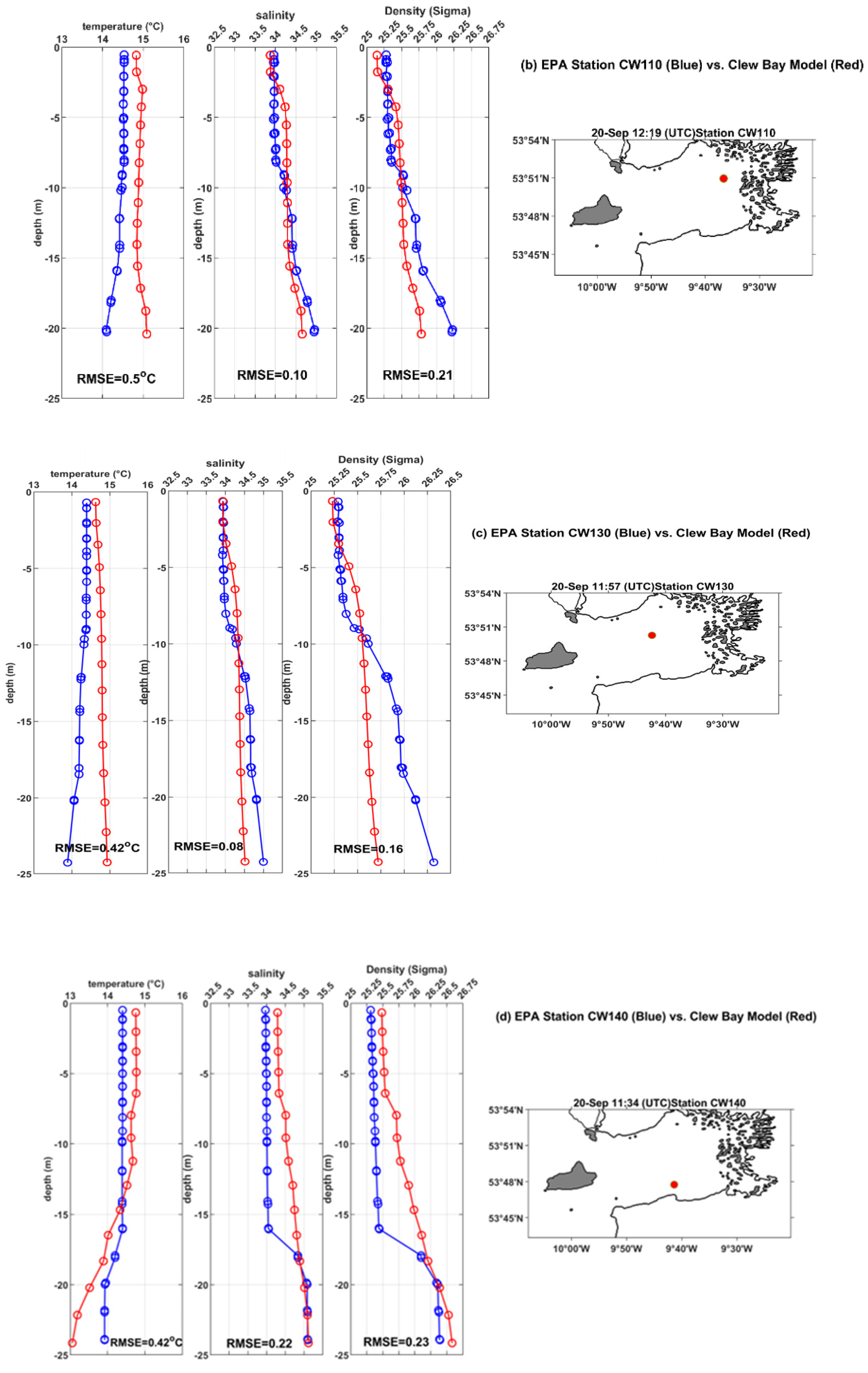
3.1.2. Validation of the Model with In-Situ Temperature and Salinity Vertical Profiles

In this part, we discuss the validation results of the Clew Bay simulation with the available temperature and salinity profiles obtained from the EPA recorded on 20 September 2017 and described in Section 2. Figure 6a–d depicts the validation of simulated temperature, salinity, and density for the profiles at four stations: CW030, CW110, CW130, and CW140. The simulated temperature, salinity, and density profiles are similar to the observations (see Figure 6). The RMSE between model and observations for temperature varies between 0.24 and 0.5 °C. The maximum temperature RMSE is 0.5 °C at station CW110 (Figure 1 and Figure 6b), located in the north of the inner bay, while the minimum RMSE is at a shallow (i.e., depth ~9 m) station CW030 in the south of the inner bay (Figure 1 and Figure 6a). The haloclines and pycnoclines at 2–3 m depth at CW030, at 16–17 m depth at CW140, and at 9–10 m depth at CW130 appear to be missing from the model (Figure 6a–c), which may be an indirect effect of excess vertical mixing of the model due to the use of associated parameters with the k-ε (GLS) scheme for vertical turbulent closure, as described in [43,44]. In general, the vertical structure of salinity in Clew Bay is generally well reproduced by the model (Figure 6). The salinity at the shallow station CW030 is almost homogeneous and shows the same values. The minimum RMSE of salinity (~0.08) is observed at station CW130 almost in the middle of the inner bay (Figure 1 and Figure 6c). The similarity of the structure between the model and the observed salinity indicates the correct implementation of freshwater in the model. Model density agrees with observations at all stations, especially in the upper 10 m, and RMSE varies from 0.06 to 0.23. In summary, the analysis shows that the Clew Bay model is well able to reproduce vertical profiles in the study area.

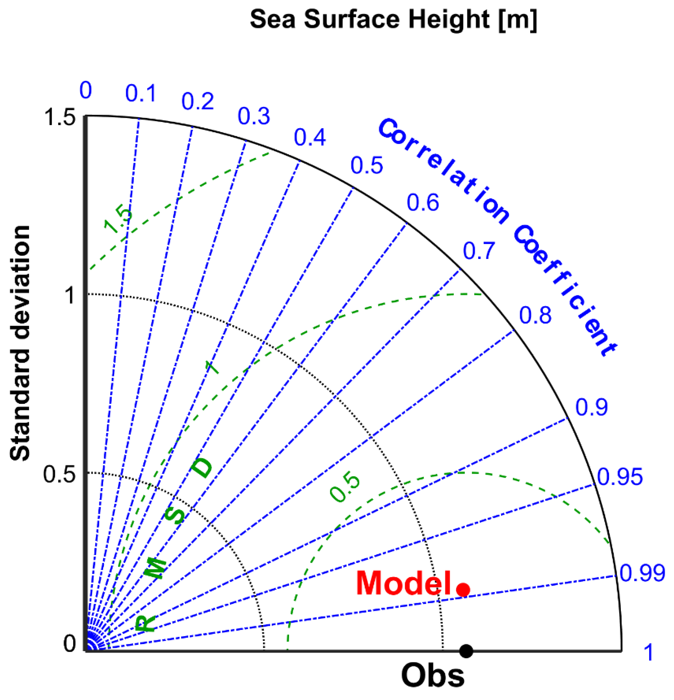
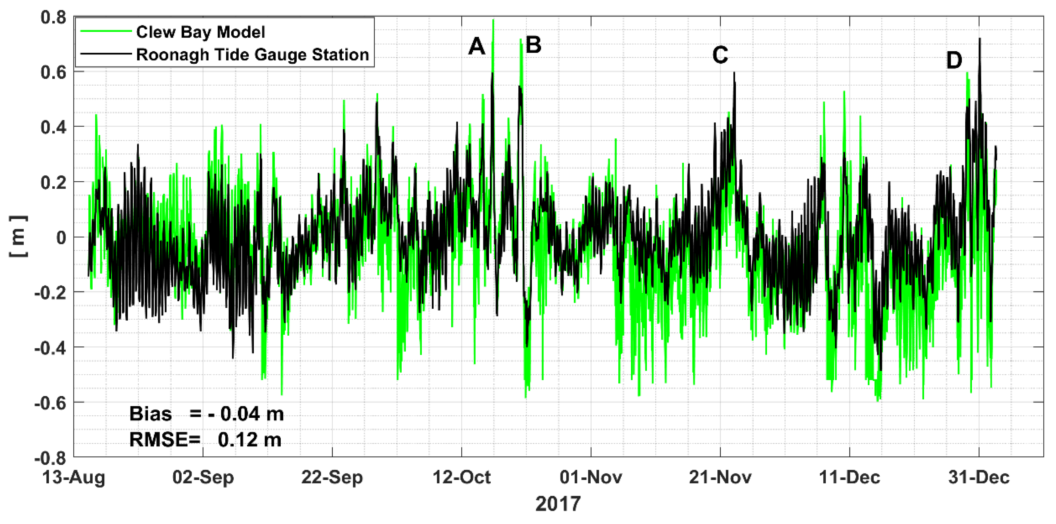
3.1.3. Validation with Roonagh Tide Gauge Station

Figure 7 depicts a statistical comparison between the model and the Roonagh Tide Gauge Station as shown by the Taylor diagram from 14 August 2017 to 2 January 2018. We found that the model was significantly correlated (95% confidence level) with the SSH value of the tide gauge over the above period in the Taylor diagram. The correlation coefficient between the model and the tidal SSH level was 0.99 with an RMSD of 0.09 m. The Taylor diagram also shows that the amplitude of the simulated SSH fluctuations is close to that observed. These results highlight the robustness of the SSH model for Clew Bay, which is probably due to the better boundary condition for the water flow in the model mentioned in [45].
This analysis showed that the tidal signal in the SSH data was dominated by three semidiurnal constituents with three diurnal constituents. The constituents are M2, S2, N2, K1 O1, and Q1. Table 3 shows the comparison between the amplitude and phase angle of the modeled and measured main tidal constituents with the differences between them (model observations). Our analysis show that M2 and S2 are responsible for most of the tides in the area, in agreement with [7,46,47,48,49]. The magnitude differences between the Clew Bay model and the Roonagh tide gauge were very small for all tidal constituents. The amplitude difference varied from 0.05 m for M2 (i.e., less than 4% of the total M2) to [−0.005] for Q1. There were some small differences in phase angle for the K1 and O1 diurnal constituents. The highest phase angle difference was [+9.19°] for constituents K1, while the lowest was [−0.43°] for M2 (see Table 4). The differences between the modeled and observed amplitudes of the constituents showed that the model had good agreement for M2, S2, N2, and Q1. In conclusion, a very good agreement was obtained for all tidal constituents.
Furthermore, the surge component was derived following [37] for observed and modeled data at the Roonagh tide gauge site, and the different statistics are presented. The surge (residual) component of sea level is known as the total water level minus the tide, according to [50]. Figure 8 shows the observed and modeled storm surge at the Roonagh gauge. The Clew Bay model successfully generated the four storm surges (Surge > 0.6 m; A, B, C, and D) on 17 October, 22 October, 23 November, and 31 December 2017 (see Figure 8). The bias between them was [−0.04] m, while the RMSE was 0.12 m.

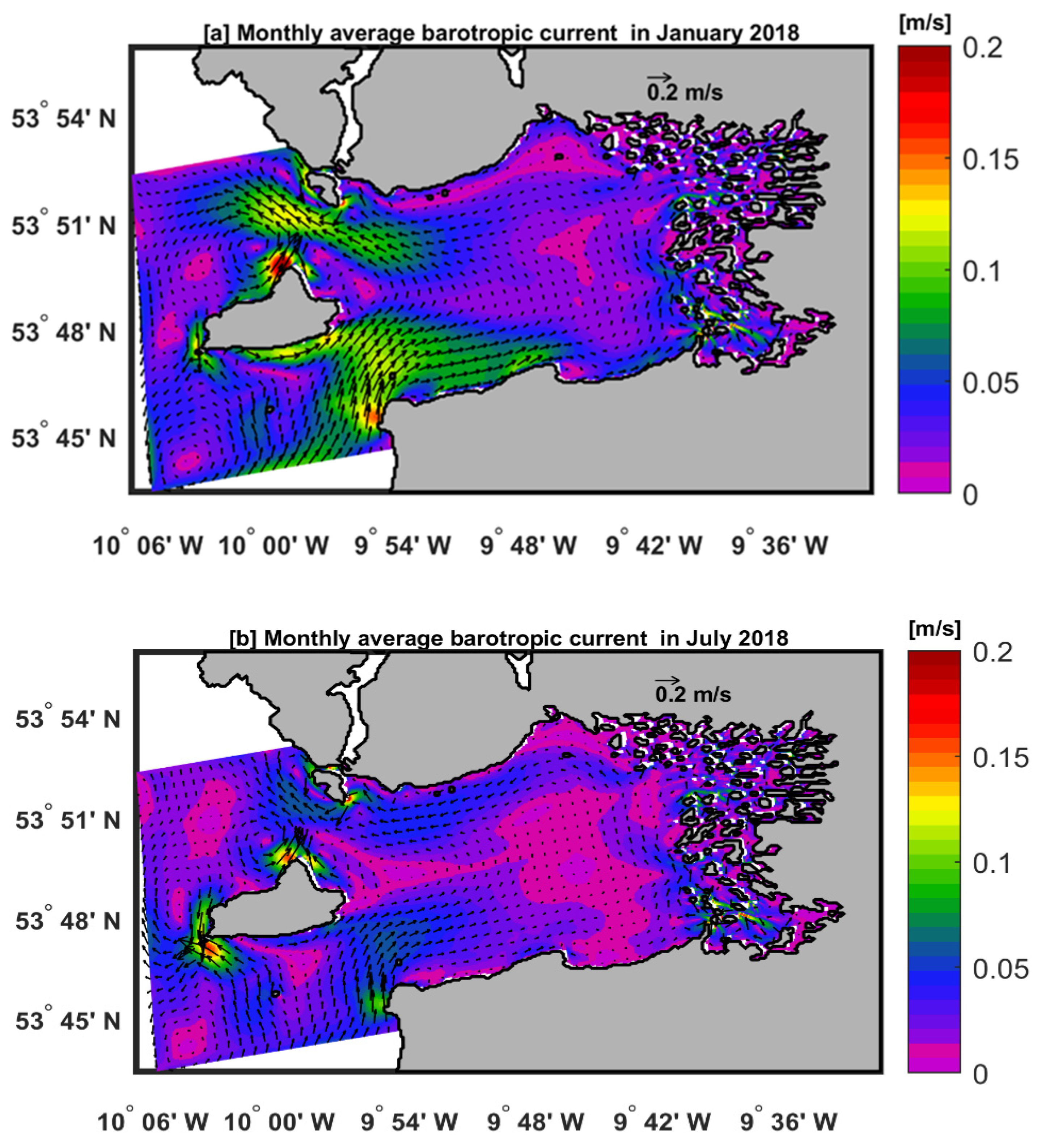
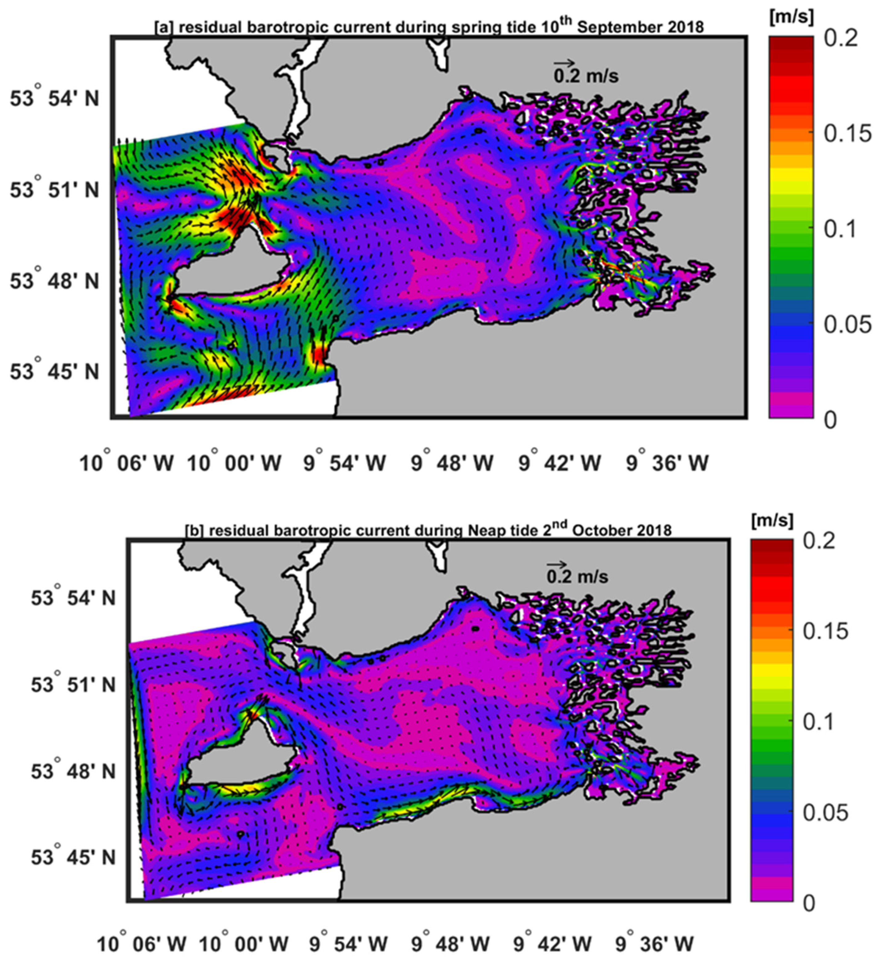
3.2. Clew Bay Current Patterns

Here, we describe the monthly averaged barotropic current patterns in the Clew Bay model during winter, represented by January, and summer, represented by July. In addition, we present the residual barotropic current on 10 September 2018 (spring tide) and 2 October 2018 (neap tide). The residual current is the current with the tidal signal removed and it was approximated here by averaging over 25 h [51,52]. The residual current is the result of several processes such as density-driven current and wind-driven current.
Figure 9a,b shows the monthly water barotropic velocity fields for the Clew Bay model in winter (January) and summer (July). There are similarities between all months in the flow patterns of the Clew Bay main circulation. Water flows into Clew Bay south of Clare Island, while north of Clare Island the flow is outward with a cyclonic (counterclockwise) circulation inside the bay occupying geographic positions 53°51′ N and 10°00′ W. The current entering the bay is deflected to the right due to the Coriolis force. The flow south and north of Clare Island into and out of Clew Bay is relatively stronger in winter (>0.1 m/s) (Figure 9b). This current south and north of Clare Island is weaker in summer (<0.1 m/s) due to less wind.
Figure 10a,b depicts residual currents at spring tide on 10 September 2018 and at neap tide on 2 October 2018. Residual barotropic currents at neap tide in Clew Bay are relatively small (<0.1 m/s) compared to residual barotropic spring tide (>0.1 m/s). The maximum residual barotropic current velocity of about 0.2 [m/s] is located north of Clare Island at a latitude of ~53°50′ N and a longitude of ~10°00′ W (Figure 10a). During the neap tide, a slightly stronger longshore current (~0.1 m/s) flows along the southern coast of Clew Bay (Figure 10b). Overall, the detailed representation of the barotropic ocean currents is due to the high model resolution (80 m), which helps to identify the spatial variation and resolve the small-scale gradient well.

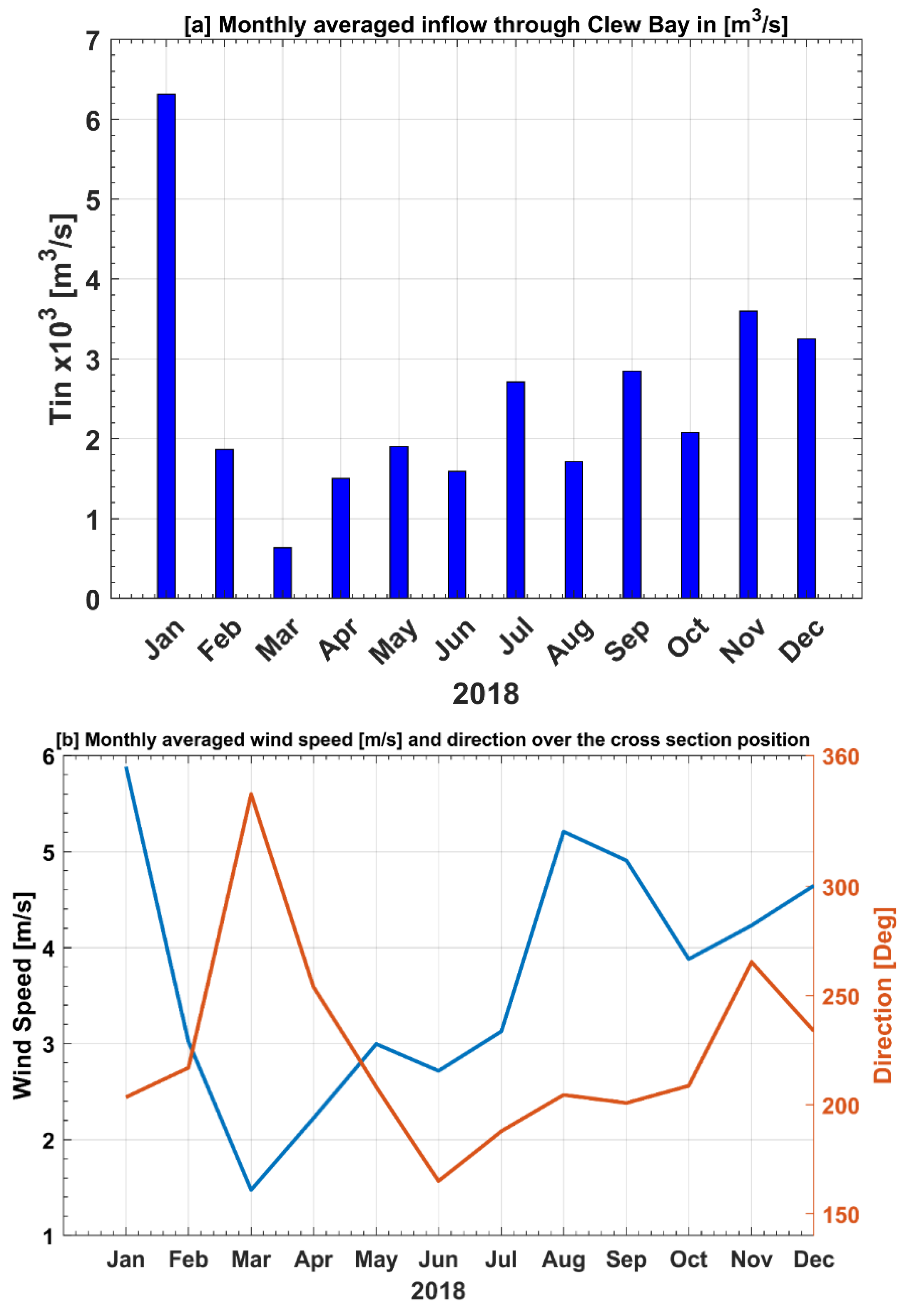
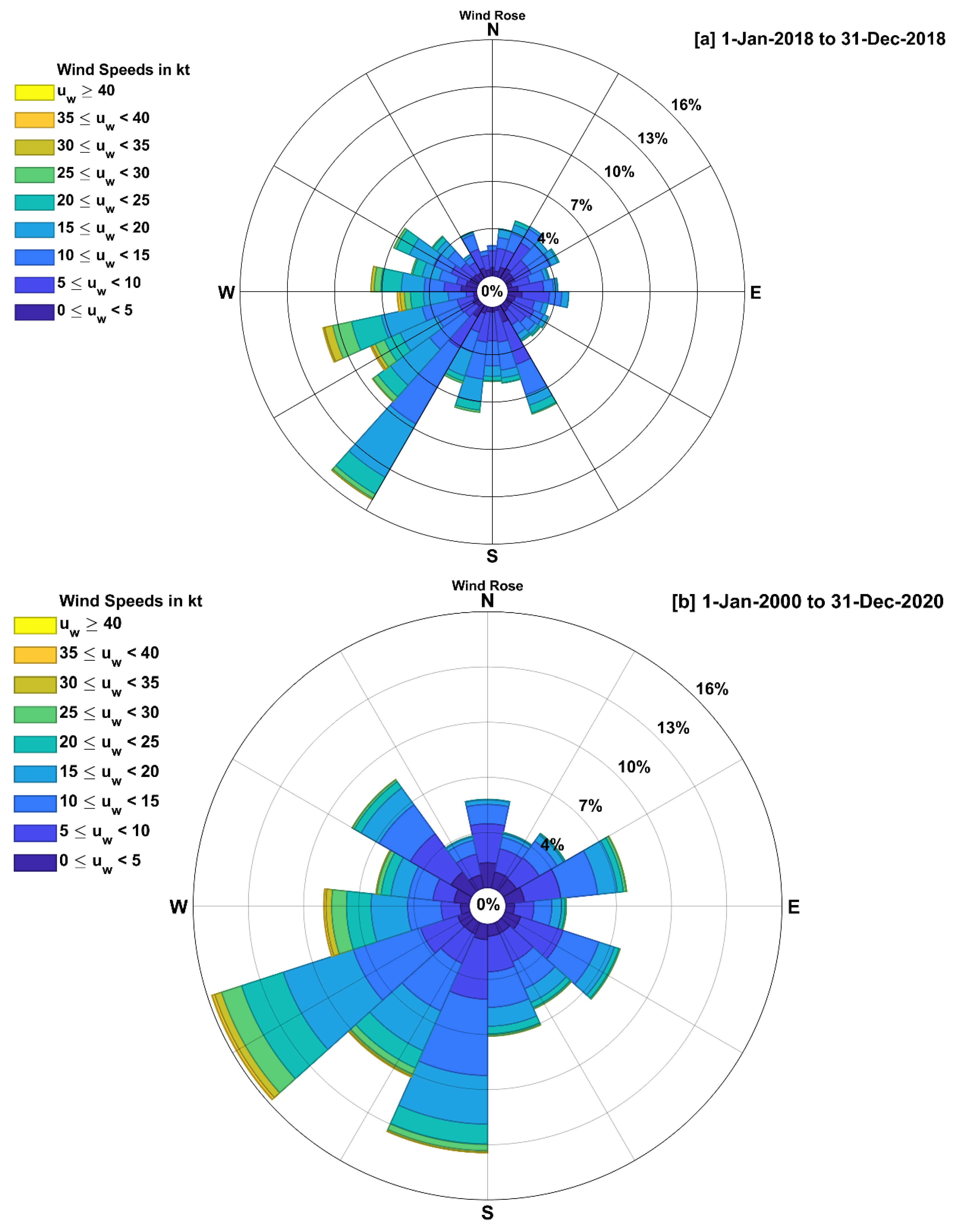
3.3. Estimation of the Net Flow through Clew Bay

One of the objectives of our study is to estimate the rate of inflow across Clew Bay and the wind speed and direction for different months using our model results from the previous section. This information is of great importance to a variety of stakeholders, especially scientists working on salmon migration. Figure 11a,b shows the average monthly water inflow through the Clew Bay cross section across the southern channel. The inflow rate is estimated from the barotropic velocity of the model times the cross-section area (i.e., depth × dy) over the line shown in Figure 1 map. The maximum water inflow (>6 × 10³ m3/s) is observed in January, while the minimum (<1 × 10³ m3/s) occurs in March 2018. There is an interesting coincidence of the maximum and minimum values of wind speed with the maximum and minimum values of inflow rate in the cross section of the bay (Figure 11a,b). The prevailing direction for all months except June and March is south-west (i.e., 270° > direction > 180°; Figure 11b). The south-westerly wind increases the inflow of water into the bay, while it is north-westerly in March (i.e. 270° > direction > 360°) and south-easterly in June (i.e. 180 > direction > 90). The water inflow rate in the bay is strongly dependent on the wind speed and direction as demonstrated by Figure 11a,b.
To get a better idea of the prevailing wind direction for the Clew Bay region, we drew the wind rose for the model in 2018 and compared it to historical wind data from 2000 to 2021 obtained from the Met Éireann Belmullet weather station (see Figure 12a,b). The predominant wind direction (>13%) from the model (2018) and the Belmullet station (2000–2020) was south-west (Figure 12a,b), confirming our earlier results in Figure 11b.

4. Conclusions

In this paper, we present for the first time a preliminary result of a high-resolution one-way nested hindcast simulation based on ROMS for the Clew Bay region. The model is driven by lateral boundary conditions taken every 10 min from the NEA _ROMS model [7] and atmospheric forcing 3-hourly ECMWF surface fields. Eight freshwater sources were specified, and a wetting and drying scheme implemented. The simulation of the Clew Bay model was validated and calibrated with available observations (e.g., ADCP, vertical salinity and temperature profiles, and tide gauges) in the geographic area of the model domain.
The correlation coefficient and RMSD between the model and ADCP temperature sensor in the inner bay were 0.99 and 0.5 °C, respectively. For the ADCP at Clare Island bottom temperature, the correlation coefficient was 0.97 and the RMSD was nearly 0.53 °C. The Taylor diagram also showed that the simulated temperature variations were close to those observed. We attribute this to the correct model forcing and the fine horizontal resolution (80 m), which helped to resolve the temperature in the model domain accurately. The Taylor diagrams for the barotropic velocity components (u, v) showed that the model for the Clare Island ADCP site was closer to the observations than the model for the inner bay ADCP. This could be due to the effect of coastal waves; this feature is not implemented in the Clew Bay model [41]. This coastal wave effect according to [42] is smaller in deep areas (i.e., Clare Island area with a depth of about 40 m), but larger in shallow areas such as the inner bay with a depth of 15 m. In addition, the highest correlation coefficients (R > 0.80) for the u component between model and ADCPs were found in Clare Island and the inner bay. The modeled meridional current velocity (v-component) in the inner bay is much weaker than the observed value, which could be the reason for the (poor) correlation (R~0.2) of the v-component values. The resemblance in structure between the model ancad the observed EPA salinity profiles indicates the correct definition of the turbulence closure parameters for the k-ε (GLS) scheme in the model.
The model density agreed with the observations at all stations, particularly in the upper 10 m, and the RMSE ranged from 0.06 to 0.23. The Clew Bay model was able to reproduce vertical profiles in the study area when compared to the EPA. Moreover, the Taylor diagram revealed that the amplitude of the simulated SSH fluctuations was similar to that observed from the Roonagh Tide Gauge Station. The model’s correlation coefficient with the tidal SSH level was 0.99 with an RMSD of 0.09 m.
There were similarities between all months in the circulation patterns of Clew Bay. Water flows into Clew Bay south of Clare Island, while north of Clare Island we see an outflow with a cyclonic motion inside the bay. The current south and north of Clare Island into and out of Clew Bay was stronger in winter. The northward flow north of Clare Island was bounded in winter and summer 2018 by the extent of a small cyclonic circulation region near 53°51′ N and 10°00′ W.
The maximum water inflow (>6 × 10³ m3/s) was found in January, while the minimum (<1 × 10³ m3/s) occurred in March 2018. We noticed a match between the maximum and minimum values of wind speed and the maximum and minimum values of inflow rate. During the winter of 2018, when a strong south-west wind predominated, the inflow of water into the bay was at its highest. The bay’s water inflow rate was highly influenced by the wind’s velocity and direction.

Author Contributions

Conceptualization, H.N., I.M., G.N., R.W. and T.D.; methodology, H.N. and I.M.; validation, H.N., I.M., G.N., R.W. and T.D.; formal analysis, H.N., I.M., G.N., R.W. and T.D., investigation, H.N., I.M., G.N. and T.D.; resources, H.N., I.M., G.N., R.W. and T.D.; data curation, H.N., I.M., G.N., R.W. and T.D.; writing—original draft preparation, H.N., G.N., R.W. and T.D.; writing—review and editing G.N., R.W. and T.D.; visualization, H.N., I.M., G.N., R.W. and T.D.; supervision, G.N., R.W. and T.D.; project administration, G.N. and T.D.; funding acquisition, INTERREG Atlantic Area Cross-border Cooperation Programme project “Innovation in the Framework of the Atlantic Deep Ocean” (iFADO, under contract EAPA 165/2016. All authors have read and agreed to the published version of the manuscript.

Funding

The validation of the model was funded by the INTERREG Atlantic Area Cross-border Cooperation Programme project “Innovation in the Framework of the Atlantic Deep Ocean” (iFADO, under contract EAPA 165/2016).

Institutional Review Board Statement

Not applicable.

Informed Consent Statement

Not applicable.

Data Availability Statement

The original contributions presented in the study are included in the article, further inquiries can be directed to the corresponding author.

Acknowledgments

The authors are grateful to INTERREG Atlantic Area Cross-border Cooperation Programme project “Innovation in the Framework of the Atlantic Deep Ocean” (iFADO, under contract EAPA 165/2016) for supporting this study. We would like to thank Kieran Lyons for preparing ADCPs data that used in the Clew Bay validation. Thanks also to Georgina McDermott and John Keogh for the collection and validation of the EPA monitoring data. Thanks to the Irish Meteorological Service (Met Éireann) for providing historical wind data from Belmullet station (https://www.met.ie/climate/available-data/historical-data, accessed on 31 January 2023). Many thanks to the three anonymous reviewers for their insightful and constructive comments on the manuscript.

Conflicts of Interest

The authors declare no conflict of interest.

References

  1. Dúchas, E.P. A Survey of Selected Littoral and Sublittoral Sites in Clew Bay, Co.Mayo; A report prepared by Aqua-Fact International Ltd for Dúchas, Department of Arts Heritage and the Gaeltacht; Aqua-Fact International Limited: Galway, Ireland, 1999; p. 33. [Google Scholar]
  2. Hiscock, K. In situ survey of subtidal (epibiota) biotopes using abundance scales and check lists at exact locations (ACE surveys). In Biological Monitoring of Marine Special Areas of Conservation: A Handbook of Methods for Detecting Change Part 2. Procedural Guidelines; Hiscock, K., Ed.; Joint Nature Conservation Committee: Peterborough, UK, 1998; Version 1 of 23. [Google Scholar]
  3. De Grave, S.; Fazakerley, H.; Kelly, L.; Guiry, M.D.; Ryan, M.; Walshe, J. A Study of Selected Maërl Beds in Irish Waters and their Potential for Sustainable Extraction. In Marine Resource Series 10; Marine Institute: Oranmore, Galway, 2000. [Google Scholar]
  4. NPWS. Clew Bay Complex, (SAC Site Code: 1482). Report in National Parks and Wildlife Service, Conservation Objectives Supporting Document Marine Habitats and Species; NPWS: Dublin, Ireland, 2011; p. 2. [Google Scholar]
  5. Annual Aquaculture Report. A Snapshot of Ireland’s Aquaculture Sector. Statistics on Production, Price and Employment in the Primary Aquaculture Sector in 2022 Based on Our Annual National Seafood Survey of All Licensed Aquaculture Producers; BIM—Seafood Development Agency: Dublin, Ireland, 2022; pp. 49–54. Available online: https://bim.ie/publications/aquaculture (accessed on 23 December 2022).
  6. BIM. The Economic Contribution of the Aquaculture Sector Across Ireland’s Bay Areas. Collective Bay Report. The Economic Impact of the Aquaculture Sector Clew Bay; BIM—Seafood Development Agency: Dublin, Ireland, 2022; p. 10. Available online: https://bim.ie/wp-content/uploads/2022/05/Clew-Bay-Report-SPREADS.pdf (accessed on 23 December 2022).
  7. Nagy, H.; Lyons, K.; Nolan, G.; Cure, M.; Dabrowski, T. A Regional Operational Model for the North East Atlantic: Model Configuration and Validation. J. Mar. Sci. Eng. 2020, 8, 673. [Google Scholar] [CrossRef]
  8. Nagy, H.; Pereiro, D.; Yamanaka, T.; Cusack, C.; Nolan, G.; Tinker, J.; Dabrowski, T. The Irish Atlantic CoCliME case study configuration, validation and application of a downscaled ROMS ocean climate model off SW Ireland. Harmful Algae 2021, 107, 102053. [Google Scholar] [CrossRef]
  9. Dabrowski, T.; Lyons, K.; Nolan, G.; Berry, A.; Cusack, C.; Silke, J. Harmful algal bloom forecast system for SW Ireland. Part I: Description and validation of an operational forecasting model. Harmful Algae 2016, 53, 64–76. [Google Scholar] [CrossRef]
  10. Cure, M.; Lyons, K.; Nolan, G. Operational Forecasting in the IBIROOS Region. In Proceedings of the Adjoint Modeling and Applications, San Diego, CA, USA, 24–26 October 2005. [Google Scholar]
  11. Elliott, A.; Hartnett, M.; O’Riain, G.; Dollard, B. The PRISM Project: Predictive Irish Sea Models. Final Report; Catchment to Coast Research Centre University of Wales Aberystwyth and Bangor Ceredigion: Aberystwyth, UK, 2007. [Google Scholar]
  12. Olbert, A.I.; Dabrowski, T.; Nash, S.; Hartnett, M. Regional modelling of the 21st century climate changes in the Irish Sea. Cont. Shelf Res. 2012, 41, 48–60. [Google Scholar] [CrossRef]
  13. Wen, L. Three-Dimensional Hydrodynamic Modelling in Galway Bay. Ph.D. Thesis, University College Galway, Galway, Ireland, 1995. [Google Scholar]
  14. Ren, L.; Nash, S.; Hartnett, M. Observation and modeling of tide- and wind-induced surface currents in Galway Bay. Water Sci. Eng. 2015, 8, 345–352. [Google Scholar] [CrossRef]
  15. Ren, L.; Nagle, D.; Hartnett, M.; Nash, S. The Effect of Wind Forcing on Modeling Coastal Circulation at a Marine Renewable Test Site. Energies 2017, 10, 2114. [Google Scholar] [CrossRef]
  16. Ren, L.; Miao, J.; Li, Y.; Luo, X.; Li, J.; Hartnett, M. Estimation of Coastal Currents Using a Soft Computing Method: A Case Study in Galway Bay, Ireland. J. Mar. Sci. Eng. 2019, 7, 157. [Google Scholar] [CrossRef]
  17. Nagy, H.; Lyons, K.; Dabrowski, T. A Regional Operational and Storm Surge Model for the Galway Bay: Model Configuration and Validation. In Proceedings of the Ocean Sciences Meeting, San Diego, CA, USA, 16–21 February 2020. [Google Scholar] [CrossRef]
  18. Calvino, C.; Dabrowski, T.; Dias, F. A study of the sea level and current effects on the sea state in Galway Bay, using the numerical model COAWST. Ocean Dyn. 2022, 72, 761–774. [Google Scholar] [CrossRef]
  19. Calvino, C.; Dabrowski, T.; Dias, F. Current interaction in large-scale wave models with an application to Ireland. Cont. Shelf Res. 2022, 245, 104798. [Google Scholar] [CrossRef]
  20. Mamotous, I.; Dabrowki, T.; Lyons, K.; McCoy. A two way nested high resolution coastal simulation in a tidally dominated area: Preliminary results. In Proceedings of the 8th EuroGOOS Conference, Bergen, Norway, 3–5 October 2017. [Google Scholar]
  21. Shchepetkin, A.F.; McWilliams, J.C. The Regional Ocean Modeling System (ROMS): A split-explicit, free-surface, opography following coordinates ocean model. Ocean Model. 2005, 9, 347–404. [Google Scholar] [CrossRef]
  22. Wilkin, J.; Zhang, W.G.; Cahill, B.; Chant, R.C. Integrating coastal models and observations for studies of ocean dynamics, observing systems and forecasting. In Operational Oceanography in the Ocean forecasting in the 21st Century; Schiller, A., Brassington, G., Eds.; Springer: Dordrecht, The Netherlands, 2011; pp. 487–512. [Google Scholar]
  23. Sikirić, M.D.; Janekovic, L.; Kuzmic, M. A new approach to bathymetry smoothing is sigma coordinate ocean models. Ocean. Model. 2009, 29, 128–136. [Google Scholar] [CrossRef]
  24. Haney, R.L. On the pressure gradient force over steep bathymetry in sigma coordinates ocean models. Phys. Oceanogr. 1991, 21, 610–619. [Google Scholar] [CrossRef]
  25. Shapiro, R. Linear filtering. Math. Comput. 1975, 29, 1094–1097. [Google Scholar] [CrossRef]
  26. Warner, J.C.; Defne, Z.; Haas, K.; Arango, H.G. A wetting and drying scheme for ROMS. Comput. Geosci. 2013, 58, 54–61. [Google Scholar] [CrossRef]
  27. O’Dea, E.; Bell, M.J.; Coward, A.; Holt, J. Implementation and assessment of a flux limiter based wetting and drying scheme in NEMO. Ocean Model. 2020, 155, 101708. [Google Scholar] [CrossRef]
  28. Umlauf, L.; Burchard, H. A generic length-scale equation for geophysical turbulence models. J. Mar. Res. 2003, 61, 235–265. [Google Scholar] [CrossRef]
  29. Warner, J.C.; Sherwood, C.R.; Arango, H.G.; Signell, R.P. Performance of four turbulence closure models implemented using a generic length scale method. Ocean Model. 2005, 8, 81–113. [Google Scholar] [CrossRef]
  30. Shchepetkin, A.F.; McWilliams, J.C. Quasi-Monotone Advection Schemes Based on Explicit Locally Adaptive Dissipation. Mon. Weather Rev. 1998, 126, 1541–1580. [Google Scholar] [CrossRef]
  31. Smolarkiewicz, P.K.; Margolin, L.G. MPDATA: A Finite-Difference Solver for Geophysical Flows. J. Comput. Phys. 1998, 140, 459–480. [Google Scholar] [CrossRef] [Green Version]
  32. Arheimer, B.; Wallman, P.; Donnelly, C.; Nyström, K.; Pers, C. E-HypeWeb: Service for Water and Climate Information—And Future Hydrological Collaboration across Europe? In Environmental Software Systems. Frameworks of EEnvironment, Proceedings of the 9th IFIP WG 5.11 International Symposium, ISESS 2011, Brno, Czech Republic, 27–29 June 2011; Hřebíček, J., Schimak, G., Denzer, R., Eds.; Springer: Berlin/Heidelberg, Germany, 2011; Volume 359, pp. 657–666. [Google Scholar] [CrossRef]
  33. Joseph, A. Chapter 11—Vertical Profiling of Currents Using Acoustic Doppler Current Profilers. In Measuring Ocean Currents; Elsevier: Amsterdam, The Netherlands, 2014; pp. 339–379. [Google Scholar] [CrossRef]
  34. Fischer, J.; Visbeck, M. Deep Velocity Profiling with Self-contained ADCPs. J. Atmos. Ocean. Technol. 1993, 10, 764–773. [Google Scholar] [CrossRef]
  35. Comas-Rodríguez, I.; Hernández-Guerra, A.; McDonagh, E. Referencing geostrophic velocities using ADCP data Referencing geostrophic velocities using ADCP data. Sci. Mar. 2010, 74, 331–338. [Google Scholar] [CrossRef]
  36. Kim, D.; Yu, K. Uncertainty estimation of the ADCP velocity measurements from the moving vessel method, (I) development of the framework. KSCE J. Civ. Eng. 2010, 14, 797–801. [Google Scholar] [CrossRef]
  37. Pawlowicz, R.; Beardsley, B.; Lentz, S. Classical tidal harmonic analysis including error estimates in MATLAB using T_TIDE. Comput. Geosci. 2002, 28, 929–937. [Google Scholar] [CrossRef]
  38. Pereira, D. Wind Rose, MATLAB Central File Exchange 2023. Available online: https://www.mathworks.com/matlabcentral/fileexchange/47248-wind-rose (accessed on 31 January 2023).
  39. Taylor, K.E. Summarizing multiple aspects of model performance in a single diagram. J. Geophys. Res. Atmos. 2001, 106, 7183–7192. [Google Scholar] [CrossRef]
  40. Bernsen, E.; Dijkstra, H.A.; Wubs, F. A method to reduce the spin-up time of ocean models. Ocean Model. 2008, 20, 380–392. [Google Scholar] [CrossRef]
  41. Hordoir, R.; Axell, L.; Höglund, A.; Dieterich, C.; Fransner, F.; Gröger, M.; Liu, Y.; Pemberton, P.; Schimanke, S.; Andersson, H.; et al. Nemo-Nordic 1.0: A NEMO-based ocean model for the Baltic and North seas—Research and operational applications. Geosci. Model Dev. 2019, 12, 363–386. [Google Scholar] [CrossRef]
  42. Aijaz, S.; Ghantous, M.; Babanin, A.V.; Ginis, I.; Thomas, B.; Wake, G. Nonbreaking wave-induced mixing in upper ocean during tropical cyclones using coupled hurricane-ocean-wave modeling. J. Geophys. Res. Oceans 2017, 122, 3939–3963. [Google Scholar] [CrossRef] [Green Version]
  43. Dias, J.; Lopes, J. Implementation and assessment of hydrodynamic, salt and heat transport models: The case of Ria de Aveiro Lagoon (Portugal). Environ. Model. Softw. 2006, 21, 1–15. [Google Scholar] [CrossRef]
  44. Lopes, J.F. Using Different Classic Turbulence Closure Models to Assess Salt and Temperature Modelling in a Lagunar System: A Sensitivity Study. J. Mar. Sci. Eng. 2022, 10, 1750. [Google Scholar] [CrossRef]
  45. Nagy, H.; Elgindy, A.; Pinardi, N.; Zavatarelli, M.; Oddo, P. A nested pre-operational model for the Egyptian shelf zone: Model configuration and validation/calibration. Dyn. Atmos. Oceans 2017, 80, 75–96. [Google Scholar] [CrossRef]
  46. Mungall, J.; Matthews, J. The M2 tide of the Irish Sea: Hourly configurations of the sea surface and of the depth-mean currents. Estuar. Coast. Mar. Sci. 1978, 6, 55–74. [Google Scholar] [CrossRef]
  47. Robinson, I.S. The tidal dynamics of the Irish and Celtic Seas. Geophys. J. Int. 1979, 56, 159–197. [Google Scholar] [CrossRef]
  48. O’Rourke, F.; Boyle, F.; Reynolds, A. Tidal energy update. Appl. Energy 2009, 87, 398–409. [Google Scholar] [CrossRef]
  49. O’Rourke, F.; Boyle, F.; Reynolds, A. Tidal current energy resource assessment in Ireland: Current status and future update. Renew. Sustain. Energy Rev. 2010, 14, 3206–3212. [Google Scholar] [CrossRef]
  50. Flather, R.A.; Williams, J.A. Climate change effects on the storm surge: Methodologies and results. In Climate Scenarios for Water-Related and Coastal Impact; ECLAT-2 Workshop Report; Beersma, J., Agnew, M., Viner, D., Hulme, M., Eds.; CRU: Norwich, UK, 2000; pp. 66–78. [Google Scholar]
  51. Taniguchi, N.; Huang, C.; Arai, M.; Howe, B.M. Variation of Residual Current in the Seto Inland Sea Driven by Sea Level Difference Between the Bungo and Kii Channels. J. Geophys. Res. Oceans 2018, 123, 2921–2933. [Google Scholar] [CrossRef]
  52. Proctor, R. Tides and Residual Circulation in the Irish Sea: A Numerical Modelling Approach. Ph.D. Thesis, University of Liverpool, Liverpool, UK, 1981. Available online: https://ethos.bl.uk/OrderDetails.do?uin=uk.bl.ethos.378225 (accessed on 14 November 2022).
Figure 1. Bathymetric map of the area covered by the model. The major rivers included in the model are indicated by red circles. Two ADCPs, four observed vertical temperature and salinity profiles (CW030, CW110, CW130, and CW140) by the Environmental Protection Agency (EPA) in Ireland, and tide gauge locations are indicated by black circles. Monthly average net flow values in [m3/s] were obtained for the cross section shown on the map by a solid black line.
Jmse 11 00362 g001
Figure 2. Temporal comparison between the Clew Bay model (in continuous red lines) and observed (in continuous blue lines) bottom temperature in [°C] for the period from 25 July to 20 December 2017 for (a) Inner Bay (b) Clare Island.
Jmse 11 00362 g002
Figure 3. Taylor diagram assessing the Clew Bay model (red solid circle) and observed temperature (black solid circle) [°C] in terms of correlation, STD in [°C], and RMSD in [°C] for (a) Model Inner Bay, and (b) Model Clare Island.
Jmse 11 00362 g003
Figure 4. Taylor diagrams assessing the barotropic velocity components for ADCPs (black solid circle) and the Clew Bay model (red solid circle) for Inner Bay and Clare Island. In terms of correlation, STD in [m/s] and RMSD in [m/s] are shown for the period from 25 July to 20 December 2017, for (a,b) East barotropic velocity component (u) and (c,d) North barotropic velocity component (v).
Jmse 11 00362 g004
Figure 5. Current rose for ADCPs in black continuous line and the Clew Bay model in red continuous line, showing the distribution of current direction from 25 July to 20 December 2017, for (a,b) Inner Bay and (c,d) Clare Island.
Jmse 11 00362 g005aJmse 11 00362 g005b
Figure 6. Vertical profiles of modeled (continuous red lines) temperature, salinity, and density and observations (continuous blue lines) for different EPA stations on 20 September 2017. The EPA stations are, from top to bottom, (a) CW030, (b) CW110, (c) CW130, and (d) CW140. The maps show the EPA stations’ location.
Jmse 11 00362 g006aJmse 11 00362 g006b
Figure 7. Taylor diagram assessing the sea surface height (SSH) representation, in terms of correlation, STD and RMSD in meters, produced by the Clew Bay Model and Roonagh tide gauge station sea surface height (SSH) [meters]. The diagram is based on the period from 14 August 2017 to 2 January 2018 on 6 min frequency showing observations of the tide gauge (black solid circle) and model (red solid circle).
Jmse 11 00362 g007
Figure 8. Clew Bay Model and Roonagh Tide Gauge Station surges [meters]. The temporal evolution based on the period from 14 August 2017 to 2 January 2018 on 6 min frequency showing tide gauge surge (black continuous line) and model (green continuous line). Storm surges are denoted by the letters A, B, C, and D.
Jmse 11 00362 g008
Figure 9. Monthly averaged barotropic velocity [m/s] fields (speed and direction denoted by arrows) for (a) January and (b) July.
Jmse 11 00362 g009
Figure 10. Residual barotropic velocity [m/s] fields (speed and direction denoted by vectors or arrows) showing (a) spring tide averaged over 10 September 2018 and (b) neap tide averaged over 2 October 2018.
Jmse 11 00362 g010
Figure 11. (a) The monthly average values of inflow in [m3/s] over the cross section shown on the Figure 1 map, and (b) The monthly average values of wind speed [m/s].
Jmse 11 00362 g011
Figure 12. Wind rose for (a) Clew Bay model in from 1 January to 31 December 2018, and (b) Met Éireann Belmullet station from 1 January 2000 to 31 December 2020, showing the distribution of wind direction and wind speed in knots.
Jmse 11 00362 g012
Table 1. The Clew Bay model turbulence closure parameters for the GLS scheme.
Parameter DefinitionValue
GLS_PStability exponent (non-dimensional)3.0
GLS_MTurbulent kinetic energy exponent (non-dimensional).1.5
GLS_NTurbulent length scale exponent (non-dimensional)−1.0
GLS_KminMinimum value of specific turbulent kinetic energy7.6 × 10−6
GLS_PminMinimum value of dissipation1.0 × 10−12
GLS_CMU0Stability coefficient0.5477
GLS_C1Shear production coefficient1.44
GLS_C2Dissipation coefficient1.92
GLS_C3MBuoyancy production coefficient (minus)−0.4
GLS_C3PBuoyancy production coefficient (plus)1.0
GLS_SIGKConstant Schmidt number (non-dimensional)
for turbulent kinetic energy diffusivity
1.0
GLS_SIGPConstant Schmidt number (non-dimensional)
for turbulent generic statistical field
1.3
Table 2. Mean annual freshwater discharge values [m3/s] in the Clew Bay model.
RegionRiver NameMean Annual Discharge
[m3/s]
Clew BayOwenwee7.61
Newport5.54
Bunowen3.17
Owengrave2.49
Mayour1.99
Westport1.64
Owennabrockagh1.98
Burrishoole Abbey 4.98
Table 3. The EPA station locations for temperature and salinity profiles in latitude and longitude (in degrees) sampled on 20 September 2017.
Station NameLatitude °NLongitude °W
CW03053.8237229.66330600000
CW11053.8493509.71932597800
CW13053.8379839.78848080500
CW14053.7960009.77628176973
Table 4. The amplitudes in meters and phases in degrees for six of the principal tidal constituents calculated, for the measured and modeled data, with the differences (model–tide gauge) between them for the period from 14 August 2017 to 2 January 2018.
Tidal (Main) ConstituentsModel
Amplitude
T.G Amplitude DifferenceModel
(Phase Angle)
T.G
(Phase Angle)
Difference
M21.3601.310+0.050180.22180.65−0.43
S20.5090.508+0.001212.62210.28+2.34
N20.2780.263+0.015158.72161.72−3.00
K10.1360.135+0.001105.2796.08+9.19
O10.0730.078−0.005329.97333.08−3.11
Q10.0110.0110.000299.23301.01−1.78
Disclaimer/Publisher’s Note: The statements, opinions and data contained in all publications are solely those of the individual author(s) and contributor(s) and not of MDPI and/or the editor(s). MDPI and/or the editor(s) disclaim responsibility for any injury to people or property resulting from any ideas, methods, instructions or products referred to in the content.

