Quantized Sliding Mode Fault-Tolerant Control for Unmanned Marine Vehicles with Thruster Saturation

Abstract

In this paper, the sliding mode technique is used to study the quantized fault-tolerant control of unmanned marine vehicles with thruster saturation. Firstly, the sliding mode surface is constructed according to the full rank decomposition of input matrix, and the stability of sliding mode is guaranteed by linear matrix inequalities. An improved dynamic adjustment scheme of quantization parameter is proposed. Compared with the original adjustment scheme, the relationship between quantization parameter and desired targets is increased, so that the adjustment range of quantization parameters is more comprehensive. The sliding mode controller is combined with quantization parameter adjustment strategy to ensure the asymptotic stability of unmanned marine vehicles system. In addition, compared with the existing research results of quantitative fault tolerance problem without considering saturation, this paper gives a result of the domain of attraction affected by the fault of the thruster. Finally, the superiority of the proposed method is verified by simulation comparison.

1. Introduction

Unmanned marine vehicles (UMVs) have been widely used in different application scenarios (such as ocean rescue and deep-sea exploration, etc.) [1,2]. With the rapid development of digital communication technology, feedback control system for UMVs gradually develops turn analog control to digital control [3]. Due to the limitation of communication channel with limited bandwidth, quantization phenomenon will inevitably occur. In this case, it is necessary to process signal quantization [4]. So the quantification of the feedback control system of UMVs has always been the subject of in-depth study.

Data transmitted after rough quantization may affect robustness and even control performance [5]. To avoid performance degradation due to quantization effects, the following articles [6,7,8,9,10,11,12] address quantization phenomena. A hybrid switched fuzzy system was established considering the Denial of Service attack and quantization effect in [6]. In order to achieve the trajectory tracking control objectives, [7] structured a new quantized extended state observer and adaptive anti-jamming control laws. The quantization effect was overcome in [8] by introducing the bound of quantization error. Paper [9] proposed an adaptive backstepping sliding mode control scheme to solve the problems of dynamic uncertainty, external disturbance and quantization error. For quantization errors, a dynamic uniform quantization scheme [10] was put forward and the stability of uncertain systems with quantization was studied. The sliding mode control of a class of continuous time switching systems with signal quantization, actuator nonlinearity and persistent dwell-time switching was studied in [11]. By two quantization schemes (dynamic uniform quantization scheme and static logarithm quantization scheme), a new quantization sliding mode control method was proposed [12], which can completely compensate the quantization effect by injecting quantizer parameters into the controller gain.

Due to long-term operation in complex marine environment for UMVs, thruster failure is inevitable, and it is not feasible to repair or replace the failed thruster immediately [13], so FTC (fault-tolerant control) is necessary for UMVs system. For the problem of thruster failure, based on fuzzy control [14], SMC(sliding mode control) [15], model predictive control [16], fast terminal sliding mode control [17] and other classical control methods, a series of FTC schemes were proposed. Meanwhile, the results of simultaneous treatment of quantization and thruster failures have been published in the existing work [14,15,18,19,20,21,22]. A damping term with the estimation of unknown bounds and a positive time-varying integral function were constructed in [14] respectively to handle input quantization and actuator faults. Further, an adaptive fuzzy control scheme basedon observer was proposed. In [18], the author dealt with the adaptive fault-tolerant control problem for system with actuator faults and signal quantization effects. A method of unmanned ship system stability based on sliding mode variable structure technology [19] was proposed under network environment. To solve the actuator fault problem of T-S fuzzy system, a novel event-triggered adaptive sliding mode control stabilization scheme [20] based on quantized state vector was proposed. The problem of quantization design of sliding mode observer for a class of Markov jump systems with actuator failures was studied in [21], a new sliding mode observer method based on quantization signal was proposed, the actuator faults were suppressed by off-line static compensation of quantization effects and synthesis of discontinuous inputs. The design in [22] used the quantized state information to construct the adaptive fuzzy laws, which can completely compensate the time-varying faults and quantization errors. On the other hand, ocean disturbances may affect the normal operation of UMVs. Considering the disturbances problem, paper [23] proposed control strategy based on sliding mode technology. Based on the dynamic sliding mode control theory, the controller was designed to improve the robustness of the over-actuated autonomous underwater vehicle system under the influence of ocean currents and model uncertainties.

In practice, actuator execution of UMVs is usually rather limited, thereby, rendering excessively large control efforts cannot be feasibly executed [24]. The phenomenon of saturation is not considered in the above literatures. Once the thruster saturation phenomenon is ignored, the stability of UMVs system may be destroyed [25]. Considering the limitation of input saturation, the composite nonlinear feedback controller in [26,27] is designed appropriately. By solving the linear matrix inequality problem, the parameters of complex nonlinear feedback input are derived. Nevertheless, quantization becomes more complicated when considering thruster saturation, because quantization, thruster failure and saturation are intertwined. For linear uncertain systems, the relationship between parameters of quantification and failure have been described in [28], the existing results are no longer applicable to UMVs systems taking into satuation account. Therefore, for UMVs quantization error control problem, it is essential to deal with the interaction between thruster saturation and quantization effects and to design a quantized sliding mode fault-tolerant controller based on the UMVs model. This is the main motivations for this paper.

Based on the above discussion, this paper will study the quantitative FTC of UMVs by sliding-mode technology under ocean disturbance, thruster failure and saturation. Meanwhile, a dynamic adjustment strategy of quantitative parameters is proposed. The main contributions are as follows.

(1)

Based on the sliding mode technique, a new fault-tolerant controller is designed, which can ensure the asymptotic stability of UMVs system and compensate the effects of quantization, thruster failure and saturation.

(2)

The relationship among UMVs quantization parameter, fault information and desired target is revealed. A more comprehensive range of quantitative parameter adjustment is given. This range can be reduce to the result with neglecting desired target in [28], and further reduce to the existing result with neglecting thruster failure in [29].

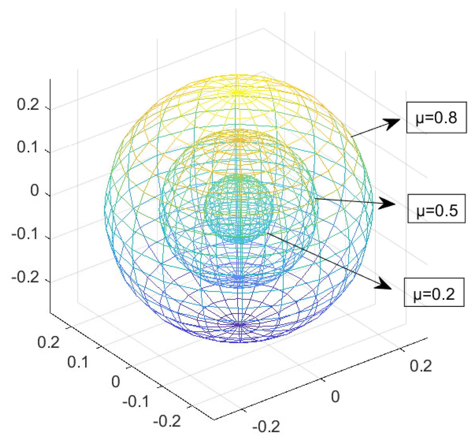
(3)

The region of attraction (sphere ${\Gamma }_0$) affected by thruster failure is described, and through the optimization parameter k solved by linear matrix inequalities (LMIs), the optimized region of attraction $\Gamma$ can be obtained.

This paper will be explained in the following sections. In Section 2, a unified and comprehensive UMV model is established. The quantization control law and the adjustment strategy of quantization parameters are presented, and the stability analysis and reachability proof of sliding mode surface are carried out in Section 3. In Section 4 and Section 5 show the simulation comparison results and conclusions respectively.

2. Problem Statement

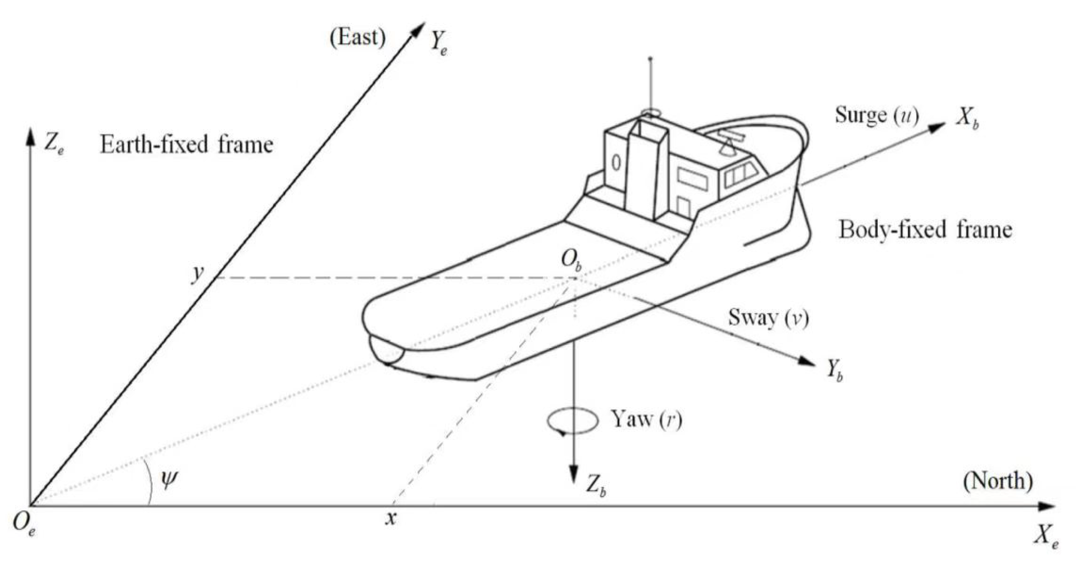
2.1. UMV Model

The kinematics and dynamics model [5] of a nonlinear anchored unmanned marine vehicle are considered in this paper. Kinematic and dynamic equations are described as

$$\dot{\eta }\left(t\right)=J\left(\psi \left(t\right)\right)v\left(t\right)$$

(1)

$$M\dot{v}\left(t\right)+Nv\left(t\right)+E\eta \left(t\right)=\Gamma u\left(t\right)$$

(2)

where $\eta \left(t\right)={\left[x_e\left(t\right),y_e\left(t\right),\psi \left(t\right)\right]}^T$ represents the position and yaw angle respectively in the earth-fixed reference frame and $v\left(t\right)={\left[u\left(t\right),\nu \left(t\right),r\left(t\right)\right]}^T$ represents surge, sway and yaw velocities respectively in the body-fixed reference frame for UMV. Figure 1 is the UMV system in the reference coordinate system. M, N, and E represent the matrix of inertia, damping, and mooring forces respectively. $u\left(t\right)$ is the thruster forces vector, $\Gamma$ is a configuration matrix. And $J\left(\psi \left(t\right)\right)=\left[\begin{array}{ccc}cos\left(\psi \left(t\right)\right)& -sin\left(\psi \left(t\right)\right)& 0\\ sin\left(\psi \left(t\right)\right)& cos\left(\psi \left(t\right)\right)& 0\\ 0& 0& 1\end{array}\right]$. As mentioned in [30], for dynamic positioning vessel on mission, the speed of rotation around the vertical direction of the earth is always slow. Hence, $\psi \left(t\right)\approx 0$ and $J\left(\psi \left(t\right)\right)\approx I$ would be obtained through $\psi \left(t\right)$ is small enough.

The thruster fault model [15] that includs total fault, partial fault and stuck fault, the form is as follows

$$u_{ij}^F\left(t\right)={\rho }_i^j{u}_i\left(t\right)+{\sigma }_i^j{u}_{si}\left(t\right)$$

(3)

where $i=1,\dots m$, $j=1,\dots l$ and l is the number of total fault modes. For the ith thruster in the jth fault mode, $u_{ij}^F,u_i\left(t\right),u_{si}\left(t\right)$ denote thruster force, thruster commands and thruster unknown time-varying bounded dead-stuck fault, respectively. ${\rho }_i^j,{\sigma }_i^j$ are thruster effectiveness coefficient and stuck fault coefficient. Then, the following matrices are introduced:

$$\begin{array}{cc}\hfill & {\rho }^j=diag\left\{{\rho }_1^j,{\rho }_2^j,\dots ,{\rho }_m^j\right\},{\rho }_i^j\in \left[{\underline{\rho }}_i^j,{\overline{\rho }}_i^j\right]\hfill \\ & {\sigma }^j=diag\left\{{\sigma }_1^j,{\sigma }_2^j,\dots ,{\sigma }_m^j\right\},{\sigma }_i^j=0or1\hfill \end{array}$$

where $0\le {\underline{\rho }}_i^j\le {\overline{\rho }}_i^j\le 1$. The integration of (3) is $u^F\left(t\right)=\rho u\left(t\right)+\sigma u_s\left(t\right)$, where $\rho \in {\rho }^j,\sigma \in {\sigma }^j$ and $∥u_s\left(t\right)∥\le {\overline{u}}_s$. To compensate for saturation, introducing saturation model of [31], it follows that

$$u^S\left(t\right)=sat\left(\rho u\left(t\right)+\sigma u_s\left(t\right)\right)=\rho \chi u\left(t\right)+\sigma u_s\left(t\right)$$

(4)

where sat(.) is the saturation function, $\chi \in (0,1]$ is saturation coefficient.

So, Substituting (4) into (2), the UMV model is extended as

$$\dot{v}\left(t\right)=-M^{-1}Nv\left(t\right)+M^{-1}\Gamma u^S\left(t\right)-M^{-1}E\eta \left(t\right)+\omega \left(t\right)$$

(5)

where $\omega \left(t\right)$ is the external disturbance, due to the ocean disturbances are continuously bounded, then ${\left|\omega \left(t\right)\right|}_2\le \overline{\omega }\left(t\right)$.

Define the error $e\left(t\right)=\left[\begin{array}{c}{e}_{\eta }\left(t\right)\\ e_v\left(t\right)\end{array}\right]=\left[\begin{array}{c}\eta \left(t\right)-{\eta }_{ref}\\ v\left(t\right)-v_{ref}\end{array}\right]$, ${\eta }_{ref}$ is the desired position vector, $v_{ref}$ is the desired velocity vector and $x={\left[\begin{array}{cc}{\eta }^T\left(t\right)& v^T\left(t\right)\end{array}\right]}^T$, $e_d={\left[\begin{array}{cc}{\eta }_{ref}^T& v_{ref}^T\end{array}\right]}^T$. Combining (1) and (5), we have

$$\dot{e}\left(t\right)=Ae\left(t\right)+B{u}^S\left(t\right)+B_1\omega +A{e}_d$$

(6)

where $A=\left[\begin{array}{cc}0& I\\ -M^{-1}E& -M^{-1}N\end{array}\right]$, $B=\left[\begin{array}{c}0\\ M^{-1}\Gamma \end{array}\right]$, $B_1=\left[\begin{array}{c}0\\ I\end{array}\right]$.

Denote $D=B_1\omega +A{e}_d$, then (6) becomes

$$\dot{e}\left(t\right)=Ae\left(t\right)+B{u}^S\left(t\right)+D$$

(7)

For the sake of controlling the error of yaw angle $\psi \left(t\right)$ and its velocity $r\left(t\right)$, $z\left(t\right)$ is described as

$$z\left(t\right)=Ce\left(t\right).$$

where $z\left(t\right)$ is controlled output, C is a constant matrix.

2.2. Quantizer Model

A quantitative model of the UMVs system will be presented in the following. Since the thrusters are commanded by a land-based control station, transmitted signals from input and output controllers are quantized [5]. The controller design using the following form of quantization [32] in this paper

$$Q_h\left(\varsigma \right)=hQ\left(\frac{\varsigma }{h}\right)=hround\left(\frac{\varsigma }{h}\right),h>0$$

where h is the quantization level and round(.) is the function of taking the nearest integer. Denote $e_h=Q_h\left(\varsigma \right)-\varsigma$, which need to satisfy the following conditions

$$\begin{array}{cc}\hfill & \left|e_{h_1}\right|=\left|Q_{h_1}\left(u_0\right)-u_0\right|\le {\Delta }_1{h}_1\hfill \\ & \left|e_{h_2}\right|=\left|Q_{h_2}\left(e\right)-e\right|\le {\Delta }_2{h}_2\hfill \end{array}$$

(8)

where $Q_{h_1}\left(u_0\right),Q_{h_2}\left(e\right)$ are static quantizer and dynamic quantizer respectively.

Remark 1. 

This is the first time that quantization and thruster saturation have been taken into account in fault-tolerant control of a UMV system. In the uplink channel, a static quantizer has been used to quantify the control input $u_0\left(t\right)$, and the output quantization signal is $u\left(t\right)$. In the downlink channel, a dynamic quantizer with quantization parameter $h_2$ is used to quantify the state signal $e\left(t\right)$. Under the SMC laws and the adjustment of the dynamic quantization parameter, the state of the system will reach the desired sliding mode surface and further approach the origin.

Assumption 1. 

For every $\rho \in {\rho }^j$, $j\in I(1,l)$, $rank\left(B\rho \right)=rank\left(B\right)$.

Assumption 2. 

Up to $m-n(1\le n\le m-n)$ thrusters fails, the left thrusters can complete the control objective.

2.3. Design Objectives

The purpose is by designing sliding mode fault-tolerant controller and adjustment strategy of quantization parameter to reduce oscillation of the yaw angle and its velocity in this paper.

Then The main results will be laid out in the next section.

3. Main Results

  Figure 2 is a block diagram of the UMVs system based on quantization form considering thruster failure, thruster saturation and external disturbances. Sliding mode control [15,33,34,35] as an effective tool for robustness, it not only has good robustness to external disturbance, but also has fast response ability. Therefore, sliding mode controller is selected in this paper.

3.1. Stability Analysis

Take the full rank decomposition of the matrix B:

$$B=B_{\upsilon }^{*}{N}^{*}$$

(9)

where $B\in R^{6*6}$, $B_{\upsilon }^{*}\in R^{6*3}$, $N^{*}\in R^{3*6}$. To design a controller with certain flexibility, introduce the parameter $\iota >0$ such that $B_{\upsilon }=\frac{1}{\iota }{B}_{\upsilon }^{*}$, $N=\iota N^{*}$.

The sliding mode surface $\alpha \left(e\right)$ is designed as follows

$$\alpha \left(e\right)=Se\left(t\right)=B_{\upsilon }^T{X}^{-1}e\left(t\right)=0$$

(10)

where S should meet the necessary conditions that $S{B}_v$ is nonsingular symmetric matrix and the reduced-order equivalent system is asymptotically stable; X is a positive definite matrix to be designed, which will be given in theorem 1. The stability of sliding motion is verified in the following.

Theorem 1. 

The sliding surface is given by (10). Assume $\widetilde{B_v}$ is any basis of the null space of $B_v^T$, if there are positive matrix X, matrix $K\in R^{6*3}$, parameter k and positive scalar $\gamma >0$ that are satisfied with the linear matrix inequality (11) in the following, the reduced-order system on the sliding surface is asymptotically stable and the $H_{\infty }$ performance bound is no larger than γ.

$$\left[\begin{array}{ccc}AX+X{A}^T-K{B}_{\upsilon }^T-B_{\upsilon }{K}^T& X{C}^T& I\\ *& -I& 0\\ *& *& -{\gamma }^{-2}I\end{array}\right]<0$$

(11)

$$\left[\begin{array}{cc}X& K\\ *& I\end{array}\right]>0,\left[\begin{array}{cc}X& I\\ *& kI\end{array}\right]>0$$

(12)

Proof. 

Firstly, give the following nonsingular transformation matrix M and vector v

$$M=\left[\begin{array}{c}\widetilde{B_v^T}\\ B_v^T{X}^{-1}\end{array}\right],v=\left[\begin{array}{c}{v}_1\\ v_2\end{array}\right]=Me$$

Notice that $\dot{v}=M\dot{e}=MA{M}^{-1}v+MB{u}^S\left(t\right)+MD$. Then,

$$\begin{array}{c}\hfill \dot{v}=\left[\begin{array}{cc}{A}_1& A_2\\ A_3& A_4\end{array}\right]\left[\begin{array}{c}{v}_1\\ v_2\end{array}\right]+\left[\begin{array}{c}0\\ SB\end{array}\right]u^S\left(t\right)+\left[\begin{array}{c}\widetilde{B_v^T}\\ S\end{array}\right]D\end{array}$$

where $A_1=\widetilde{B_v^T}AX\widetilde{B_{\upsilon }}{\left(\widetilde{B_v^T}X\widetilde{B_{\upsilon }}\right)}^{-1}$, $A_2=\widetilde{B_v^T}A{B}_{\upsilon }{\left(SB\upsilon \right)}^{-1}$, $A_3=SAX\widetilde{B_{\upsilon }}{\left(\widetilde{B_v^T}X\widetilde{B_{\upsilon }}\right)}^{-1}$, $A_4=SA{B}_{\upsilon }{\left(SB\upsilon \right)}^{-1}$. The reduced-order system is given by

$$\begin{array}{c}\hfill {\dot{v}}_1=A_1{v}_1+\widetilde{B_v^T}D\end{array}$$

(13)

Define $V_0=v_1^T{X}_0^{-1}{v}_1$, one has

$$\begin{array}{c}\hfill \dot{V_0}=v_1^T(X_0^{-1}{A}_1+A_1^T{X}_0^{-1})v_1+2v_1^T{X}_0^{-1}\widetilde{B_v^T}D\end{array}$$

next,

$$\begin{array}{c}\hfill \dot{V}=\dot{V_0}+z^{T}z-{\gamma }^2{D}^{T}D\le v_1^T{X}_0^{-1}{\rm Y}{X}_0^{-1}{v}_1\end{array}$$

where ${\rm Y}=A_1{X}_0+X_0{A}_1^T+{\gamma }^{-2}\widetilde{B_v^T}\widetilde{B_{\upsilon }}+X_0{\left(\widetilde{B_v^T}X\widetilde{B_{\upsilon }}\right)}^{-1}\widetilde{B_v^T}X{C}^{T}CX\widetilde{B_{\upsilon }}{\left(\widetilde{B_v^T}X\widetilde{B_{\upsilon }}\right)}^{-1}{X}_0$. Let $X_0=\widetilde{B_v^T}X\widetilde{B_{\upsilon }}$, if the following inequality can be obtained

$$\begin{array}{c}\hfill {\rm Y}=\widetilde{B_v^T}(AX+X{A}^T+{\gamma }^{-2}I+X{C}^{T}CX)\widetilde{B_{\upsilon }}<0\end{array}$$

(14)

Referring to the projection lemma, one can show that (13) is feasible if and only if the following LMI is feasible:

$$\begin{array}{c}\hfill AX+X{A}^T-K{B}_{\upsilon }^T-B_{\upsilon }{K}^T+{\gamma }^{-2}I+X{C}^{T}CX<0\end{array}$$

(15)

According to Finsler’s lemma [36], for some parameter $k_0>0$ and ${\gamma }_0$, there must be a positive definite matrix $X_0>0$, we can get

$$\begin{array}{cc}\hfill & A{X}_0+X_{0}A+{\gamma }^{-2}I+X{C}^{T}CX-2{\gamma }_0{B}_v{B}_v^T<0\hfill \\ & X_0>\frac{1}{k_0}I>0.\hfill \end{array}$$

(16)

To continue the inference, the parameter $\beta$ is introduced. There exists a positive scalar $\beta$ which satisfies ${\lambda }_{min}\left(X_0\right)/{\lambda }_{max}\left(B_v{B}_v^T\right)>{\gamma }_0^2\beta$. Thus, for any such $\beta$ the positive–definite solution matrix $X_0$ satisfies $\beta X_0>{\gamma }_0^2{\beta }^2\left(B_v{B}_v^T\right)$ and $\beta X_0>\beta /k_{0}I$ which can be rewritten by using the Schur complement formula as

$$\left[\begin{array}{cc}\beta X_0& \gamma \beta B_v\\ *& I\end{array}\right]>0,\left[\begin{array}{cc}\beta X_0& I\\ *& \frac{k_0}{\beta }I\end{array}\right]>0.$$

From (24), we can see that

$$\begin{array}{cc}\hfill & \beta X_0>0\hfill \\ & \beta A{X}_0+\beta X_0{A}^T+{\gamma }^{-2}I+X{C}^{T}CX-2{\gamma }_0\beta B_v{B}_v^T<0.\hfill \end{array}$$

Therefore, we can see that $X=\beta X_0,K=\gamma \beta B_v,k=\frac{k_0}{\beta }$. The proof is completed.    □

3.2. Sliding-Mode Control Law Design

Lemma 1 

([37]). For the matrix full-rank factorization (9), there exists a positive constant μ, ψ, such that the following inequality

$$N\rho \chi N^T\ge \mu \psi N{N}^T$$

(17)

holds for all $\rho \in {\rho }^j,j\in I(1,l)$, where μ is the lower threshold of the fault information and $\mu \in (0,1]$, ψ is the lower bound of saturation and $\psi \in (0,1]$.

Lemma 2. 

${\lambda }_1$ represents the minimum eigenvalues of $N{N}^T$ and ${\lambda }_2$ represents the minimum eigenvalues of $N{N}^T$. Then the following inequality:

$${\alpha }^{T}N\rho \chi N^{T}sign\left(\alpha \right)\ge \mu \psi {\lambda }_1\left|\alpha \right|$$

(18)

Lemma 3. 

There always exist scalar $v>0$, such that

$$\mu \in (\frac{v}{{\lambda }_1},1]$$

(19)

no matter how small the fault information lower bound μ is, it can always be in the interval given by (19) by selecting the parameter v.

Proof. 

There is an arbitrarily small positive scalar $\varsigma >0$, such that $v=\mu {\lambda }_1-\varsigma >0$. Due to $\mu \in (0,1]$, so, $\mu \le 1$.    □

Lemma 4. 

Assuming that the matrix N is given by (9), the sliding mode surface is given by (10), and ${\Delta }_2$ is defined by (8), if there is a positive scalar $h_2$ satisfying

$$\frac{\left|e_d\right|}{\omega {\Delta }_2}<h_2<\frac{\mu {\lambda }_1-\upsilon }{(\sqrt{3}\mu {\lambda }_2+{\lambda }_1)(1+\omega )\left|S\right|{\Delta }_2}\left|\alpha \left(e\right)\right|$$

(20)

the following inequality holds:

$$\left|S{e}_{h_2}+S{e}_d\right|\le (1+\omega )\left|S\right|{\Delta }_2{h}_2<\frac{\mu {\lambda }_1-\upsilon }{\sqrt{3}\mu {\lambda }_2}\left|{\alpha }_Q\left(x\right)\right|$$

(21)

Proof. 

From (8) and (20), the first part of (21) holds obviously. From the second half of the (20), one can get $(\sqrt{3}\mu {\lambda }_2+{\lambda }_1)(1+\omega )\left|S\right|{\Delta }_2{h}_2<(\mu {\lambda }_1-\upsilon )\left|\alpha \left(e\right)\right|$. According to the Lemma 3, taking (19) into account, it gets $(\sqrt{3}\mu {\lambda }_2+\mu {\lambda }_1-\upsilon )<(\sqrt{3}\mu {\lambda }_2+{\lambda }_1)$. Further, divide both sides by $\sqrt{3}\mu {\lambda }_2$, one can get

$$(1+\frac{\mu {\lambda }_1-\upsilon }{\sqrt{3}\mu {\lambda }_2})(1+\omega )\left|S\right|{\Delta }_2{h}_2<\frac{\mu {\lambda }_1-\upsilon }{\sqrt{3}\mu {\lambda }_2}\left|\alpha \left(e\right)\right|$$

by subtracting $\frac{\mu {\lambda }_1-\upsilon }{\sqrt{3}\mu {\lambda }_2}(1+\omega )\left|S\right|{\Delta }_2{h}_2$ on both sides of the above inequality, it gets

$$(1+\omega )\left|S\right|{\Delta }_2{h}_2<\frac{\mu {\lambda }_1-\upsilon }{\sqrt{3}\mu {\lambda }_2}(\left|\alpha \left(e\right)\right|-(1+\omega )\left|S\right|{\Delta }_2{h}_2)$$

with $\left|a\right|-\left|b\right|-\left|c\right|\le \left|a+b+c\right|$. Then,

$$\begin{array}{cc}\hfill & \left|\alpha \left(e\right)\right|-\left|S\right|{\Delta }_2{h}_2-\omega \left|S\right|{\Delta }_2{h}_2\le \left|Se+S{e}_{h_2}+S{e}_d\right|\hfill \\ & =\left|SQ\left(x\right)\right|=\left|{\alpha }_Q\left(x\right)\right|\hfill \end{array}$$

so, one can obtain

$$(1+\omega )\left|S\right|{\Delta }_2{h}_2<\frac{\mu {\lambda }_1-\upsilon }{\sqrt{3}\mu {\lambda }_2}\left|{\alpha }_Q\left(x\right)\right|$$

The proof is completed.

   □

Remark 2. 

The relationship among $\left|S{e}_{h_2}+S{e}_d\right|$, $\left|S\right|{\Delta }_2{h}_2$ and $\left|{\alpha }_Q\left(x\right)\right|$ is shown in Lemma 4. For adjustment range of quantization parameter, different from [29,37], there exists a lower bound $\frac{\left|e_d\right|}{\omega {\Delta }_2}$ due to the introduce of $e_d$.

Next, SMC law $u_0$ is proposed as follows:

$$\begin{array}{cc}\hfill & u\left(t\right)=-\eta (e,t){\widehat{\psi }}_0{N}^{T}sign\left({\alpha }_Q\left(x\right)\right)\hfill \end{array}$$

(22)

where

$$\begin{array}{c}\hfill \eta (e,t)=\frac{1}{\mu {\lambda }_1}({\left|N\right|}_{\infty }{\Delta }_1{h}_1+\sum _{i=1}^m\left|N_i\right|\widehat{{\sigma }_i}{\widehat{\overline{u}}}_{si})+ϵ\end{array}$$

(23)

where ${\widehat{\psi }}_0$ is an estimate of the unknown parameter ${\psi }_0$ (defined as ${\psi }_0=\frac{1}{\psi }$), ${\widehat{\sigma }}_i,{\widehat{\overline{u}}}_s$ is the estimated fault information ${\sigma }_i,{\overline{u}}_{si}$, $ϵ$ is a positive scalar, the following is the adaptive laws of the parameters.

$$\begin{array}{cc}\hfill & {\dot{\widehat{\sigma }}}_i=r_{1i}(1+\frac{\mu {\lambda }_1-\upsilon }{\sqrt{3}\mu {\lambda }_2})∥N_i∥{\widehat{\overline{u}}}_s\left|{\alpha }_Q\left(x\right)\right|\hfill \\ \hfill & {\dot{\widehat{\overline{u}}}}_{si}=r_{2i}(1+\frac{\mu {\lambda }_1-\upsilon }{\sqrt{3}\mu {\lambda }_2})∥N_i∥{\sigma }_i\left|{\alpha }_Q\left(x\right)\right|\hfill \\ \hfill & {\dot{\widehat{\psi }}}_0=r_{3i}(1+\frac{\mu {\lambda }_1-\upsilon }{\sqrt{3}\mu {\lambda }_2})\mu \eta {\lambda }_1\left|{\alpha }_Q\left(x\right)\right|\hfill \end{array}$$

(24)

where $r_{1i},r_{2i},,r_{3i}$ are the adaptive law gains which can be adjusted according to the actual situations. Define ${\tilde{\psi }}_0={\widehat{\psi }}_0-{\psi }_0$, ${\tilde{\sigma }}_i={\widehat{\sigma }}_i-{\sigma }_i$, ${\tilde{\overline{u}}}_{si}={\widehat{\overline{u}}}_{si}-{\overline{u}}_{si}$. The proposed quantized FTC algorithm is presented in Algorithm 1.

Algorithm 1: Quantized FTC Algorithm

Input: Choosing initial conditions $e\left(0\right)$, ${\widehat{\overline{u}}}_{si}\left(0\right)$, ${\widehat{\sigma }}_i\left(0\right)$ and an adjustable parameter $\iota >0$ Output: $u\left(t\right)$. 1: if $rank\left(B\rho \right)=rank\left(B\right)=l<m$, then 2: Find matrices $B_{\upsilon }$, N satisfying (9). 3: Find the optimal solution $(X,K)$ according to (11). 4: Construct sliding surface S according to (10). 5: The parameter matrices ${\widehat{\overline{u}}}_{si}$ and ${\widehat{\sigma }}_i$ are dynamically updated      through (24). 6: Construct sliding mode control law (19) and implement $u\left(t\right)$ to      the UMV system (7). 8: else      exit 9: end if

Theorem 2. 

For the UMV system (7) with quantization errors (8), the sliding manifold be given in (10) and LMIs (11) is feasible. Then the sliding mode control law (22) and adaptive laws (24) can make $e\left(t\right)$ into a band area

$${\Gamma }_1=\left\{\begin{array}{c}e:\left|\alpha \left(e\right)\right|\le \frac{(\sqrt{3}\mu {\lambda }_2+{\lambda }_1)(1+\omega )\left|S\right|{\Delta }_2{h}_2}{\mu {\lambda }_1-\upsilon }(1+{ϵ}_0)\end{array}\right\}$$

(25)

then, the quantization parameter $h_2$ adjustment law will causes $e\left(t\right)$ to move to the origin in finite time.

Proof. 

Designate the Lyapunov function as:

$$\begin{array}{cc}\hfill & V=V_1+V_2\hfill \\ \hfill & V_1={\alpha }^T\left(e\right){\left(S{B}_v\right)}^{-1}\alpha \left(e\right)\hfill \\ \hfill & V_2=\sum _{i=1}^m\frac{{\tilde{\sigma }}_i^2}{r_{1i}}+\sum _{i=1}^m\frac{{\sigma }_i{\tilde{\overline{u}}}_{si}^2}{r_{2i}}+\frac{\psi {\tilde{\psi }}_0^2}{r_{3i}}\hfill \end{array}$$

(26)

Then, take the derivative of $V_1\left(t\right)$ and get that

$$\begin{array}{cc}\hfill & \dot{V_1}+z^{T}z-{\gamma }^2{D}^{T}D=e^T{S}^T\left(e\right){\left(S{B}_v\right)}^{-1}S(Ae+B{u}^S+D)\hfill \end{array}$$

Define $S_0={\left(S{B}_v\right)}^{-1}S$, and according to $2e^T{S}^T{S}_{0}D\le {\gamma }^{-2}{e}^T{S}^T{S}_0{S}_0^{T}Se+{\gamma }^2{D}^{T}D$, then it becomes

$$\begin{array}{cc}\hfill & \dot{V_1}+z^{T}z-{\gamma }^2{D}^{T}D\le e^T(S^T{S}_{0}A+A^T{S}_0^{T}S)e+e^T{C}^{T}Ce+{\gamma }^{-2}{e}^T{S}^T{S}_0{S}_0^{T}Se+2e^T{S}^T{S}_{0}B{u}^s\hfill \\ & \le e^T{S}^T{S}_0(A{\left(S_0^{T}S\right)}^{-1}+{\left(S^T{S}_0\right)}^{-1}{A}^T+{\left(S^T{S}_0\right)}^{-1}{C}^{T}C{\left(S_0^{T}S\right)}^{-1}\hfill \\ & +{\gamma }^{-2}I-K{B}_{\upsilon }^T-B_{\upsilon }{K}^T)S_0^{T}Se+2e^T{X}_a^{-1}{B}_v{K}^T{X}_a^{-1}e+2e^T{S}^T{S}_{0}B{u}^s\hfill \end{array}$$

If Theorem 1 holds, define a matrix $W>0$, then

$$A{X}_a+X_a{A}^T-K{B}_{\upsilon }^T-B_{\upsilon }{K}^T+{\gamma }^{-2}I+X_a{C}^{T}C{X}_a=-W<0$$

where $X_a^{-1}=S^T{S}_0$.

Due to $S_{0}B={\left(S{B}_v\right)}^{-1}S{B}_{v}N=N$, $e^T{X}_a^{-1}{B}_v{K}^T{X}_a^{-1}e=e^T{S}^T{\left(S{B}_v\right)}^{-1}S{B}_v{K}^T{X}_a^{-1}e=e^T{S}^T{K}^T{X}_a^{-1}e$ and $e=x-e_d=Q_{h_2}\left(x\right)-e_{h_2}-e_d$, one has

$$\begin{array}{cc}\hfill & \dot{V_1}+z^{T}z-{\gamma }^2{D}^{T}D\le -e^T{W}_{a}e+2{\alpha }_e^T{K}^T{X}_a^{-1}e+2\hfill \\ & [{\left(S{Q}_{h_2}\left(x\right)\right)}^T-{\left(S{e}_{h_2}\right)}^T-{\left(S{e}_d\right)}^T]N(\rho \chi u_0+\rho \chi e_{h_1}+\sigma u_s)\hfill \end{array}$$

where $W_a=X_a^{-1}W{X}_a^{-1}$.

Based on Hölder’s inequality, it obtains that

$$\begin{array}{cc}\hfill & \dot{V_1}+z^{T}z-{\gamma }^2{D}^{T}D\le -e^T{W}_{a}e+2{\alpha }_Q^T\left(x\right)N(\rho \chi u_0\hfill \\ & +\rho \chi e_{h_1}+\sigma u_s)+2{(S{e}_{h_2}+S{e}_d)}^{T}N(\rho \chi u_0+\rho \chi e_{h_1}\hfill \\ & +\sigma u_s)+2{\alpha }_e^T{K}^T{X}_a^{-1}e\hfill \end{array}$$

By Lemma 4, it follows that

$$\begin{array}{cc}\hfill & \dot{V_1}+z^{T}z-{\gamma }^2{D}^{T}D\le -e^T{W}_{a}e+2{\alpha }_e^T{K}^T{X}_a^{-1}e\hfill \\ & +2(1+\frac{\mu {\lambda }_1-\upsilon }{\sqrt{3}\mu {\lambda }_2})\left|{\alpha }_Q\left(x\right)\right|({\left|N\right|}_{\infty }{\Delta }_1{h}_1+\sum _{i=1}^m\left|N_i\right|{\sigma }_i{\overline{u}}_s)\hfill \\ & +2{({\alpha }_Q\left(x\right)+S{e}_{h_2}+S{e}_d)}^{T}N\rho \chi u_0\hfill \end{array}$$

(27)

taking the control law $u_0$ in (22) into the above equation and according to the Lemma 2,

$$\begin{array}{cc}\hfill & 2{({\alpha }_Q\left(x\right)+S{e}_{h_2}+S{e}_d)}^{T}N\rho \chi u_0\le -2(1+\frac{\mu {\lambda }_1-\upsilon }{\sqrt{3}\mu {\lambda }_2})\eta {\widehat{\psi }}_0{\alpha }_Q^T\left(x\right)N\rho \chi N^{T}sign\left({\alpha }_Q\left(x\right)\right)\hfill \\ & \le -2(1+\frac{\mu {\lambda }_1-\upsilon }{\sqrt{3}\mu {\lambda }_2})\mu \eta {\lambda }_1\left|{\alpha }_Q\left(x\right)\right|-2(1+\frac{\mu {\lambda }_1-\upsilon }{\sqrt{3}\mu {\lambda }_2})\mu \eta \psi {\tilde{\psi }}_0{\lambda }_1\left|{\alpha }_Q\left(x\right)\right|\hfill \end{array}$$

so, (27) becomes

$$\begin{array}{cc}\hfill & \dot{V_1}+z^{T}z-{\gamma }^2{D}^{T}D\le -e^T{W}_{a}e+2{\alpha }_e^T{K}^T{X}_a^{-1}e+2(1+\frac{\mu {\lambda }_1-\upsilon }{\sqrt{3}\mu {\lambda }_2})\left|{\alpha }_Q\left(x\right)\right|\hfill \\ & ({\left|N\right|}_{\infty }{\Delta }_1{h}_1+\sum _{i=1}^m\left|N_i\right|\widehat{{\sigma }_i}{\widehat{\overline{u}}}_{si})-2(1+\frac{\mu \psi {\lambda }_1-\upsilon }{\sqrt{3}\mu \psi {\lambda }_2})\left|{\alpha }_Q\left(x\right)\right|\sum _{i=1}^m\left|N_i\right|(\widetilde{{\sigma }_i}{\widehat{\overline{u}}}_{si}+{\sigma }_i{\tilde{\overline{u}}}_{si})\hfill \\ & -2(1+\frac{\mu {\lambda }_1-\upsilon }{\sqrt{3}\mu {\lambda }_2})\mu \eta {\lambda }_1\left|{\alpha }_Q\left(x\right)\right|-2(1+\frac{\mu {\lambda }_1-\upsilon }{\sqrt{3}\mu {\lambda }_2})\mu \eta \psi {\tilde{\psi }}_0{\lambda }_1\left|{\alpha }_Q\left(x\right)\right|\hfill \end{array}$$

then $\eta$ in (23) and adopting the adaptive laws in (24), one can yield

$$\begin{array}{c}\hfill \dot{V}+z^{T}z-{\gamma }^2{D}^{T}D\le -e^T{W}_{a}e+2{\alpha }_e^T{K}^T{X}_a^{-1}e-2(1+\frac{\mu {\lambda }_1-\upsilon }{\sqrt{3}\mu {\lambda }_2})ϵ\mu {\lambda }_1\left|{\alpha }_Q\left(x\right)\right|\end{array}$$

by $\left|f\pm g\right|\le \left|f\right|+\left|g\right|$,

$$\left|\alpha \left(e\right)\right|=\left|{\alpha }_Q\left(x\right)-S{e}_{h_2}-S{e}_d\right|\le \left|{\alpha }_Q\left(x\right)\right|+\left|S{e}_{h_2}+S{e}_d\right|\le (1+\frac{\mu {\lambda }_1-\upsilon }{\sqrt{3}\mu {\lambda }_2})\left|{\alpha }_Q\left(x\right)\right|$$

so, $\left|{\alpha }_Q\left(x\right)\right|\ge \frac{\sqrt{3}\mu {\lambda }_2}{\sqrt{3}\mu {\lambda }_2+\mu {\lambda }_1-v}\left|{\alpha }_e\right|$ holds. In view of ${\left|f\right|}_1\ge {\left|f\right|}_2$, so one can yield

$$\begin{array}{cc}\hfill & \dot{V}+z^{T}z-{\gamma }^2{D}^{T}D\hfill \\ & \le -e^T{W}_{a}e+2{\alpha }_e^T{K}^T{X}_a^{-1}e-2(1+\frac{\mu {\lambda }_1-\upsilon }{\sqrt{3}\mu {\lambda }_2})ϵ\mu {\lambda }_1\frac{\sqrt{3}\mu {\lambda }_2}{\sqrt{3}\mu {\lambda }_2+\mu {\lambda }_1-v}\left|{\alpha }_e\right|\hfill \\ & \le -e^T{W}_{a}e+2{\alpha }_e^T{K}^T{X}_a^{-1}e-2ϵ\mu {\lambda }_1∥{\alpha }_e∥\hfill \\ & \le -e^T{W}_{a}e+2∥{\alpha }_e∥\left(∥K^T{X}_a^{-1}e∥-ϵ\mu {\lambda }_1\right).\hfill \end{array}$$

Due to $B_v^T{X}_a^{-1}=B_v^T{S}^T{\left(S{B}_v\right)}^{-1}S={\left(S{B}_v\right)}^T{\left(S{B}_v\right)}^{-1}S=S=B_v^T{X}^{-1}$, so, $X=X_a$.

Therefore, the following inequality holds in the region ${\Gamma }_0=\left\{\begin{array}{c}{e}^T{X}^{-1}K{K}^T{X}^{-1}e\le {ϵ}^2{\mu }^2{\lambda }_1^2\end{array}\right\}$ that

$$\begin{array}{cc}\hfill & \dot{V}+z^{T}z-{\gamma }^2{D}^{T}D\le -e^T{W}_{a}e\le -{\lambda }_{W_a}{∥e∥}^2\le 0\hfill \end{array}$$

(28)

which further implies that $\dot{V}\le 0$ for any nonzero vector $e\left(t\right)\in R^n$ (with $D\to 0$), $\dot{V}$ isn’t identically equal to zero except for $e=0$. Therefore, the states of the UMV system is asymptotically stable. The constraint ${\Gamma }_0=\left\{\begin{array}{c}e:{ϵ}^2{\mu }^2{\lambda }_1^2\ge e^T{X}^{-1}e\end{array}\right\}\subset {\Gamma }_0$ is satisfied if $X^{-1}>X^{-1}K{K}^T{X}^{-1}$ which can be rewritten by using the Schur complement formula as the (11) of linear matrix inequalities. The Schur complement formula of implies that the (12) of LMIs leads to $X^{-1}<kI$, so, the constraint ${\Gamma }_0$ can be optimized to $\left\{\begin{array}{c}e:{ϵ}^2{\mu }^2{\lambda }_1^2\ge k{∥e∥}^2\end{array}\right\}$. Therefore, the asymptotic stability region is improved as $\Gamma =\left\{\begin{array}{c}{\displaystyle e:∥e∥\le \frac{ϵ\mu {\lambda }_1}{\sqrt{k}}}\end{array}\right\}$.

The integral from 0 to t of both sides of the Equation (28) can give

$$V_t-V_0\le -{\int }_0^t{z}^{T}zd\tau +{\int }_0^t{\gamma }^2{D}^{T}Dd\tau$$

As t goes to infinity, we take the limit of both sides of above formula. It yields from above formula that

$${\int }_0^{\infty }{z}^{T}zd\tau \le {\gamma }^2{\int }_0^{\infty }{D}^{T}Dd\tau +V_0-V_{\infty }.$$

(29)

Finally, $V_{\infty }\to 0$, it is not difficult to see that ${\displaystyle V_0=e^T\left(0\right)X^{-1}e\left(0\right)+\frac{\psi {\tilde{\psi }}_0^2\left(0\right)}{r_{1i}}+\sum _{i=1}^m\frac{{\sigma }_i{\tilde{\overline{u}}}_{si}^2\left(0\right)}{r_{2i}}+\sum _{i=1}^m\frac{{\tilde{\sigma }}_i^2\left(0\right)}{r_{3i}}>0}$. The suboptimal adaptive $H_{\infty }$ performance indicator of the UMV error system (15) is not more than $\gamma$. But due to the restriction of Lemma 4, $e\left(t\right)$ will enter the banded area

$${\Gamma }_1=\left\{\begin{array}{c}e:\left|\alpha \left(e\right)\right|\le \frac{(\sqrt{3}\mu {\lambda }_2+{\lambda }_1)(1+\omega )\left|S\right|{\Delta }_2{h}_2}{\mu {\lambda }_1-\upsilon }(1+{ϵ}_0)\end{array}\right\}$$

for some time.

Remark 3. 

The Domain of Attraction (DOA) of an asymptotically stable equilibrium point of a dynamic system is the portion of the state space where trajectories that converge to such equilibrium point originate [38]. The formation of the band region is due to the effect of quantization, so that the sliding mode control law cannot ensure that the state of the system reaches and remains on the sliding mode surface, but reaches the band region near the sliding mode surface. Therefore, after the state e in the domain of attraction enters the above band region, the quantization parameter starts to adjust, and the state e finally becomes asymptotically stable.

In the step 2, the state will drive in ${\Gamma }_2=\left\{\begin{array}{c}e:∥e\left(t\right)∥\le \mho h_2\left(t_0\right)\end{array}\right\}$ as it evolves in the band region ${\Gamma }_1$, the state reaches the origin asymptotically due to the quantization parameter adjustment strategy in Algorithm 2.

Algorithm 2 Adjustment Strategy of Quantization Parameter $h_2\left(t\right)$.

Input: Select $h_2\left(t0\right)$ as the initial value of $h_2\left(t\right)$, ℧ is chosen as

$\mho =(∥M^{-1}∥Z+2){\Delta }_2$, the parameter ℑ meets $\frac{1}{\mho }<\Im <1$.

Output: $h_2\left(i\right)$.

i=0;

error=1;

1:while error do

2:    if $∥e\left(t\right)∥\ge \mho h_2\left(t_0\right)$ then

3:        $h_2\left(t_{i+1}\right)={\Im }^i{h}_2\left(t_i\right)$

4:        error=0

5:     else

6:        $i=i+1$;

$h_2\left(t_{i+1}\right)={\Im }^i{h}_2\left(t_i\right)$;

7:     end if

8: end while

Once the state runs into ${\Gamma }_1$, one can get

$$\begin{array}{c}\hfill \alpha \left(e\right)=Se=\beta \frac{(\sqrt{3}\mu {\lambda }_2+{\lambda }_1)(1+\omega )\left|S\right|{\Delta }_2{h}_2}{\mu {\lambda }_1-\upsilon }(1+{ϵ}_0)\end{array}$$

(30)

where $0\le \beta <1$. The reduced-order system with (26), it becomes

$$\begin{array}{c}\hfill {\dot{v}}_1=A_1{v}_1+\widetilde{B_v^T}D+A_2\alpha \left(e\right)\end{array}$$

(31)

define $V_0=v_1^T{X}_0^{-1}{v}_1$, it has

$$\begin{array}{cc}\hfill & \dot{V}=\dot{V_0}+z^{T}z-{\gamma }^2{D}^{T}D\le -v_1^{T}Q{v}_1+2v_1^T{X}_0^{-1}{A}_2\alpha \left(e\right)\hfill \\ & \le -{\lambda }_{min}\left(Q\right){∥v_1∥}^2+2∥v_1∥∥X_0^{-1}{A}_2∥∥\beta ∥\frac{(\sqrt{3}\mu {\lambda }_2+{\lambda }_1)(1+\omega )\left|S\right|{\Delta }_2{h}_2}{\mu {\lambda }_1-\upsilon }(1+{ϵ}_0)\hfill \end{array}$$

where $-Q=X_0^{-1}{\rm Y}{X}_0^{-1}$. Then after some time, $v_1\left(t\right)$ will enter into

$$\begin{array}{cc}\hfill & {\Gamma }^{\prime }=\left\{\begin{array}{c}∥v_1∥\le \frac{2∥X_0^{-1}{A}_2∥∥\beta ∥}{{\lambda }_{min}\left(Q\right)}\frac{(\sqrt{3}\mu {\lambda }_2+{\lambda }_1)(1+\omega )\left|S\right|{\Delta }_2{h}_2(1+{ϵ}_0)(1+{ϵ}_1)}{\mu {\lambda }_1-\upsilon }\end{array}\right\}\hfill \end{array}$$

where ${ϵ}_1>0$ is a any small scalar.

$$\begin{array}{cc}\hfill & ∥v\left(t\right)∥=\sqrt{v_1^T{v}_1+{\alpha }^T\alpha }\le ∥v_1∥+∥\alpha ∥\hfill \\ & \le \frac{2}{{\lambda }_{min}\left(Q\right)}∥X_0^{-1}{A}_2∥∥\beta ∥\frac{(\sqrt{3}\mu {\lambda }_2+{\lambda }_1)(1+\omega )\left|S\right|{\Delta }_2{h}_2}{\mu {\lambda }_1-\upsilon }(1+{ϵ}_0)(1+{ϵ}_1)\hfill \\ & +\beta \frac{(\sqrt{3}\mu {\lambda }_2+{\lambda }_1)(1+\omega )\left|S\right|{\Delta }_2{h}_2}{\mu {\lambda }_1-\upsilon }(1+{ϵ}_0)\hfill \\ & \le \frac{(\sqrt{3}\mu {\lambda }_2+{\lambda }_1)(1+\omega )\left|S\right|{\Delta }_2{h}_2}{\mu {\lambda }_1-\upsilon }(1+{ϵ}_0)(\frac{2}{{\lambda }_{min}\left(Q\right)}∥X_0^{-1}{A}_2∥(1+{ϵ}_1)+1)\hfill \end{array}$$

define $\frac{(\sqrt{3}\mu {\lambda }_2+{\lambda }_1)(1+\omega )\left|S\right|}{\mu {\lambda }_1-\upsilon }(1+{ϵ}_0)(\frac{2}{{\lambda }_{min}\left(Q\right)}∥X_0^{-1}{A}_2∥(1+{ϵ}_1)+1)=Z$, it gets

$$\begin{array}{c}\hfill ∥v∥\le Z{\Delta }_2{h}_2\left(t_0\right)\end{array}$$

for $t>t_0$, we have

$$\begin{array}{cc}\hfill & ∥Q_{h_2\left(t_0\right)}\left(e\right)∥\le ∥e\left(t\right)∥+∥e_{h_2\left(t_0\right)}∥\le ∥M^{-1}v∥+∥e_{h_2\left(t_0\right)}∥\hfill \\ & \le ∥M^{-1}Z{\Delta }_2{h}_2\left(t_0\right)∥+{\Delta }_2{h}_2\left(t_0\right)\hfill \end{array}$$

which implies $∥Q\left(\frac{e\left(t\right)}{h_2\left(t_0\right)}\right)∥\le ∥M^{-1}∥Z{\Delta }_2+{\Delta }_2$, it gets

$$\begin{array}{c}\hfill ∥e\left(t\right)∥\le ∥M^{-1}∥Z{\Delta }_2{h}_2\left(t_0\right)+{\Delta }_2{h}_2\left(t_0\right),t>t_0\end{array}$$

define $\mho =(∥M^{-1}∥Z+2){\Delta }_2$, one can obtain that

$$\begin{array}{c}\hfill ∥e\left(t\right)∥\le \mho h_2\left(t_0\right),t>t_0\end{array}$$

now an adjustment of the parameter $h_2\left(t_0\right)$ can be performed by letting $h_2\left(t_1\right)=\Im h_2\left(t_0\right)$, where $t_1>t_0=0$, the parameter ℑ satisfies $\frac{1}{\mho }<\Im <1$. Adjusting the quantization parameter $h_2$ repeatedly, we can get $\left|\alpha \left(e\right)\right|\to 0$ and $e\to 0$ as $h_2\to 0$. Hence, the proof is completed. □

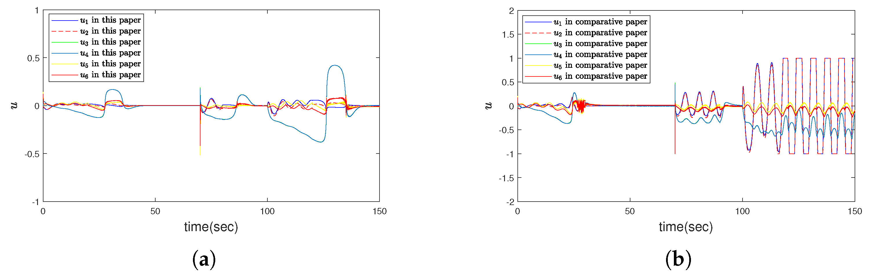
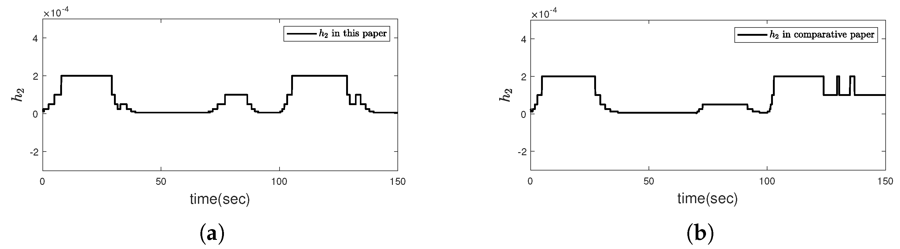
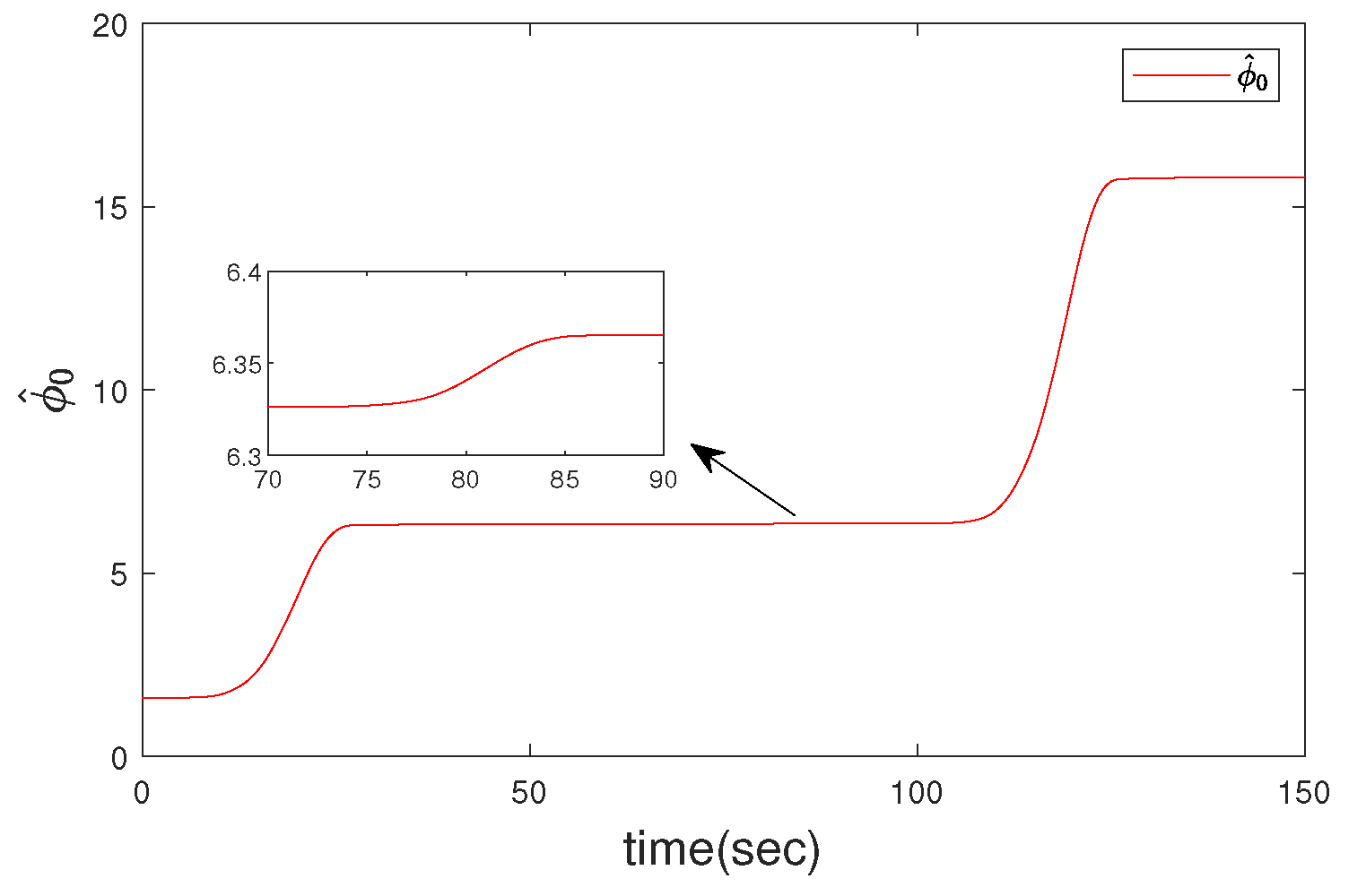
4. Simulation

In this section, simulation experiments are carried out on the classical UMV model, and matlab software is used to verify the superiority of the proposed sliding mode controller. The system matrices for a classical production ship with length L = 200.6 m and mass m = 73,097.15 kg based on [39,40,41] are scaled down to

$$\begin{array}{cc}\hfill & M=\left[\begin{array}{ccc}1.0852& 0& 0\\ 0& 2.0575& -0.4087\\ 0& -0.4087& 0.2153\end{array}\right]\hfill \\ & N=\left[\begin{array}{ccc}0.0865& 0& 0\\ 0& 0.0762& 0.0151\\ 0& 0.0151& 0.031\end{array}\right]\hfill \\ & E=\left[\begin{array}{ccc}0.0389& 0& 0\\ 0& 0.0266& 0\\ 0& 0& 0\end{array}\right]\hfill \\ & \Gamma =\left[\begin{array}{cccccc}1& 1& 0& 0& 0& 0\\ 0& 0& 1& 1& 1& 1\\ 0.0472& -0.0472& -0.4108& -0.3858& 0.4554& 0.3373\end{array}\right]\hfill \end{array}$$

4.1. Simulation Results

The initial state is selected as $e_0=[0.01,-0.01,0.02,0.1,-0.1,0.05]$ and other initial values are chosen: ${h_2}_0=2\times {10}^{-5}$, ${\widehat{\sigma }}_0=[-0.1,-0.3,-0.2,0.3,0.1,0]$, ${\widehat{\overline{u}}}_{s0}=[0,0.1,0.05,-0.05,0.05,-0.01]$, ${\widehat{\psi }}_0=1.6$ and $r_{1i}=r_{2i}=r_{3i}=0.1$. The reference position signals and velocity signals are set to $x_{pd}=y_{pd}={\psi }_d=u_d={\nu }_d=0$, $r_d=\left\{\begin{array}{c}-0.1,0s<t<70s\hfill \\ 0.1,70s<t<150s\hfill \end{array}\right..$ Due to thruster saturation, the controller output amplitude is set to 1, so $u\in [-1,1]$. For the dynamic quantizer, the calculated results of the parameters are $\mho =1.1\times {10}^5$ and $\Im =0.5$, then choose ${\Delta }_1={\Delta }_2=1.1$. The parameters needed to calculate the domain of attraction are $k=13$ solved by a linear matrix expression, $ϵ=0.1$, ${\lambda }_1=12$, fault information parameter $\mu =0.8/0.5/0.2$ under different circumstances.

In order to simulate the UMV in practical application, The fault mode referring to [15,42] is set as follows: when $t\le 70$ s, all six thrusters are working properly; when $t>70$ s, the port main propeller and starboard main propeller are partial fault: the port main propeller has 50 percent of the thrust of normal operation and the starboard main propeller has 30 percent of the thrust of normal operation; Total fault occurs at aft tunnel thruster 1; The rest of thrusters are healthy. The ocean disturbances $w\left(t\right)={[w_1\left(t\right),w_2\left(t\right),w_3\left(t\right)]}^T$ are energy bounded and approaches zero at infinity in [5,43], so let the ocean disturbances occur at two time periods in the simulation: 0–20 s and 100–120 s. It set as $w_1\left(t\right)=0.1*sin\left(t\right)$, $w_2\left(t\right)=0.1$, $w_3\left(t\right)=-0.1*sin\left(t\right)$ in 0–20 s and $w_1\left(t\right)=0.2*sin\left(t\right)$, $w_2\left(t\right)=0.2$, $w_3\left(t\right)=-0.2*sin\left(t\right)$ in 100–120 s.

4.2. Discussion

Compared with the existing paper [15] without considering thruster saturation, the simulation results are shown in Figure 3, Figure 4, Figure 5, Figure 6, Figure 7, Figure 8, Figure 9 and Figure 10. It can be seen from Figure 3a and Figure 4a that under the condition of thruster saturation, fault and ocean disturbance, the error controlled in this paper can asymptotically converge to zero in

Table 1. Amplitude comparison of errors and control laws. ($e_{v1}$ and $e_{\eta 1}$ are amplitude of velocity errors position errors at the final moment; $e_{v2}$ and $e_{\eta 2}$ are amplitude of velocity errors position errors in the process of fluctuation; $\overline{u}$ is amplitude of u in the adjustment process.).

Methods	${\overline{\mathit{e}}}_{\mathit{v}1}$	${\overline{\mathit{e}}}_{\mathsf{\eta }1}$	${\overline{\mathit{e}}}_{\mathit{v}2}$	${\overline{\mathit{e}}}_{\mathsf{\eta }1}$	$\overline{\mathit{u}}$
Method in this paper	$4.5\times {10}^{-4}$	1.7	$2.5\times {10}^{-2}$	11.8	0.41
Method in [15]	1.3	2	1.7	12.3	1

. The disturbance has great influence on the robustness of UMV system. In the simulation, there are two periods of disturbance (0–20 s and 100–120 s). Compared with the first period, the disturbance of the second period is doubled, and it can be seen from the curves and

Table 2. Amplitude comparison of errors under different disturbance periods in this paper. (${\overline{e}}_{v3}$ and ${\overline{e}}_{\eta 3}$ are amplitude of velocity errors position errors in the process of fluctuation; $t_v$ and $t_{\eta }$ are convergence times for velocity and position errors.).

Periods with Disturbance	${\overline{\mathit{e}}}_{\mathit{v}3}$	${\overline{\mathit{e}}}_{\mathsf{\eta }3}$	${\mathit{t}}_{\mathit{v}}$	${\mathit{t}}_{\mathsf{\eta }}$
0–20 s	1.25	8.8	39	40
100–120 s	1.7	11.8	47	42

that the state fluctuation and convergence time of the second stage are significantly larger; But the error oscillations at the last moment of the simulation in Figure 3b and Figure 4b that is caused by the absence of thruster saturation in the controller design in [15], which cannot ensure the stability of the system and cannot maintain the desired position and speed. In particular, the yaw velocity cannot reach the expected velocity, which is reflected in Figure 5b. As shown in Figure 6, when the thruster failure started from 70 s, the sliding mode surface curves under the proposed method in this paper was similar to the error curves, the state could finally reach the $s=0$ and continue to slide on the sliding mode surface; If the controller in [15] is used, the state will fluctuate up and down on both sides of the sliding mode surface. Figure 7 intuitively reflects the comparison of control laws. The results show that the output of the controller in [15] exceeds the output amplitude of the thruster, so the final error convergence cannot be achieved. The changes of dynamic quantization parameter $h_2$ are plotted in Figure 8 respectively, the result shows in Figure 8a that the quantization parameter $h_2$ will adjust to zero contrasts with [15] in Figure 8b. In other words, due to reasonable quantization parameter adjustment, the state can still reach the sliding mode plane in spite of the quantization phenomenon. Figure 9 shows the comparison of parameter $\sigma ,{\overline{u}}_s$: In Figure 9b,d, the control laws u has been growing in fluctuations because the parameters have been increasing without a stable trend and the error e has not approached zero. The ${\widehat{\psi }}_0$ in Figure 10 is exclusive saturation parameter estimation in this paper, which will play an effective role in the controller. Figure 11 presents the domain of attraction with different fault parameter, the fault parameter represents the fault severity of the UMV system. The smaller the parameter is, the bigger the fault is and the smaller the domain of attraction is. It can be seen in Figure 3, Figure 4, Figure 5, Figure 6, Figure 7, Figure 8, Figure 9, Figure 10 and Figure 11 that using the proposed method not only makes the UMV system stable, but also reveals the extent of the domain of attraction. Therefore, the superiority of the controller designed in this paper is clearly proved through the above comparison curves.

5. Conclusions

A new sliding mode control method is proposed to solve the thruster failure and saturation problems for UMVs system with state quantization and input signal quantization. When thruster redundancy exists in UMVs system, sliding mode control strategy is integrated with adaptive mechanism, and the designed controller can compensate the quantization error, thruster saturation and thruster failure. This method does not require the fault detection and isolation mechanism to directly compensate some faults of steering gear. Furthermore, a more lager adjustment range of quantization parameter is revealed to ensure the accessibility. Under the influence of quantization, the control law makes the state reach the region near the sliding surface (the banded region), and then the state is asymptotically zero by the adjustment of the quantization parameters. Finally, the effectiveness of the proposed sliding mode controller is verified by simulation. The limitations of this paper are the dynamic quantification of thruster input and the time-varying delay of state output for UMV system. In the future, input quantizer parameter adjustment strategy and construction of a new UMV model with time-varying delay will be discussed.

References

- Fossen, T.I. Guidance and control of ocean vehicles. Automatica 1996, 32, 1235. [Google Scholar]
- Guze, S.; Wawrzynski, W.; Wilczynski, P. Determination of parameters describing the risk areas of ships chaotic rolling on the example of LNG carrier and OSV vessel. J. Mar. Sci. Eng. 2020, 8, 91. [Google Scholar] [CrossRef]
- Li, Y.X.; Yang, G.H. Adaptive asymptotic tracking control of uncertain nonlinear systems with input quantization and actuator faults. Automatica 2016, 72, 177–185. [Google Scholar] [CrossRef]
- Guo, X.G.; Wang, J.L.; Liao, F. Adaptive quantised observer-based output feedback control for non-linear systems with input and output quantisation. IET Control. Theory Appl. 2017, 11, 263–272. [Google Scholar] [CrossRef]
- Hao, L.Y.; Yu, Y.; Li, T.S.; Li, H. Quantized output-feedback control for unmanned marine vehicles with thruster faults via sliding-mode technique. IEEE Trans. Cybern. 2022, 52, 9363–9376. [Google Scholar] [CrossRef]
- Ye, Z.; Zhang, D.; Cheng, J.; Wu, Z.G. Event-triggering and quantized sliding mode control of UMV systems under dos attack. IEEE Trans. Veh. Technol. 2022, 71, 8199–8211. [Google Scholar] [CrossRef]
- Zhou, B.; Su, Y.M.; Huang, B.; Wang, W.; Zhang, E. Trajectory tracking control for autonomous underwater vehicles under quantized state feedback and ocean disturbances. Ocean. Eng. 2022, 256, 111500. [Google Scholar] [CrossRef]
- Yan, Y.; Yu, S.H. Sliding mode tracking control of autonomous underwater vehicles with the effect of quantization. Ocean. Eng. 2018, 151, 322–328. [Google Scholar] [CrossRef]
- An, S.; Wang, L.; He, Y. Adaptive backstepping sliding mode tracking control for autonomous underwater vehicles with input quantization. Adv. Theory Simulations 2022, 5, 2100445. [Google Scholar] [CrossRef]
- Yan, Y.; Yu, S.; Yu, S. Quantized super-twisting algorithm based sliding mode control. Automatica 2019, 105, 43–48. [Google Scholar] [CrossRef]
- Cheng, Y.; Liu, T.; Weng, R. Sliding mode control of continuous-time switched systems with signal quantization and actuator nonlinearit. Sci. Prog. 2020, 103, 1–21. [Google Scholar] [CrossRef] [PubMed]
- Liu, M.; Zhang, L.X.; Shi, P.; Zhao, Y. Sliding mode control of continuous-time markovian jump systems with digital data transmission. Automatica 2017, 80, 200–209. [Google Scholar] [CrossRef]
- Wang, Y.; Jiang, B.; Wu, Z.G.; Xie, S.; Peng, Y. Adaptive sliding mode fault-tolerant fuzzy tracking control with application to unmanned marine vehicles. IEEE Trans. Syst. Man Cybern. Syst. 2021, 51, 6691–6700. [Google Scholar] [CrossRef]
- Ma, H.; Zhou, Q.; Bai, L.; Liang, H. Observer-based adaptive fuzzy fault-tolerant control for stochastic nonstrict-feedback nonlinear systems with input quantization. IEEE Trans. Syst. Man Cybern. Syst. 2019, 49, 287–298. [Google Scholar] [CrossRef]
- Hao, L.Y.; Zhang, H.; Li, H.; Li, T.S. Sliding mode fault-tolerant control for unmanned marine vehicles with signal quantization and time-delay. Ocean. Eng. 2020, 215, 107882. [Google Scholar] [CrossRef]
- Cavanini, L.; Ippoliti, G. Fault tolerant model predictive control for an over-actuated vessel. Ocean. Eng. 2018, 160, 1–9. [Google Scholar] [CrossRef]
- Najafi, A.; Vu, M.T.; Mobayen, S.; Asad, J.H.; Fekih, A. Adaptive barrier fast terminal sliding mode actuator fault tolerant control approach for quadrotor UAVs. Mathematics 2022, 10, 3009. [Google Scholar] [CrossRef]
- Ao, W.; Song, Y.D.; Wen, C.Y. Adaptive robust fault tolerant control design for a class of nonlinear uncertain MIMO systems with quantization. ISA Trans. 2017, 68, 63–72. [Google Scholar] [CrossRef]
- Chen, L.; Fu, S.; Zhao, Y. Fault-tolerant control for unmanned surface vehicles with digital communication channel. In Advances in Guidance, Navigation and Control; Springer: Singapore, 2022; pp. 1589–1597. [Google Scholar]
- Li, M.; Shi, P.; Liu, M. Event-triggered-based adaptive sliding mode control for T–S fuzzy systems with actuator failures and signal quantization. IEEE Trans. Fuzzy Syst. 2021, 29, 1363–1374. [Google Scholar] [CrossRef]
- Shi, P.; Liu, M.; Zhang, L. Fault-tolerant sliding-mode-observer synthesis of markovian jump systems using quantized measurements. IEEE Trans. Ind. Electron. 2015, 62, 5910–5918. [Google Scholar] [CrossRef]
- Chen, L.; Liu, M.; Huang, X.; Fu, S.; Qiu, J. Adaptive fuzzy sliding mode control for network-based nonlinear systems with actuator failures. IEEE Trans. Fuzzy Syst. 2018, 26, 1311–1323. [Google Scholar] [CrossRef]
- Vu, M.T.; Le, T.H.; Thanh, H.N. Robust position control of an over-actuated underwater vehicle under model uncertainties and ocean current effects using dynamic sliding mode surface and optimal allocation control. Sensors 2021, 21, 747. [Google Scholar] [CrossRef]
- Wang, N.; Deng, Z. Finite-time fault estimator based fault-tolerance control for a surface vehicle with input saturations. IEEE Trans. Ind. Inform. 2020, 16, 1172–1181. [Google Scholar] [CrossRef]
- Su, Y.; Zheng, C.; Mercorelli, P. Nonlinear pd fault tolerant control for dynamic positioning of ships with actuator constraints. IEEE/ASME Trans. Mech. 2017, 22, 1132–1142. [Google Scholar] [CrossRef]
- Ghaffari, V.; Mobayen, S.; ud Din, S.; Rojsiraphisal, T.; Vu, M.T. Robust tracking composite nonlinear feedback controller design for time-delay uncertain systems in the presence of input saturatio. ISA Trans. 2022, 129, 88–99. [Google Scholar] [CrossRef]
- Hu, J.; Ghaffari, V.; Mobayen, S.; Asad, J.H.; Vu, M.T. Robust composite nonlinear feedback control based on integral sliding-mode control of uncertain time-delay systems under input saturation. J. Vib. Control. 2022. [Google Scholar] [CrossRef]
- Hao, L.Y.; Yang, G.H. Fault-tolerant control via sliding-mode output feedback for uncertain linear systems with quantisation. IET Control. Theory Appl. 2013, 7, 1992–2006. [Google Scholar] [CrossRef]
- Zheng, B.C.; Yang, G.H. Quantised feedback stabilisation of planar systems via switching-based sliding-mode control. IET Control. Theory Appl. 2012, 6, 149–156. [Google Scholar] [CrossRef]
- Fossen, T.I. Marine Control Systems: Guidance, Navigation and Control of Ships, Rigs and Underwater Vehicles; Marine Cybernetics: Trondheim, Norway, 2002; ISBN 8292356002. [Google Scholar]
- Zhu, Z.; Xia, Y.Q.; Fu, M.Y. Adaptive sliding mode control for attitude stabilization with actuator saturation. IEEE Trans. Ind. Electron. 2011, 58, 4898–4907. [Google Scholar] [CrossRef]
- Xue, Y.; Zheng, B.C.; Yu, X. Robust sliding mode control for TS fuzzy systems via quantized state feedback. IEEE Trans. Fuzzy Syst. 2017, 26, 2261–2272. [Google Scholar] [CrossRef]
- Hao, L.Y.; Zhang, H.; Li, T.S.; Lin, B.; Chen, C.L.P. Fault Tolerant Control for Dynamic Positioning of Unmanned Marine Vehicles based on T-S Fuzzy Model with Unknown Membership Functions. IEEE Trans. Veh. Technol. 2021, 70, 146–157. [Google Scholar] [CrossRef]
- Hao, L.Y.; Zhang, H.; Guo, G.; Li, H. Quantized Sliding Mode Control of Unmanned Marine Vehicles: Various Thruster Faults Tolerated With a Unified Model. IEEE Trans. Syst. Man Cybern. Syst. 2021, 51, 2012–2026. [Google Scholar] [CrossRef]
- Alattas, K.A.; Vu, M.T.; Mofid, O.; El-Sousy, F.F.; Alanazi, A.K.; Awrejcewicz, J.; Mobayen, S. Adaptive nonsingular terminal sliding mode control for performance improvement of perturbed nonlinear systems. Mathematics 2022, 10, 1064. [Google Scholar] [CrossRef]
- Han, H.C. An analysis and design method for uncertain variable. IEEE Trans. Autom. Control. 2004, 49, 602–607. [Google Scholar]
- Hao, L.Y.; Yang, G.H. Fault tolerant control for a class of uncertain chaotic systems with actuator saturation. Nonlinear Dyn. 2013, 73, 2133–2147. [Google Scholar] [CrossRef]
- Matallana, L.G.; Blanco, A.M.; Bandoni, J.A. Nonlinear dynamic systems design based on the optimization of the domain of attraction. Math. Comput. Model. 2011, 53, 731–745. [Google Scholar] [CrossRef]
- Kahveci, N.E.; Ioannou, P.A. Adaptive steering control for uncertain ship dynamics and stability analysis. Automatica 2013, 49, 685–697. [Google Scholar] [CrossRef]
- Wang, Y.L.; Han, Q.L. Network-based modelling and dynamic output feedback control for unmanned marine vehicles in network environments. Automatica 2018, 91, 43–53. [Google Scholar] [CrossRef]
- Fossen, T.I.; Sagatun, S.I.; Sørensen, A.J. Identification of dynamically positioned ships. Control. Eng. Pract. 1996, 4, 369–376. [Google Scholar] [CrossRef]
- Huang, H.; Wan, L.; Chang, W.; Pang, Y.; Jiang, S. A fault-tolerable control scheme for an open-frame underwater vehicle. Int. J. Adv. Robot. Syst. 2014, 11, 77. [Google Scholar] [CrossRef]
- Yang, G.H.; Ye, D. Reliable H∞ control of linear systems with adaptive mechanism. IEEE Trans. Autom. Control. 2010, 55, 242–247. [Google Scholar] [CrossRef]