
Study on Meso-Structural Evolution of Bedrock Beneath Offshore Wind Turbine Foundation in Pressurized Seawater


Abstract
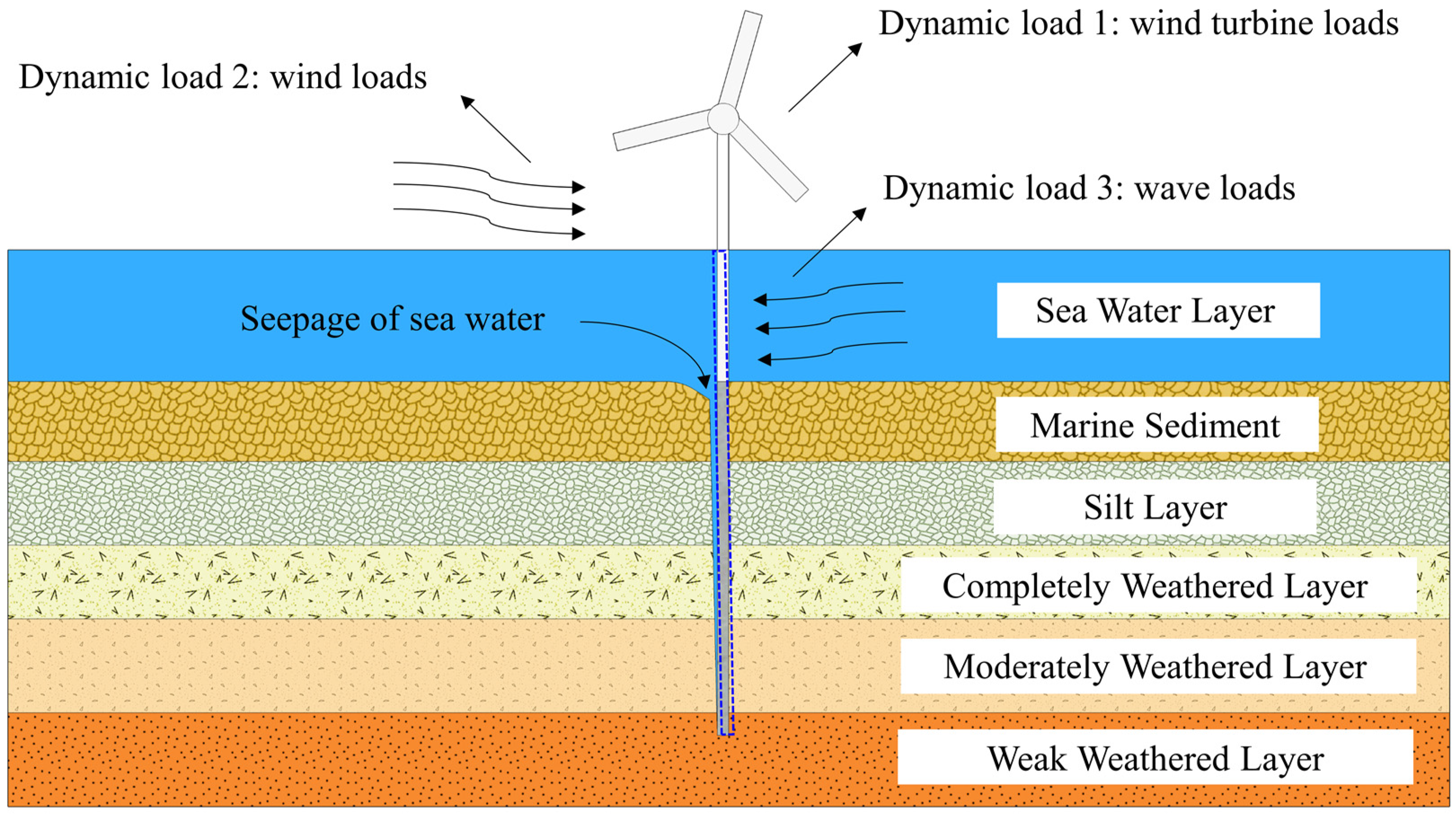
:1. Introduction
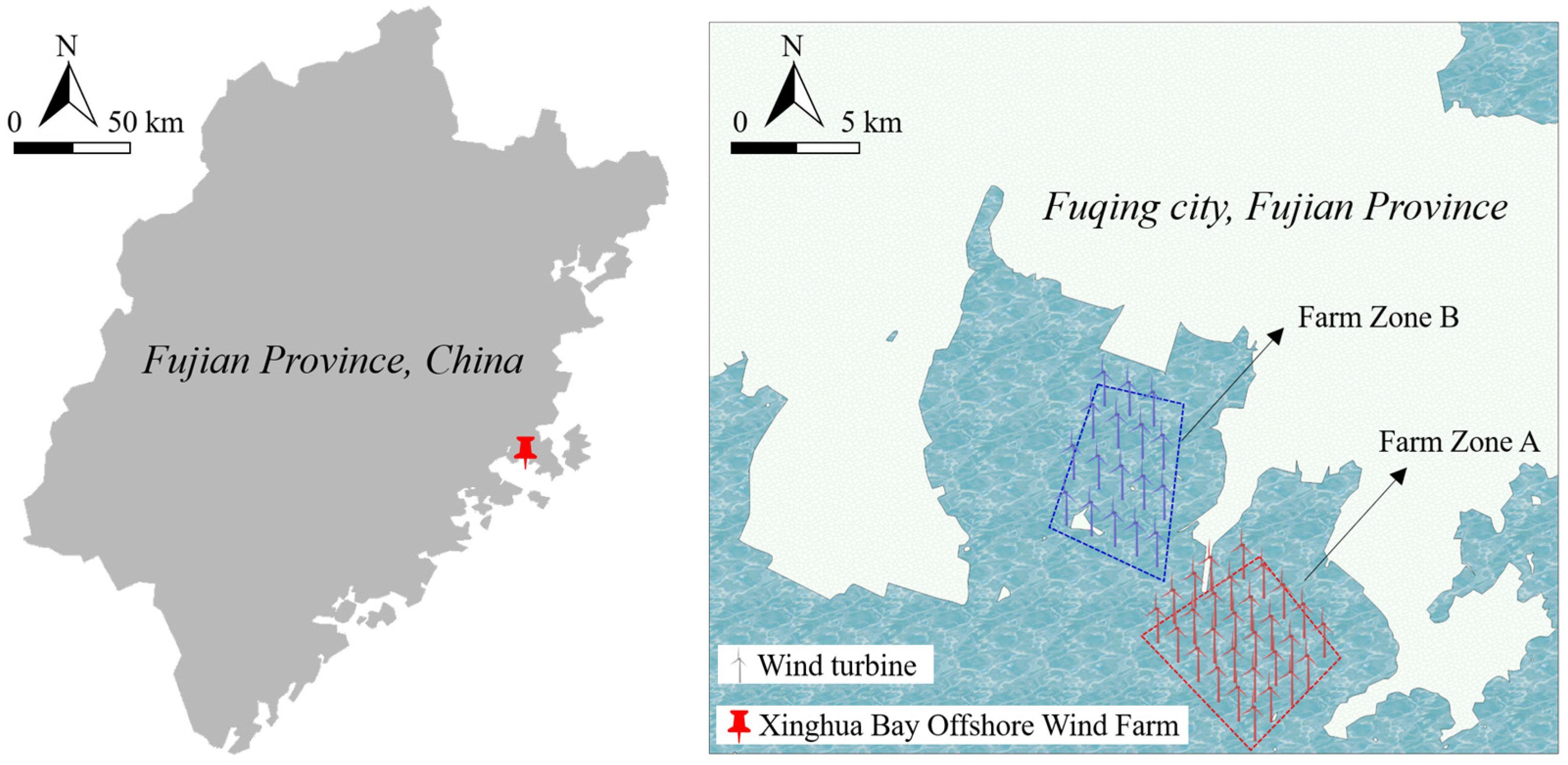
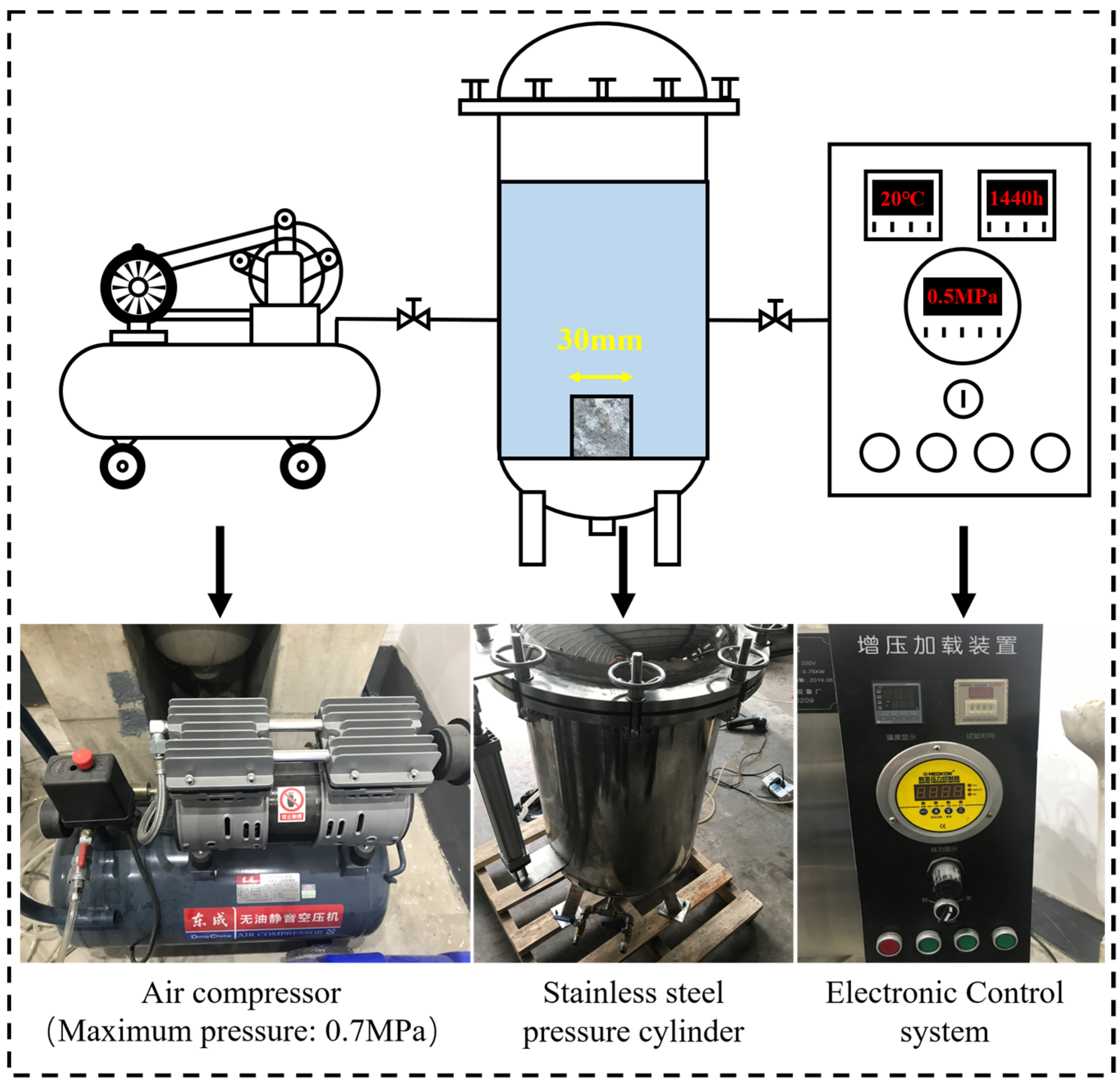
2. Methodology and Materials
2.1. Preparation of Rock Samples
2.2. CT Scanning Test
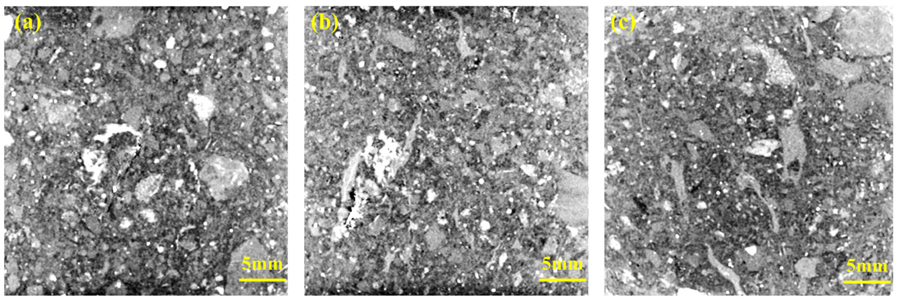
3. Analysis of Meso-Structural Evolution of Tuff
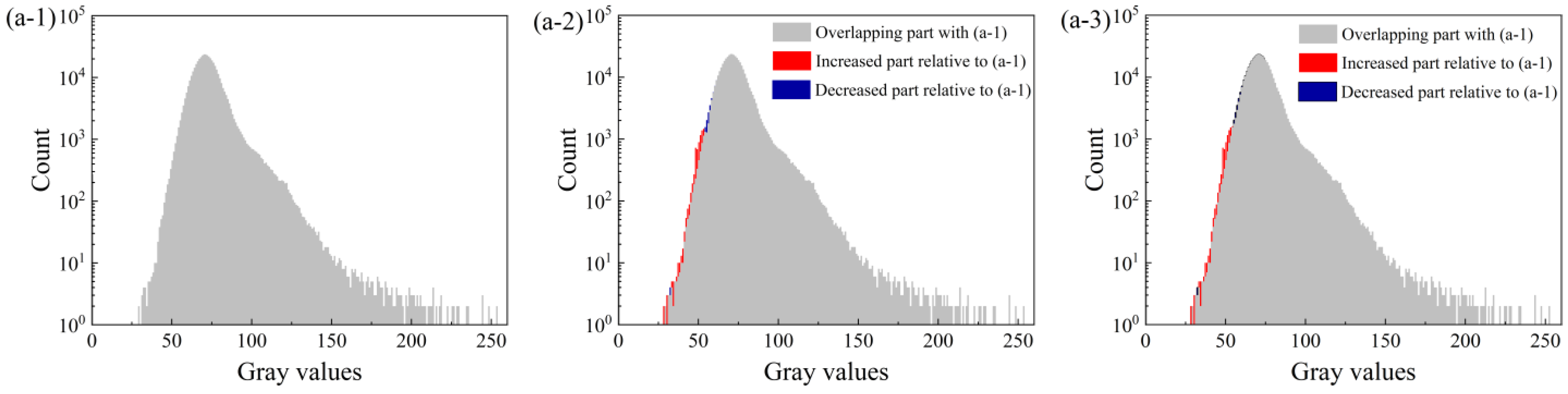
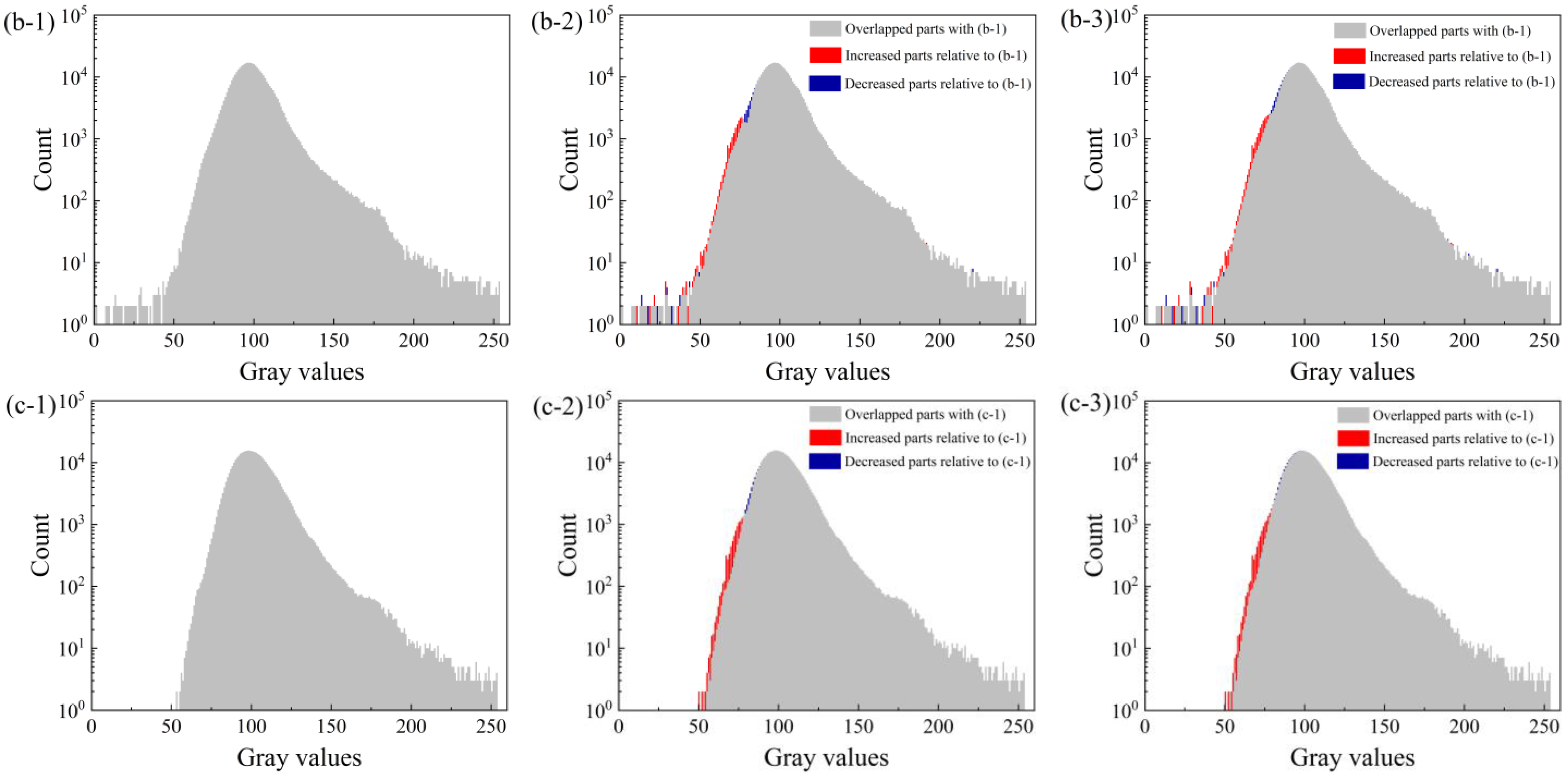
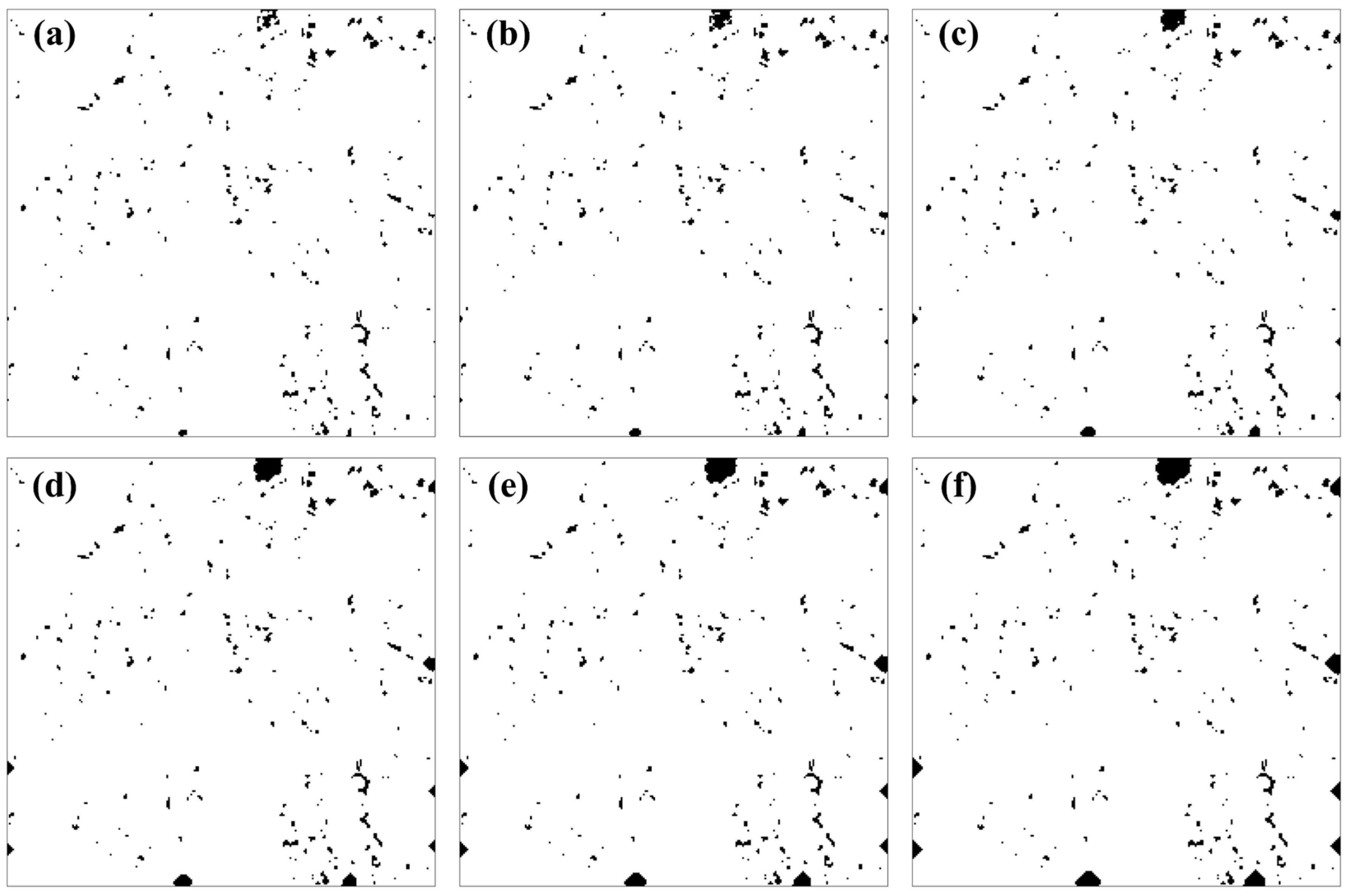
3.1. Two-Dimensional Analysis Based on CT Slices
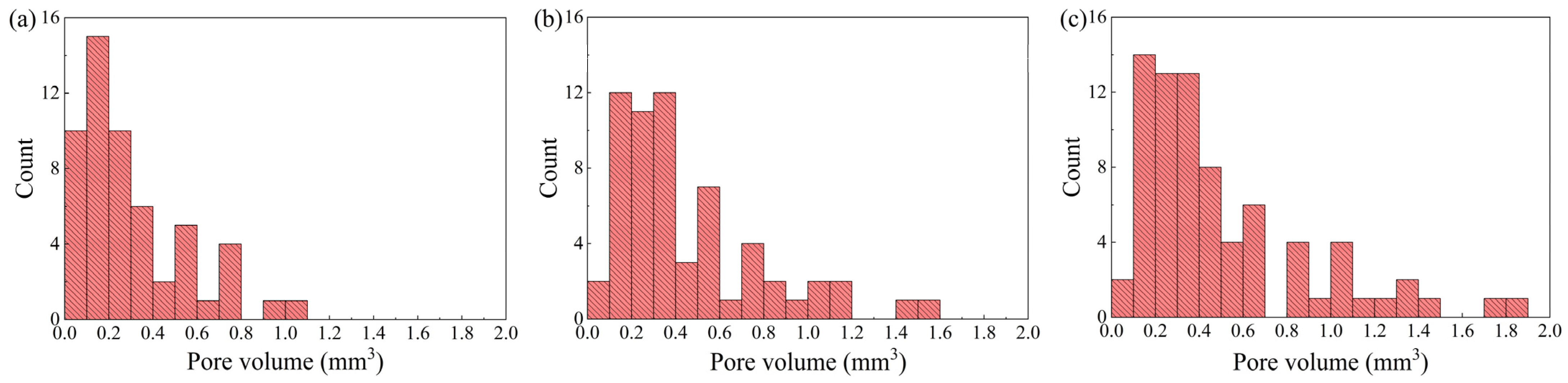
3.2. Three-Dimensional analysis Based on Pore Model
4. Prediction of Long-Term Deterioration by Cellular Automata
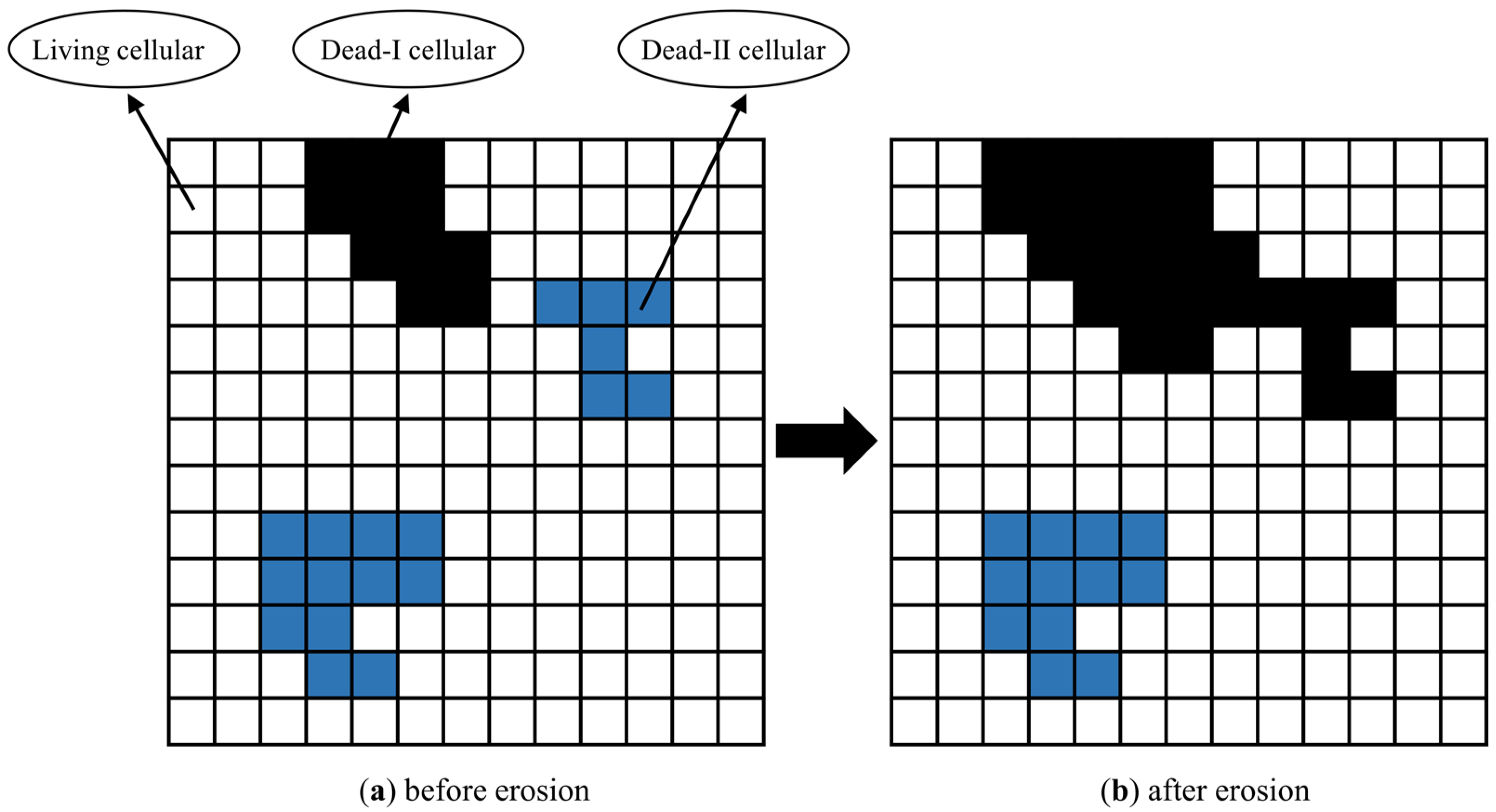
4.1. Model Concept and Governing Equations in Cellular Automata
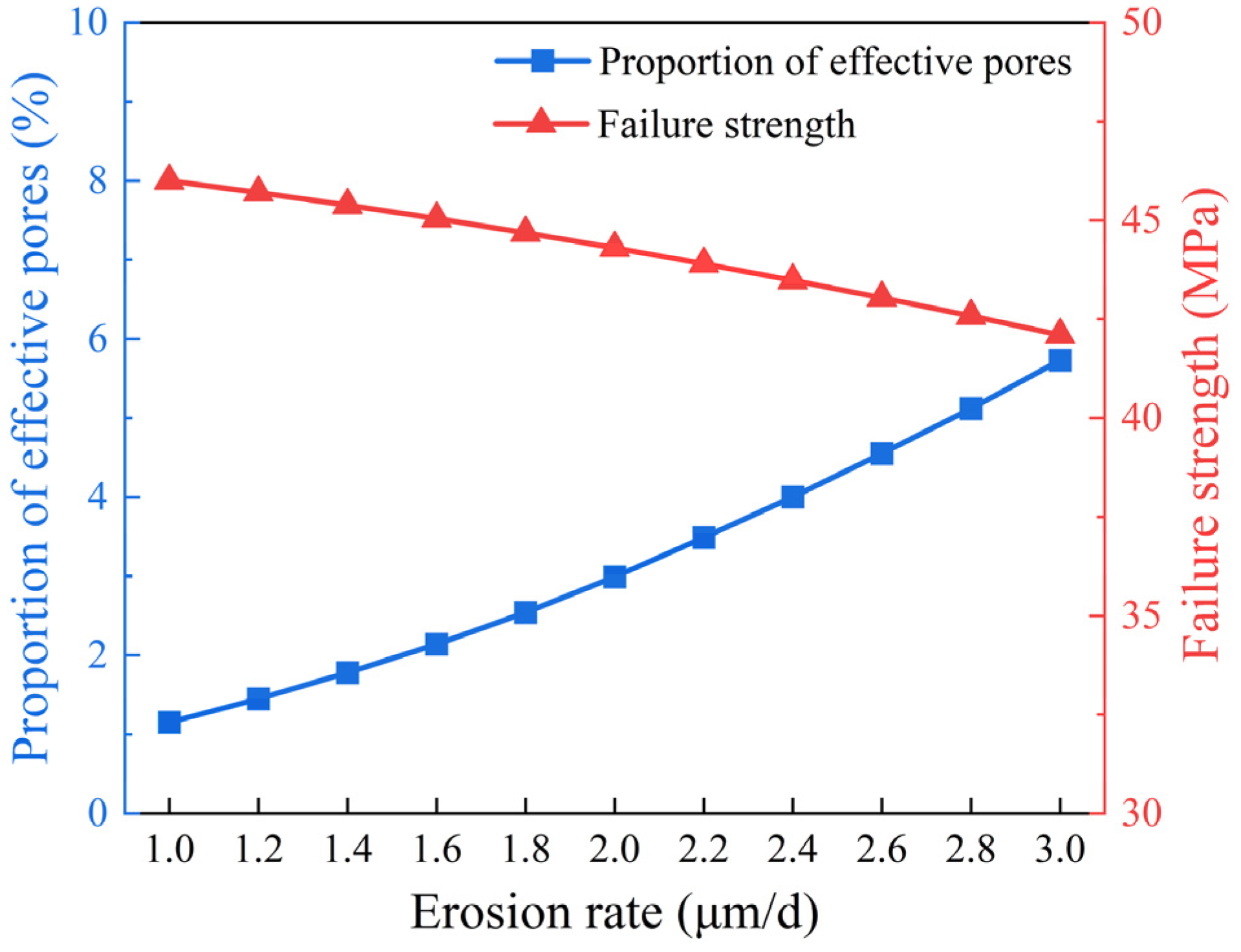
4.2. Numerical Results and Discussion
5. Conclusions
Author Contributions
Funding
Institutional Review Board Statement
Informed Consent Statement
Data Availability Statement
Acknowledgments
Conflicts of Interest
References
- Kallehave, D.; Byrne, B.W.; Leblanc Thilsted, C.; Mikkelsen, K.K. Optimization of monopiles for offshore wind turbines. Philos. Trans. R. Soc. A Math. Phys. Eng. Sci. 2015, 373, 20140100. [Google Scholar] [CrossRef] [PubMed]
- Esteban, M.D.; Couñago, B.; López-Gutiérrez, J.S.; Negro, V.; Vellisco, F. Gravity based support structures for offshore wind turbine generators: Review of the installation process. Ocean Eng. 2015, 110, 281–291. [Google Scholar] [CrossRef]
- Shi, W.; Park, H.; Chung, C.; Baek, J.; Kim, Y.; Kim, C. Load analysis and comparison of different jacket foundations. Renew. Energy 2013, 54, 201–210. [Google Scholar] [CrossRef]
- Zhang, Q.; Zhang, C.; Lin, Y.; Li, Y.; Shen, Y.; Pei, Y. Experimental study on deterioration of bedrock strength and p-wave velocity by pressurized seawater. Geomech. Geophys. Geo-Energy Geo-Resour. 2023, 9, 121. [Google Scholar] [CrossRef]
- Zhang, Y.; Liao, C.; Chen, J.; Tong, D.; Wang, J. Numerical analysis of interaction between seabed and mono-pile subjected to dynamic wave loadings considering the pile rocking effect. Ocean Eng. 2018, 155, 173–188. [Google Scholar] [CrossRef]
- Zhu, B.; Ren, J.; Ye, G. Wave-induced liquefaction of the seabed around a single pile considering pile-soil interaction. Mar. Georesour. Geotechnol. 2018, 36, 150–162. [Google Scholar] [CrossRef]
- Liu, Z.; He, X.; Fan, J.; Zhou, C. Study on the softening mechanism and control of red-bed soft rock under seawater conditions. J. Mar. Sci. Eng. 2019, 7, 235. [Google Scholar] [CrossRef]
- Ma, D.; Duan, H.Y.; Li, X.B.; Li, Z.H.; Zhou, Z.L.; Li, T.B. Effects of seepage-induced erosion on nonlinear hydraulic properties of broken red sandstones. Tunn. Undergr. Space Technol. 2019, 91, 102993. [Google Scholar] [CrossRef]
- Wu, C.; Hong, Y.; Chen, Q.; Karekal, S. A modified optimization algorithm for back analysis of properties for coupled stress-seepage field problems. Tunn. Undergr. Space Technol. 2019, 94, 103040. [Google Scholar] [CrossRef]
- Zhou, Z.L.; Cai, X.; Cao, W.Z.; Li, X.B.; Xiong, C. Influence of water content on mechanical properties of rock in both saturation and drying processes. Rock Mech. Rock Eng. 2016, 49, 3009–3025. [Google Scholar] [CrossRef]
- Goudie, A.S. Experimental salt weathering of limestones in relation to rock properties. Earth Surf. Proc. Land. 1999, 24, 715–724. [Google Scholar] [CrossRef]
- Heggheim, T.; Madland, M.V.; Risnes, R.; Austad, T. A chemical induced enhanced weakening of chalk by seawater. J. Petrol. Sci. Eng. 2005, 46, 171–184. [Google Scholar] [CrossRef]
- Risnes, R.; Haghighi, H.; Korsnes, R.I.; Natvik, O. Chalk-fluid interactions with glycol and brines. Tectonophysics 2003, 370, 213–226. [Google Scholar] [CrossRef]
- Wang, J.; Feng, B.; Zhang, X.; Tang, Y.; Yang, P. Hydraulic failure mechanism of karst tunnel surrounding rock. Chin. J. Rock Mech. Eng. 2010, 29, 1363–1370. [Google Scholar]
- Liu, Y.; Liu, C.W.; Kang, Y.M.; Wang, D.; Ye, D.Y. Experimental research on creep properties of limestone under fluid-solid coupling. Environ. Earth Sci. 2015, 73, 7011–7018. [Google Scholar] [CrossRef]
- Zhang, G.L.; Ranjith, P.C.; Perera, M.S.A.; Lu, Y.; Choi, X. Quantitative analysis of micro-structural changes in a bituminous coal after exposure to supercritical CO2 and water. Nat. Resour. Res. 2019, 28, 1639–1660. [Google Scholar] [CrossRef]
- Bandara, K.M.A.S.; Ranjith, P.G.; Haque, A.; Wanniarachchi, W.A.M.; Zheng, W.; Rathnaweera, T.D. An experimental investigation of the effect of long-term, time-dependent proppant embedment on fracture permeability and fracture aperture reduction. Int. J. Rock Mech. Min. 2021, 144, 104813. [Google Scholar] [CrossRef]
- Chen, B.; Xiang, J.; Latham, J.; Bakker, R.R. Grain-scale failure mechanism of porous sandstone: An experimental and numerical FDEM study of the Brazilian tensile strength test using CT-scan microstructure. Int. J. Rock Mech. Min. 2020, 132, 104348. [Google Scholar] [CrossRef]
- Zhuang, L.; Kim, K.Y.; Jung, S.G.; Diaz, M.; Min, K.; Zang, A.; Stephansson, O.; Zimmerman, G.; Yoon, J.; Hofmann, H. Cyclic hydraulic fracturing of pocheon granite cores and its impact on breakdown pressure, acoustic emission amplitudes and injectivity. Int. J. Rock Mech. Min. 2019, 122, 104065. [Google Scholar] [CrossRef]
- Li, T.; Yang, B.; Qi, Z.; Gu, C.; Shan, Q.; Chen, W. Numerical simulation of roof movement and fill strength of coal deep mining. Arab. J. Geosci. 2021, 14, 665. [Google Scholar] [CrossRef]
- Xu, W.; Yue, Z.; Hu, R. Study on the mesostructure and mesomechanical characteristics of the soil-rock mixture using digital image processing based finite element method. Int. J. Rock Mech. Min. 2008, 45, 749–762. [Google Scholar] [CrossRef]
- Helmons, R.L.J.; Miedema, S.A.; van Rhee, C. Simulating hydro mechanical effects in rock deformation by combination of the discrete element method and the smoothed particle method. Int. J. Rock Mech. Min. 2016, 86, 224–234. [Google Scholar] [CrossRef]
- Jiang, M.; Chen, H.; Crosta, G.B. Numerical modeling of rock mechanical behavior and fracture propagation by a new bond contact model. Int. J. Rock Mech. Min. 2015, 78, 175–189. [Google Scholar] [CrossRef]
- Regassa, B.; Xu, N.; Mei, G. An equivalent discontinuous modeling method of jointed rock masses for dem simulation of mining-induced rock movements. Int. J. Rock Mech. Min. 2018, 108, 1–14. [Google Scholar] [CrossRef]
- Xu, W.; Hu, L.; Gao, W. Random generation of the meso-structure of a soil-rock mixture and its application in the study of the mechanical behavior in a landslide dam. Int. J. Rock Mech. Min. 2016, 86, 166–178. [Google Scholar] [CrossRef]
- Biswas, K.; Vasant, P.M.; Vintaned, J.A.G.; Watada, J. Cellular automata-based multi-objective hybrid grey wolf optimization and particle swarm optimization algorithm for wellbore trajectory optimization. J. Nat. Gas Sci. Eng. 2021, 85, 103695. [Google Scholar] [CrossRef]
- Mei, W.; Li, M.; Pan, P.; Pan, J.; Liu, K. Blasting induced dynamic response analysis in a rock tunnel based on combined inversion of Laplace transform with elasto-plastic cellular automaton. Geophys. J. Int. 2021, 225, 699–710. [Google Scholar] [CrossRef]
- Castro, R.; Gomez, R.; Arancibia, L. Fine material migration modelled by cellular automata. Granul. Matter. 2022, 24, 14. [Google Scholar] [CrossRef]
- Feng, X.; Pan, P.; Zhou, H. Simulation of the rock microfracturing process under uniaxial compression using an elasto-plastic cellular automaton. Int. J. Rock Mech. Min. 2006, 43, 1091–1108. [Google Scholar] [CrossRef]
- Pan, P.; Feng, X.; Hudson, J.A. Numerical simulations of class i and class ii uniaxial compression curves using an elasto-plastic cellular automaton and a linear combination of stress and strain as the control method. Int. J. Rock Mech. Min. 2006, 43, 1109–1117. [Google Scholar] [CrossRef]
- Pan, P.; Feng, X.; Hudson, J.A. Study of failure and scale effects in rocks under uniaxial compression using 3d cellular automata. Int. J. Rock Mech. Min. 2009, 46, 674–685. [Google Scholar] [CrossRef]
- Huang, X.; Hayashi, K.; Fujii, M. Resources time footprint analysis of onshore wind turbines combined with GIS-based site selection: A case study in Fujian province, China. Energy Sustain. Dev. 2023, 74, 102–114. [Google Scholar] [CrossRef]
- Gong, W.; Zhang, Z.; Lin, Y.; Dai, G.; Huang, H. Full-scale field test study of bearing characteristics of post-grouting pile for offshore wind turbines. Ocean Eng. 2023, 268, 113451. [Google Scholar] [CrossRef]
- Xu, Z.T.; Yang, Q.F.; Sun, J.G.; Lei, F.Z.; Pan, X.D.; Li, Z.W. Origin of late jurassic high-kfelsic volcanic rocks and related au mineralization in the Dongyang deposit, central-eastern Fujian, SEChina, and its tectonic implications. Geol. J. 2021, 56, 572–598. [Google Scholar] [CrossRef]
- Zhang, C.H.; Zhang, Q.; Liu, J.; Tian, L.G.; Dai, G.L. Experimental research on mechanical property of granite under erosion by seawater. IOP Conf. Ser. Earth Environ. Sci. 2020, 570, 32010–32040. [Google Scholar] [CrossRef]
- Andrushia, D.; Anand, N.; Arulraj, P. Anisotropic diffusion based denoising on concrete images and surface crack segmentation. Int. J. Struct. Integr. 2020, 11, 395–409. [Google Scholar] [CrossRef]
- Zhou, Y.Y.; Lin, M.S.; Xu, S.; Zang, H.B.; He, H.S.; Li, Q.; Guo, J. An image denoising algorithm for mixed noise combining nonlocal means filter and sparse representation technique. J. Vis. Commun. Image Represent. 2016, 41, 74–86. [Google Scholar] [CrossRef]
- Eldib, M.E.; Hegazy, M.; Mun, Y.J.; Cho, M.H.; Cho, M.H.; Lee, S.Y. A ring artifact correction method: Validation by micro-CT imaging with flat-panel detectors and a 2d photon-counting detector. Sensors 2017, 17, 269. [Google Scholar] [CrossRef]
- Podgorsak, A.R.; Nagesh, S.V.S.; Bednarek, D.; Rudin, S.; Ionita, C.N. Use of a cmos-based micro-CT system to validate a ring artifact correction algorithm on low-dose image data. In Proceedings of the SPIE Medical Imaging, Houston, TX, USA, 10–15 February 2018; p. 10573. [Google Scholar] [CrossRef]
- Wang, G.; Shen, J.; Liu, S.; Jiang, C.; Qin, X. Three-dimensional modeling and analysis of macro-pore structure of coal using combined x-ray CT imaging and fractal theory. Int. J. Rock Mech. Min. 2019, 123, 104082. [Google Scholar] [CrossRef]
- Blunt, M.J. Flow in porous media—Pore-network models and multiphase flow. Curr. Opin. Colloid Interface Sci. 2001, 6, 197–207. [Google Scholar] [CrossRef]
- Al-Zboon, K.K.; Zou’By, J. Natural volcanic tuff for sustainable concrete industry. Jordan J. Civ. Eng. 2017, 11, 408–423. [Google Scholar]
- Guadagnuolo, M.; Aurilio, M.; Basile, A.; Faella, G. Modulus of elasticity and compressive strength of tuff masonry: Results of a wide set of flat-jack tests. Buildings 2020, 10, 84. [Google Scholar] [CrossRef]
- Kayabasi, A.; Gokceoglu, C. Deformation modulus of rock masses: An assessment of the existing empirical equations. Geotech. Geol. Eng. 2018, 36, 2683–2699. [Google Scholar] [CrossRef]
- Sonmez, H.; Tuncay, E.; Gokceoglu, C. Models to predict the uniaxial compressive strength and the modulus of elasticity for Ankara agglomerate. Int. J. Rock Mech. Min. 2004, 41, 717–729. [Google Scholar] [CrossRef]
- Togashi, Y.; Kikumoto, M.; Tani, K.; Hosoda, K.; Ogawa, K. Detection of deformation anisotropy of tuff by a single triaxial test on a single specimen. Int. J. Rock Mech. Min. 2018, 108, 23–36. [Google Scholar] [CrossRef]
- Wang, J.; Chen, X.; Wei, M.; Dai, F. Triaxial fatigue behavior and acoustic emission characteristics of saturated tuff. Int. J. Geomech. 2021, 21, 04021230. [Google Scholar] [CrossRef]


| Mineral Classification | Content | |
|---|---|---|
| Crystal pyroclast | Plagioclase | 15% |
| Quartz | 10% | |
| Alkali feldspar | 8% | |
| White mica | 4% | |
| Chalcedony | 3% | |
| Cuttings | 35% | |
| Vitroclastic texture | 15% | |
| Interstitial material | 10% | |
| Test Items | Unit | Value | Limit of Detection |
|---|---|---|---|
| K+ | mg/L | 539 | 0.05 |
| Ca2+ | 441 | 0.02 | |
| Na+ | 8.70 × 10³ | 0.03 | |
| Mg2+ | 1.05 × 10³ | 0.003 | |
| Cl− | 1.76 × 10⁴ | 0.007 | |
| SO42− | 4.63 × 10³ | 0.018 | |
| CO32− | 5.2 | 0.3 | |
| HCO32− | 104 | 0.6 |
| Model | Y. CT Precision S | |
|---|---|---|
| Operation modes | CT | Volume scan (Cone beam geometry) |
| DR | Digital radiography | |
| Scan time | CT | Typical 10~30 min |
| DR | Max 7.5 frames/sec | |
| Max. tube power | 320 W | |
| High voltage range | 10~225 kV | |
| Tube current | 0.01~3.0 mA | |
| Pixel number | 10242 Pixel | |
| Environment | Time | Pore Volume/mm3 | Porosity/% | Amplification/% |
|---|---|---|---|---|
| Pure water (OP) | Before immersion | 413.52 | 1.53 | --- |
| 30th day | 419.83 | 1.55 | 1.53 | |
| 60th day | 424.17 | 1.57 | 2.58 | |
| Seawater (OP) | Before immersion | 347.61 | 1.29 | --- |
| 30th day | 353.09 | 1.31 | 1.58 | |
| 60th day | 356.18 | 1.32 | 2.47 | |
| Pressurized seawater (0.5 MPa) | Before immersion | 362.23 | 1.34 | --- |
| 30th day | 381.76 | 1.41 | 5.39 | |
| 60th day | 393.51 | 1.46 | 8.64 |
| Notation | Value | Unit | Description |
|---|---|---|---|
| m | 250 | 1 | Number of cells per row |
| n | 250 | 1 | Number of cells per column |
| a | 0.2 | mm | Length of each cell |
| v | 1 | μm/d | Normal erosion rate |
| e | 45 | GPa | Elastic modulus of undamaged tuff |
| m | 5 | 1 | Homogeneity index of rock |
| 3 | 1 | Average failure thresholds of cells | |
| E(t) | 1 | 1 | Input energy in the model at time t |
| f(T) | f(T) | 1 | Reduction coefficient of the failure thresholds |
Disclaimer/Publisher’s Note: The statements, opinions and data contained in all publications are solely those of the individual author(s) and contributor(s) and not of MDPI and/or the editor(s). MDPI and/or the editor(s) disclaim responsibility for any injury to people or property resulting from any ideas, methods, instructions or products referred to in the content. |
© 2023 by the authors. Licensee MDPI, Basel, Switzerland. This article is an open access article distributed under the terms and conditions of the Creative Commons Attribution (CC BY) license (https://creativecommons.org/licenses/by/4.0/).
Share and Cite
Zhang, Q.; Zhang, C.; Lin, Y.; Li, Y.; Shen, Y.; Pei, Y. Study on Meso-Structural Evolution of Bedrock Beneath Offshore Wind Turbine Foundation in Pressurized Seawater. J. Mar. Sci. Eng. 2023, 11, 2260. https://doi.org/10.3390/jmse11122260
Zhang Q, Zhang C, Lin Y, Li Y, Shen Y, Pei Y. Study on Meso-Structural Evolution of Bedrock Beneath Offshore Wind Turbine Foundation in Pressurized Seawater. Journal of Marine Science and Engineering. 2023; 11(12):2260. https://doi.org/10.3390/jmse11122260
Chicago/Turabian StyleZhang, Qi, Chenhao Zhang, Yifeng Lin, Yuanhai Li, Yixin Shen, and Yuechao Pei. 2023. "Study on Meso-Structural Evolution of Bedrock Beneath Offshore Wind Turbine Foundation in Pressurized Seawater" Journal of Marine Science and Engineering 11, no. 12: 2260. https://doi.org/10.3390/jmse11122260
APA StyleZhang, Q., Zhang, C., Lin, Y., Li, Y., Shen, Y., & Pei, Y. (2023). Study on Meso-Structural Evolution of Bedrock Beneath Offshore Wind Turbine Foundation in Pressurized Seawater. Journal of Marine Science and Engineering, 11(12), 2260. https://doi.org/10.3390/jmse11122260