

A Data-Driven Approach to Ship Energy Management: Incorporating Automated Tracking System Data and Weather Information
 ,
, 
 , and
, and 
Abstract
:1. Introduction
- ▪
- Development of an energy management method for ship propulsion systems powered by SOFCs and batteries utilizing authentic cruise ship power profiles, tracking data, and weather information.
- ▪
- The implementation and enhancement of data-based load prediction algorithms within the energy management to increase the efficiency of the propulsion system.
- ▪
- Improvement of the load distribution to better conform with the dynamic behavior of the SOFC to extend its lifetime and increase the resource efficiency of the propulsion system.
- ▪
- Introduction of a method using physical relationships between the characteristics of the ship and its flow properties.
- ▪
- Verification of the functionality of the proposed data-based energy management method based on real data from cruises.
2. Drive Train and Data Sources for Modeling
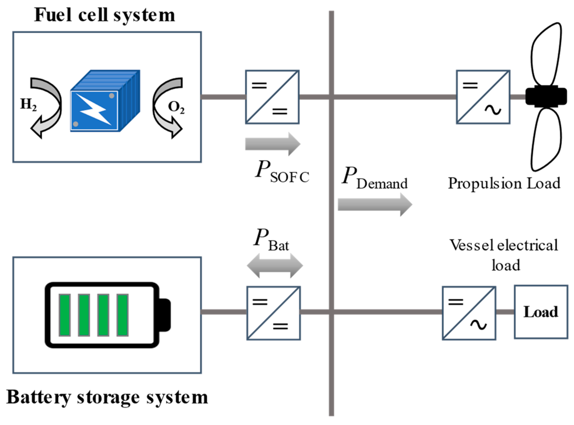
2.1. Hybrid Propulsion System
- ▪
- PSOFC,min = 0 W
- ▪
- PSOFC,max = 45 MW
- ▪
- EBat = 5 MWh
- ▪
- PBat,max = 10 MW (or 2C)
2.2. Hydrodynamic Aspects
2.3. Losses in the Drive Train
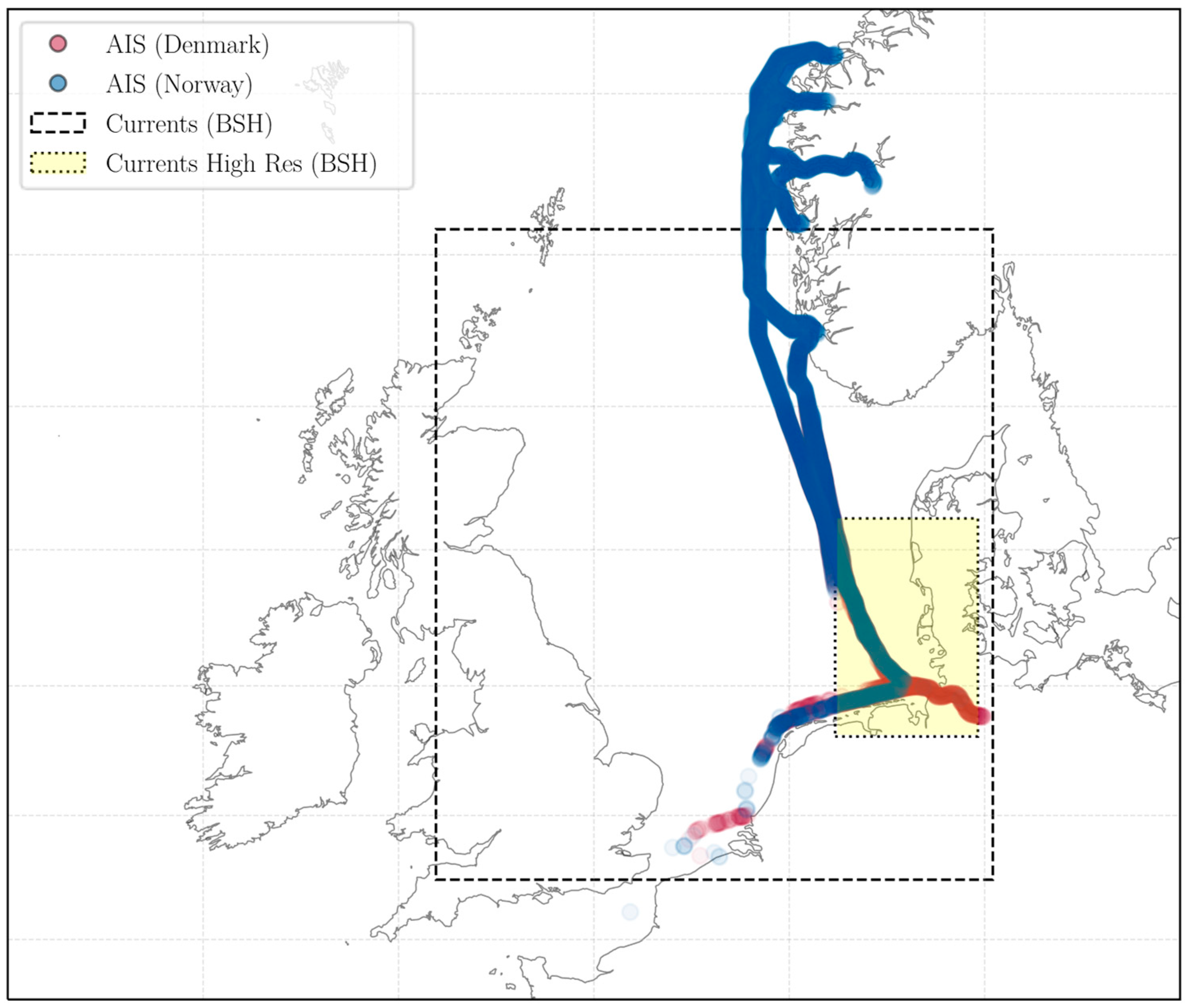
2.4. Data Collection
2.5. Processing of the Collected Data
3. Simulation of Propulsion Components and Energy Management Development
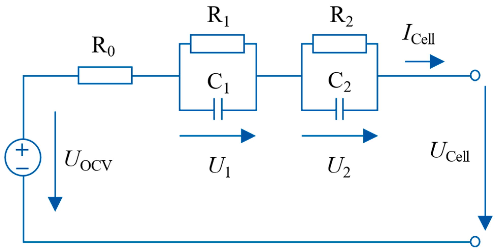
3.1. Modeling of the Battery
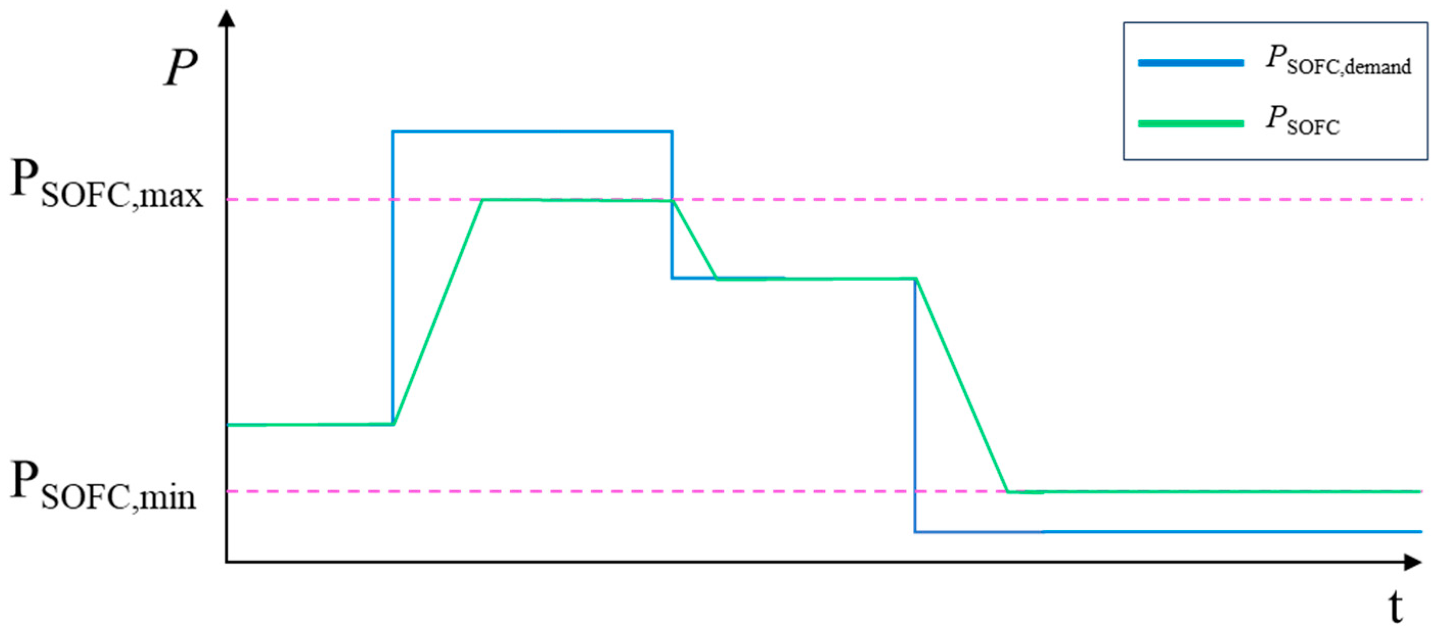
3.2. Modeling of the Fuel Cell
Evaluation Criterion for the Attenuation of the Power Output Behavior of the SOFC
3.3. Rule-Based Energy Management Method
3.4. Development of a Load Demand Estimator
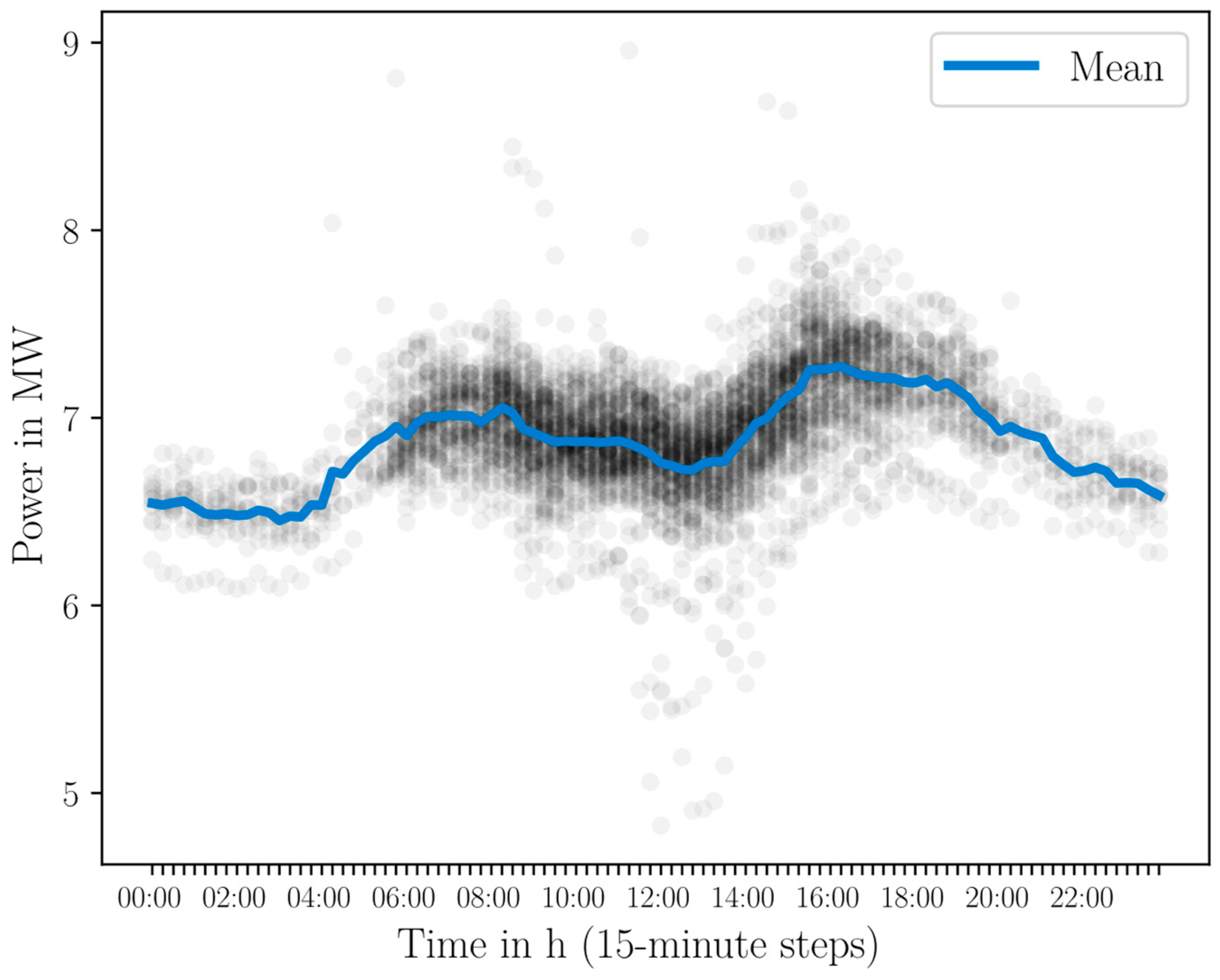
3.4.1. Empirical Analysis of the Base Load
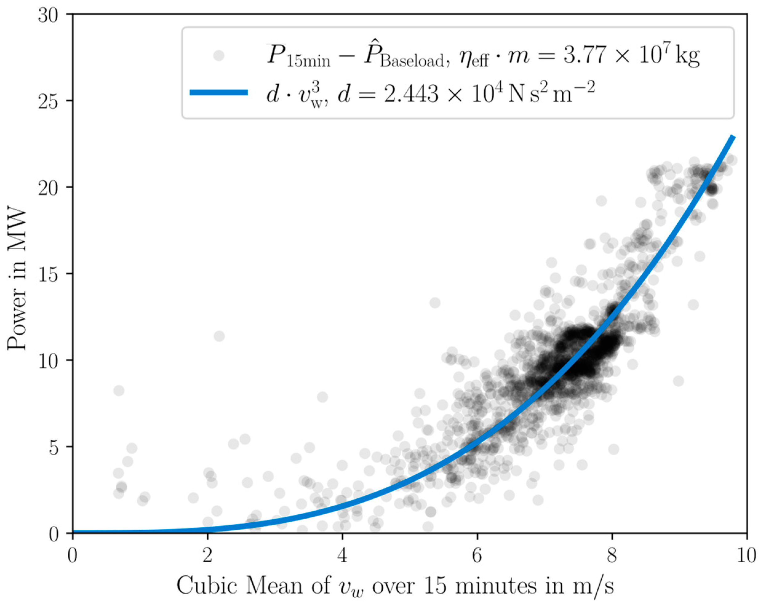
3.4.2. Analysis of the Propulsion Load
4. Results
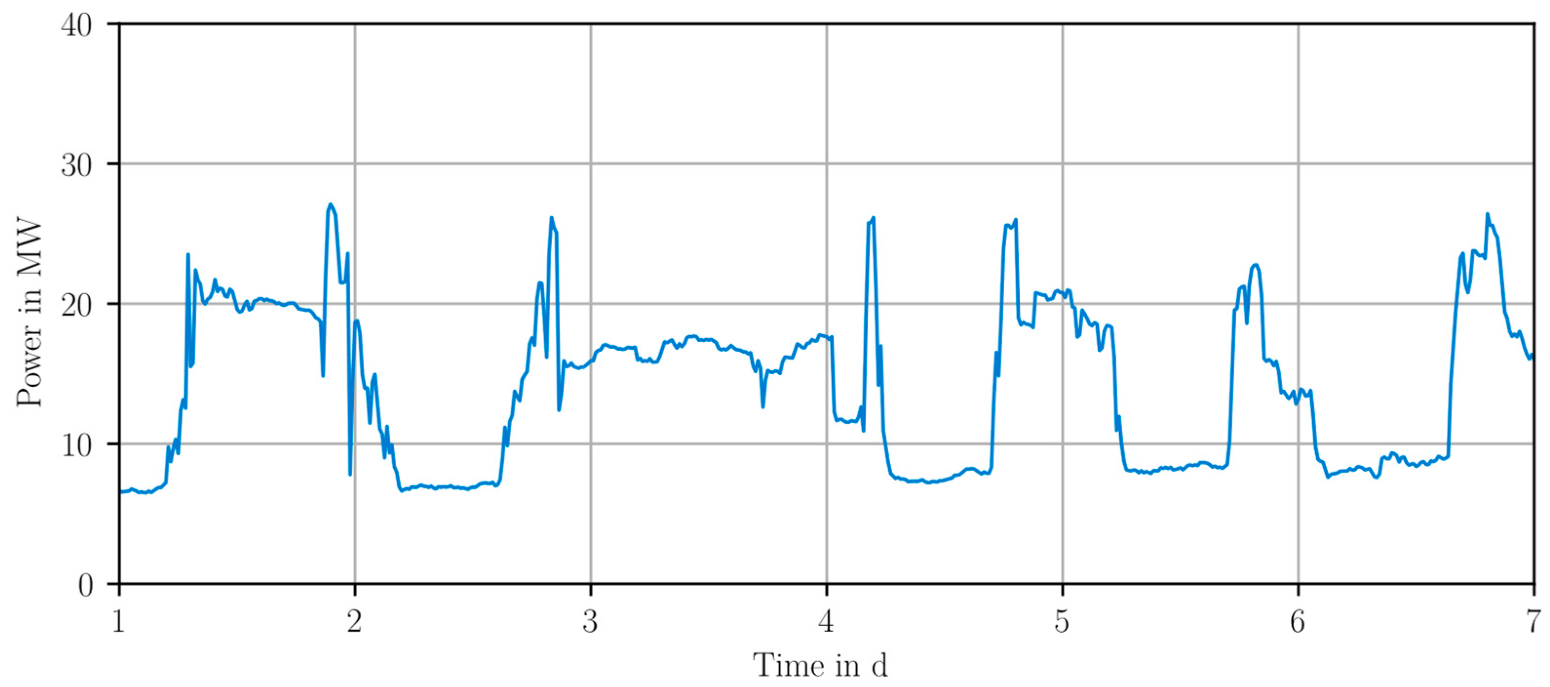
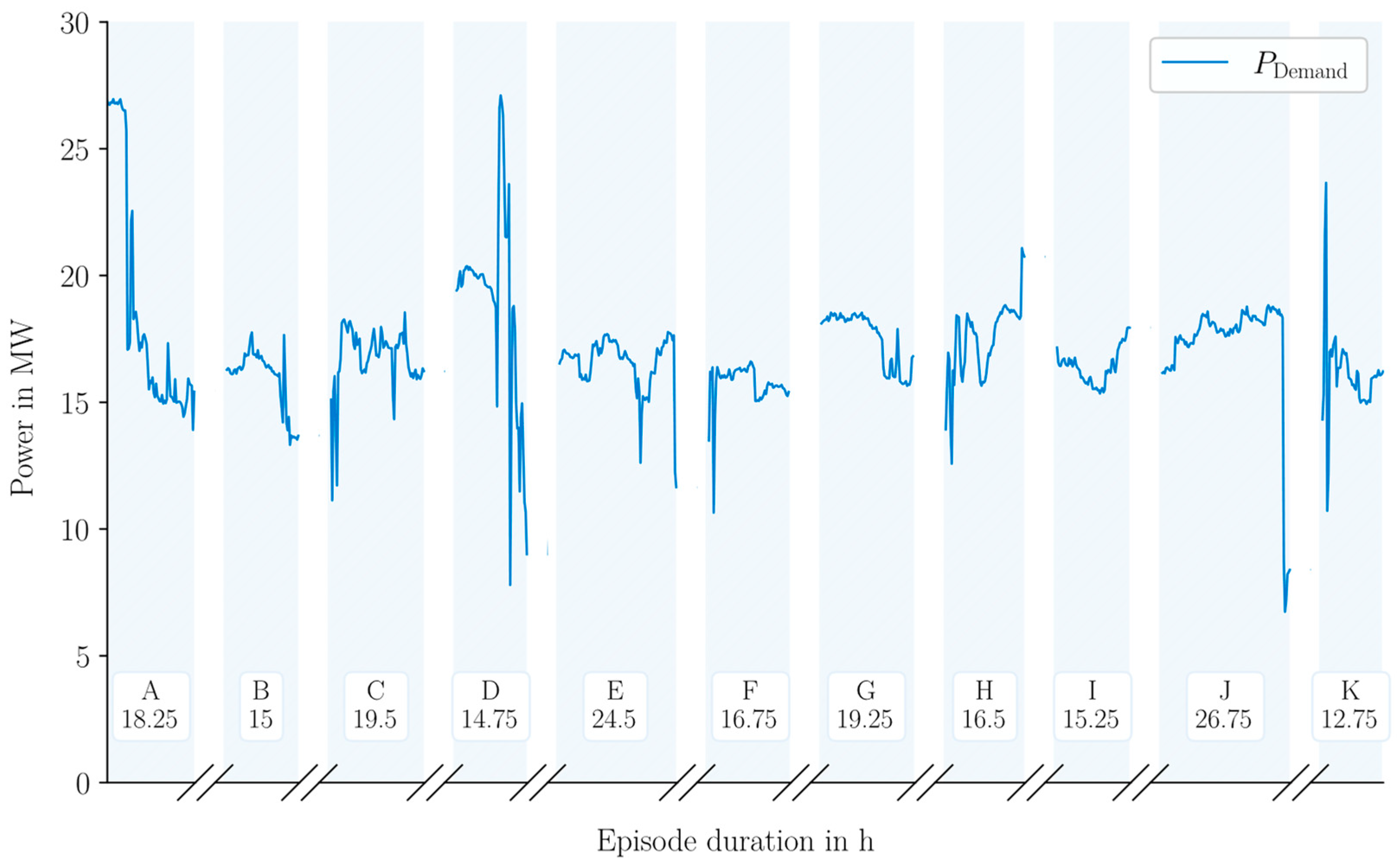
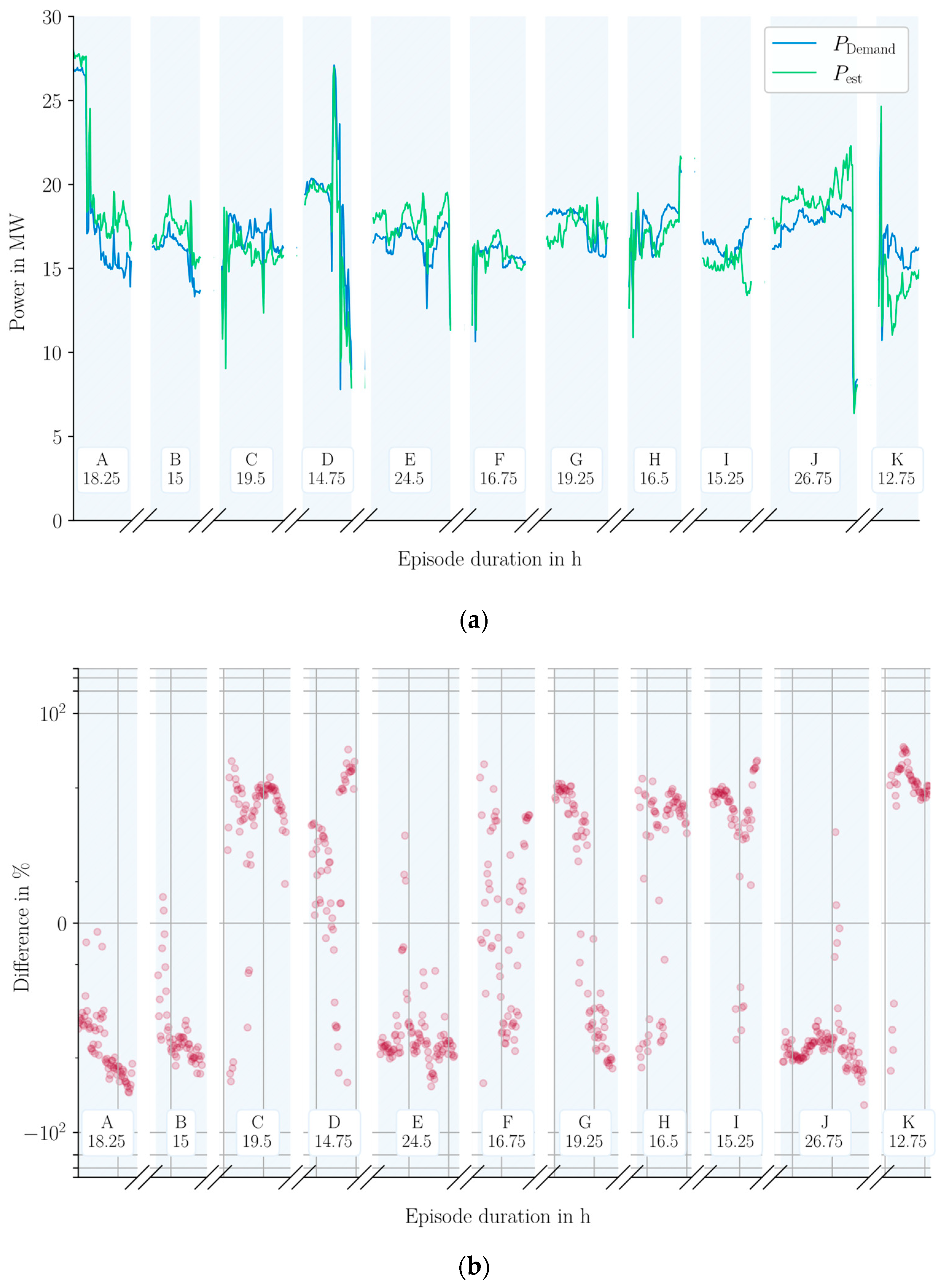
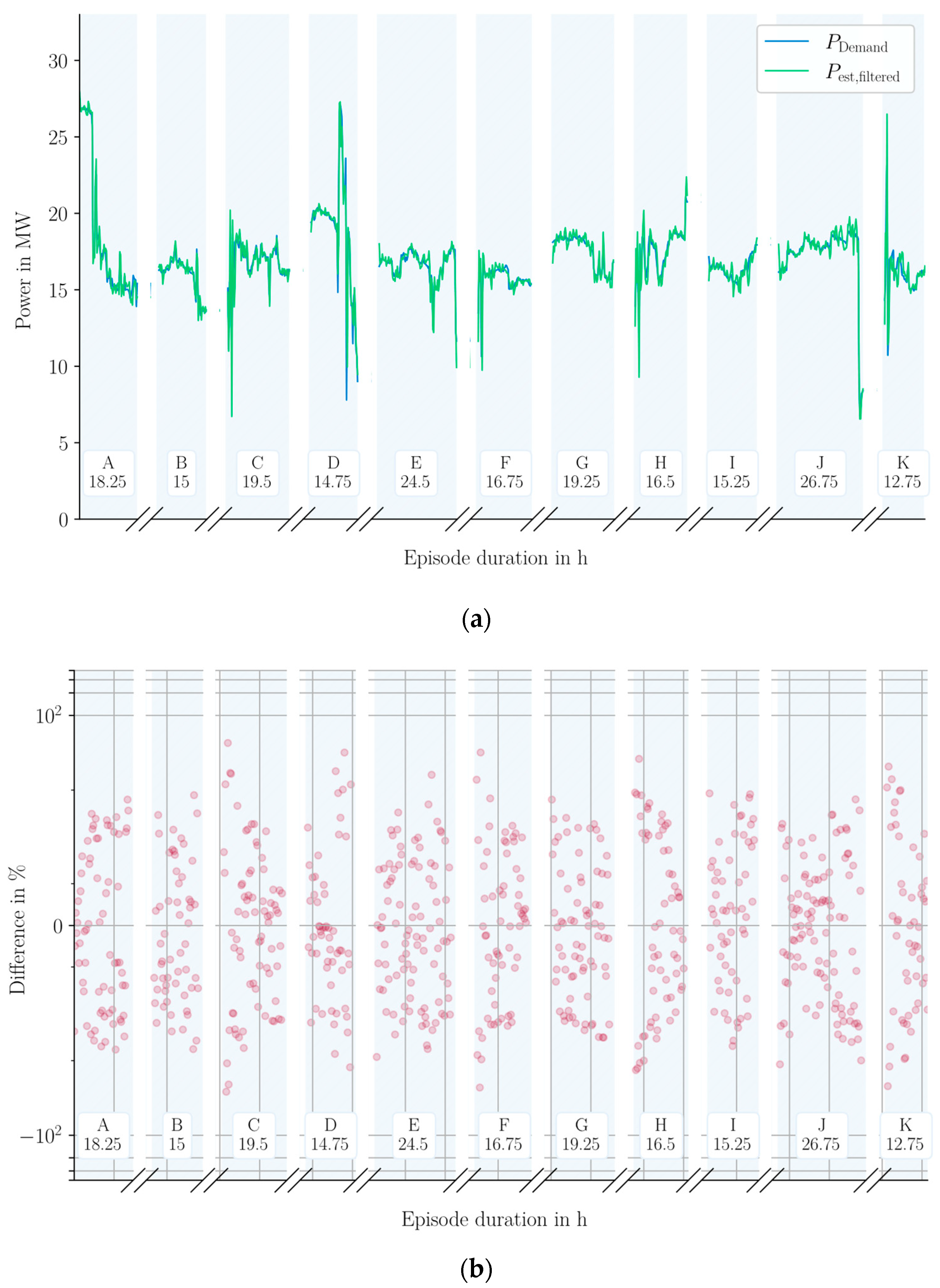
4.1. Estimation of the Total Load and Power Requirement of a Vessel
4.2. Look-Ahead Energy Management Method
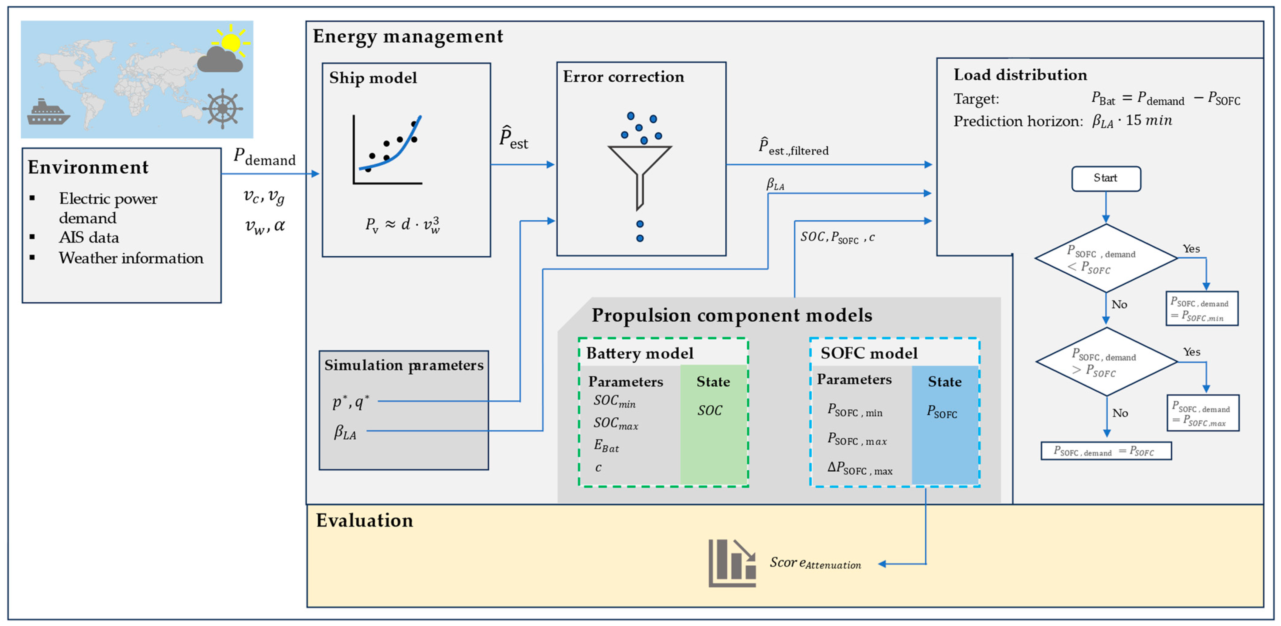
4.2.1. Definition of the Energy Management Method
- The SOC should be kept over time in a pre-definable operational range to keep the battery in a safe operational window and avoid degradation due to a higher depth of discharge [41].
- The SOFC should change its output power only if it is foreseeable that a deviating average power is to be provided by the propulsion system.
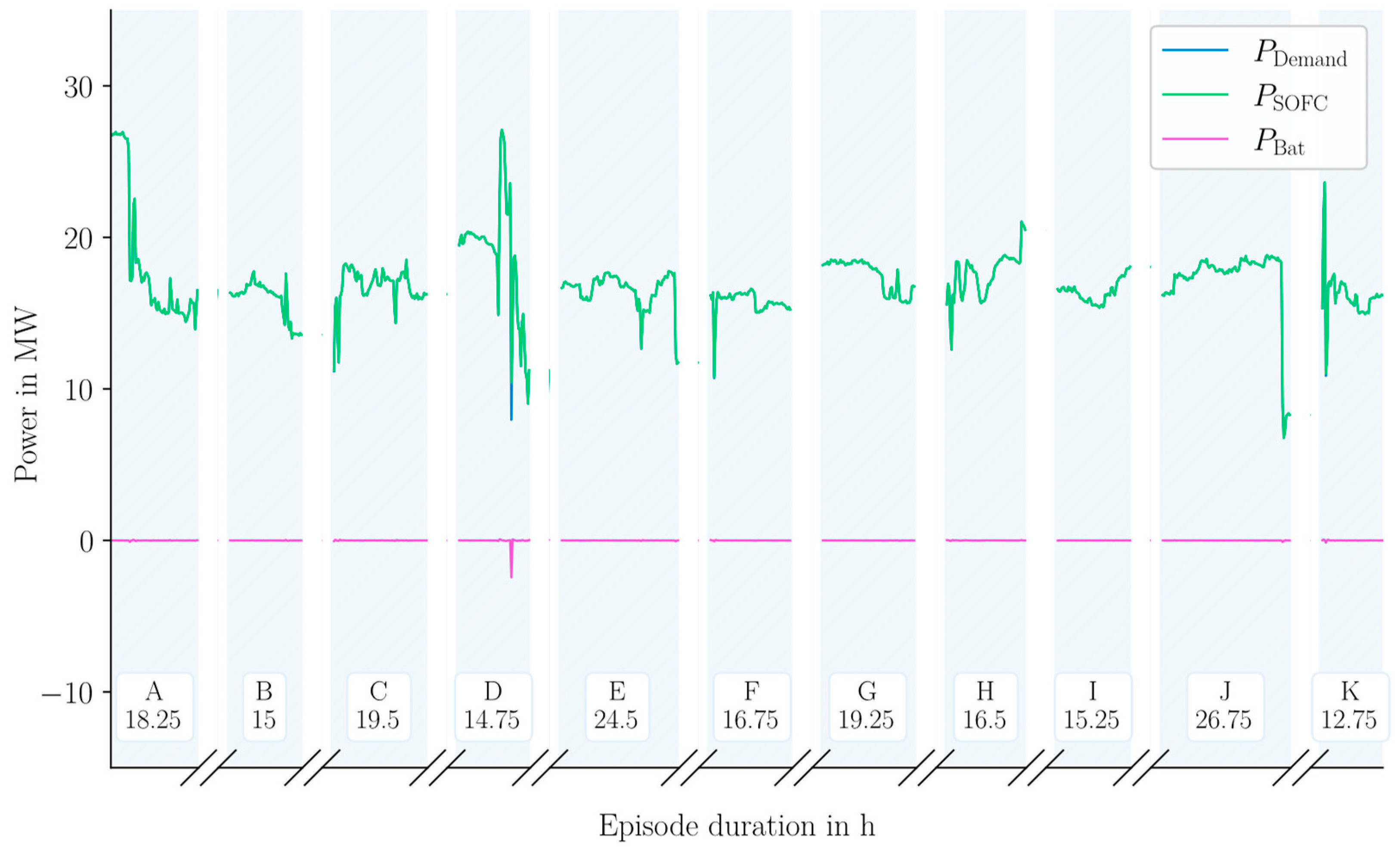
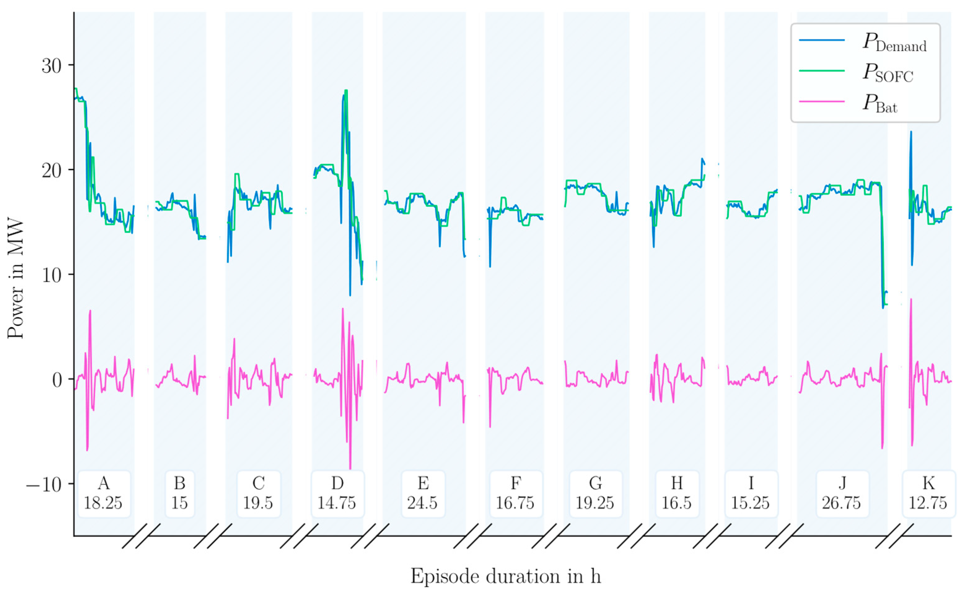
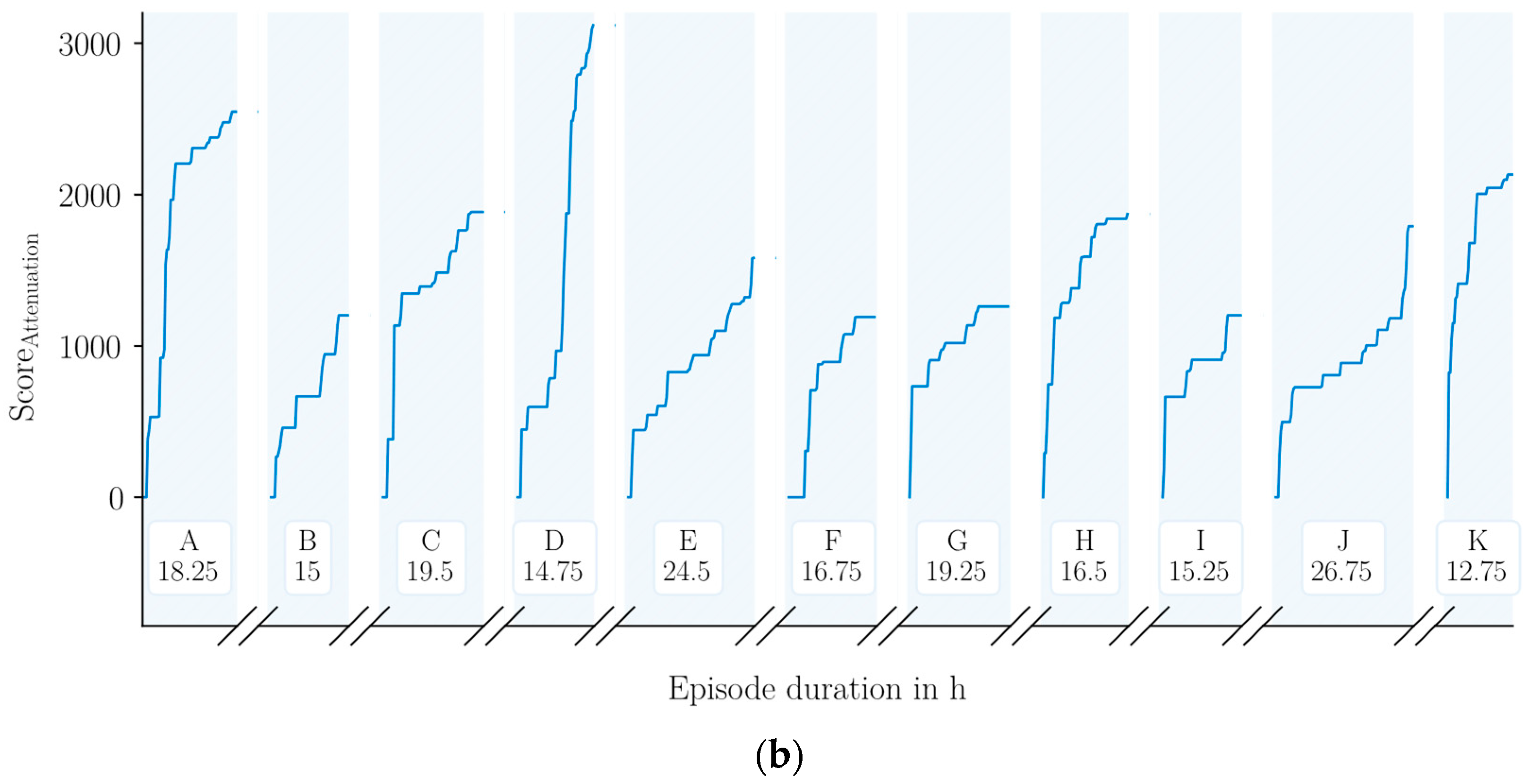
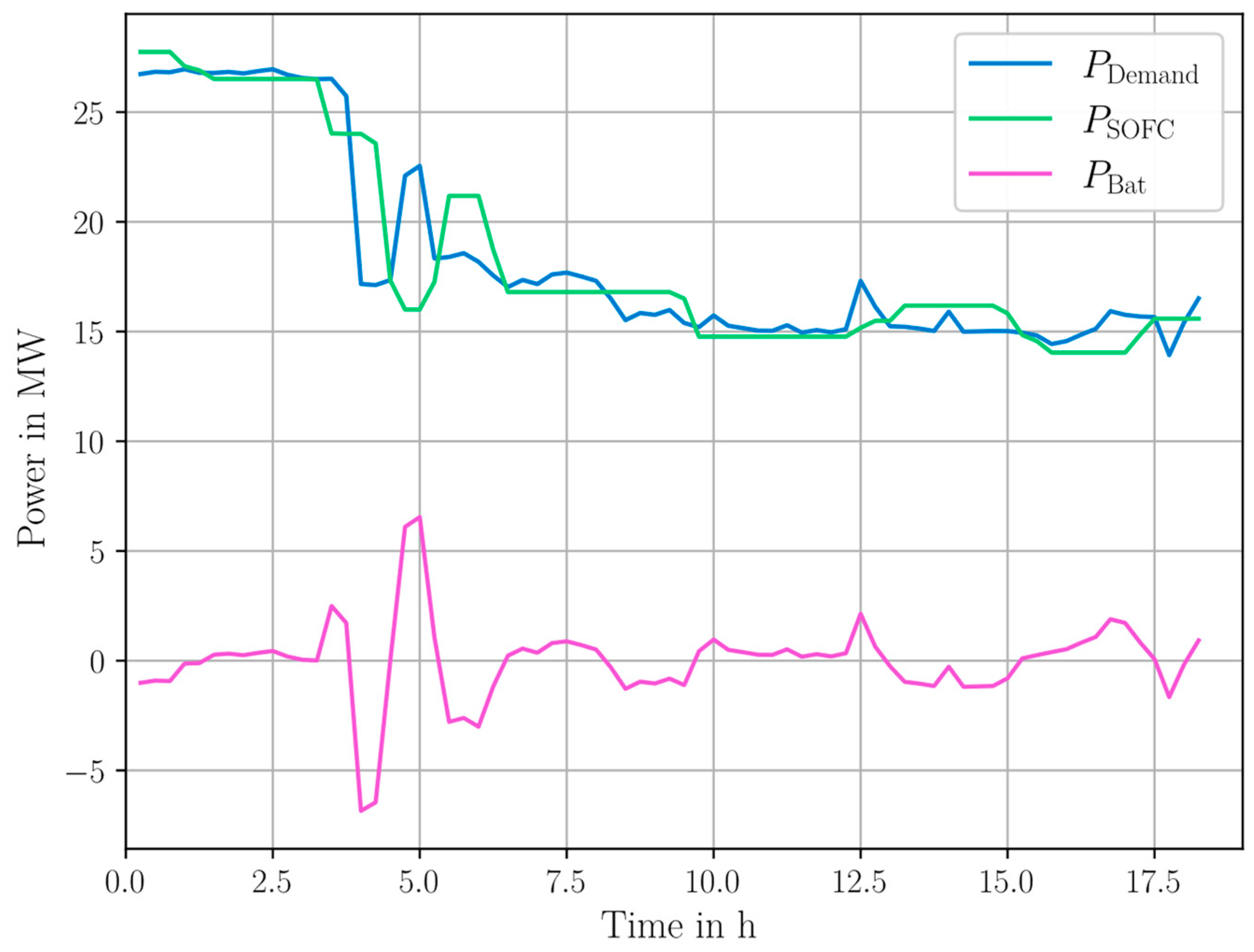
4.2.2. Simulation of the EMS and Performance Check
5. Discussion
Outlook and Future Work
Author Contributions
Funding
Data Availability Statement
Conflicts of Interest
Nomenclature
| Abbreviations | |
| AIS | Automatic Identification System |
| ECM | Equivalent circuit model |
| EMS | Energy management system |
| GPS | Global Positioning System |
| ICE | Internal combustion engine |
| LIB | Lithium-ion battery |
| SOC | State of charge |
| SOFC | Solid oxide fuel cell |
| Parameters | |
| Angle of the velocity vector | |
| Configurable factor to determine the prediction horizon | |
| Charge or discharge factor of the battery | |
| Battery capacity | |
| Cubic coefficient for the calculation of the relation between measured power demand and speed of the vessel | |
| EBat | Capacity or maximum energy content of the battery |
| Mass of the vessel | |
| Coulomb efficiency | |
| Drive train efficiency | |
| Arithmetic mean of load demand in harbor mode for 15 min time resolution | |
| PBat(t) | Power provided or drawn by the battery at time t |
| PBat,max | Maximum power out-/input of the battery |
| Absolute in- or output power of the battery | |
| = | Mean estimated power demand for given velocities |
| Filtered estimated power demand | |
| Change in power after a time step required for propulsion | |
| PSOFC(t) | Actual power provided by the fuel cell at time t |
| PSOFC,demand(t) | Power demand applied to the fuel cell at time t |
| PSOFC,min | The minimum power output of the fuel cell; 0 W in the presented simulation |
| Rate of change of the output power of the solid oxide fuel cell | |
| PSOFC,max | The maximum power output of the fuel cell |
| SOCmin | Lower SOC boundary for the simulation |
| SOCmax | Upper SOC boundary for the simulation |
| Battery cell voltage | |
| Battery cell open circuit voltage | |
| Velocity of ocean currents | |
| Velocity over ground | |
| Velocity through water |
References
- United Nations Conference on Trade and Development. 50 Years of Review of Maritime Transport, 1968–2018: Reflecting on the Past, Exploring the Future; No. UNCTAD/DTL/2018/1; United Nations Conference on Trade and Development: Geneva, Switzerland, 2018. [Google Scholar]
- International Maritime Organization. Fourth IMO GHG Study 2020. 2021. Available online: https://wwwcdn.imo.org/localresources/en/OurWork/Environment/Documents/Fourth%20IMO%20GHG%20Study%202020%20-%20Full%20report%20and%20annexes.pdf (accessed on 31 October 2023).
- Mallouppas, G.; Yfantis, E.A. Decarbonization in Shipping Industry: A Review of Research, Technology Development, and Innovation Proposals. J. Mar. Sci. Eng. 2021, 9, 415. [Google Scholar] [CrossRef]
- Chin, C.S.; Tan, Y.-J.; Kumar, M.V. Study of Hybrid Propulsion Systems for Lower Emissions and Fuel Saving on Merchant Ship during Voyage. J. Mar. Sci. Eng. 2022, 10, 393. [Google Scholar] [CrossRef]
- Kolodziejski, M.; Michalska-Pozoga, I. Battery Energy Storage Systems in Ships’ Hybrid/Electric Propulsion Systems. Energies 2023, 16, 1122. [Google Scholar] [CrossRef]
- Kersey, J.; Popovich, N.D.; Phadke, A.A. Rapid battery cost declines accelerate the prospects of all-electric interregional container shipping. Nat. Energy 2022, 7, 664–674. [Google Scholar] [CrossRef]
- Dokiya, M. SOFC system and technology. Solid. State Ion. 2002, 152–153, 383–392. [Google Scholar] [CrossRef]
- Fang, Q.; Blum, L.; Stolten, D. Electrochemical Performance and Degradation Analysis of an SOFC Short Stack Following Operation of More than 100,000 Hours. J. Electrochem. Soc. 2019, 166, F1320–F1325. [Google Scholar] [CrossRef]
- Machaj, K.; Kupecki, J.; Malecha, Z.; Morawski, A.W.; Skrzypkiewicz, M.; Stanclik, M.; Chorowski, M. Ammonia as a potential marine fuel: A review. Energy Strategy Rev. 2022, 44, 100926. [Google Scholar] [CrossRef]
- Lin, Y.; Zhan, Z.; Liu, J.; Barnett, S. Direct operation of solid oxide fuel cells with methane fuel. Solid. State Ion. 2005, 176, 1827–1835. [Google Scholar] [CrossRef]
- Fan, L.; Tu, Z.; Chan, S.H. Recent development of hydrogen and fuel cell technologies: A review. Energy Rep. 2021, 7, 8421–8446. [Google Scholar] [CrossRef]
- Obara, S. Dynamic-characteristics analysis of an independent microgrid consisting of a SOFC triple combined cycle power generation system and large-scale photovoltaics. Appl. Energy 2015, 141, 19–31. [Google Scholar] [CrossRef]
- Shen, M. Solid oxide fuel cell-lithium battery hybrid power generation system energy management: A review. Int. J. Hydrogen Energy 2021, 46, 32974–32994. [Google Scholar] [CrossRef]
- Zhang, L.; Xie, H.; Niu, Q.; Wang, F.; Xie, C.; Wang, G. Optimization of energy management in hybrid SOFC-based DC microgrid considering high efficiency and operating safety when external load power goes up. Sustain. Energy Fuels 2023, 7, 1433–1446. [Google Scholar] [CrossRef]
- Wu, Z.; Zhu, P.; Yao, J.; Tan, P.; Xu, H.; Chen, B.; Yang, F.; Zhang, Z.; Porpatham, E.; Ni, M. Dynamic modeling and operation strategy of natural gas fueled SOFC-Engine hybrid power system with hydrogen addition by metal hydride for vehicle applications. ETransportation 2020, 5, 100074. [Google Scholar] [CrossRef]
- Wang, X.; Zhu, J.; Han, M. Industrial Development Status and Prospects of the Marine Fuel Cell: A Review. J. Mar. Sci. Eng. 2023, 11, 238. [Google Scholar] [CrossRef]
- Valadez Huerta, G.; Álvarez Jordán, J.; Marquardt, T.; Dragon, M.; Leites, K.; Kabelac, S. Exergy analysis of the diesel pre-reforming SOFC-system with anode off-gas recycling in the SchIBZ project. Part II: System exergetic evaluation. Int. J. Hydrogen Energy 2019, 44, 10916–10924. [Google Scholar] [CrossRef]
- van Veldhuizen, B.N.; van Biert, L.; Amladi, A.; Woudstra, T.; Visser, K.; Aravind, P.V. The effects of fuel type and cathode off-gas recirculation on combined heat and power generation of marine SOFC systems. Energy Convers. Manag. 2023, 276, 116498. [Google Scholar] [CrossRef]
- Kistner, L.; Schubert, F.L.; Minke, C.; Bensmann, A.; Hanke-Rauschenbach, R. Techno-economic and Environmental Comparison of Internal Combustion Engines and Solid Oxide Fuel Cells for Ship Applications. J. Power Sources 2021, 508, 230328. [Google Scholar] [CrossRef]
- van Biert, L.; Godjevac, M.; Visser, K.; Aravind, P.V. A review of fuel cell systems for maritime applications. J. Power Sources 2016, 327, 345–364. [Google Scholar] [CrossRef]
- Dinu, O.; Ilie, A.M. Maritime vessel obsolescence, life cycle cost and design service life. IOP Conf. Ser. Mater. Sci. Eng. 2015, 95, 12067. [Google Scholar] [CrossRef]
- Khan, M.Z.; Mehran, M.T.; Song, R.-H.; Lee, S.-B.; Lim, T.-H. Effects of applied current density and thermal cycling on the degradation of a solid oxide fuel cell cathode. Int. J. Hydrogen Energy 2018, 43, 12346–12357. [Google Scholar] [CrossRef]
- Hanasaki, M.; Uryu, C.; Daio, T.; Kawabata, T.; Tachikawa, Y.; Lyth, S.M.; Shiratori, Y.; Taniguchi, S.; Sasaki, K. SOFC Durability against Standby and Shutdown Cycling. J. Electrochem. Soc. 2014, 161, F850–F860. [Google Scholar] [CrossRef]
- Ma, Z.; Chen, H.; Han, J.; Chen, Y.; Kuang, J.; Charpentier, J.-F.; Aϊt-Ahmed, N.; Benbouzid, M. Optimal SOC Control and Rule-Based Energy Management Strategy for Fuel-Cell-Based Hybrid Vessel including Batteries and Supercapacitors. J. MAR. SCI. ENG. 2023, 11, 398. [Google Scholar] [CrossRef]
- Dinh, T.Q.; Bui, T.M.; Marco, J.; Watts, C.; Yoon, J.I. Optimal Energy Management for Hybrid Electric Dynamic Positioning Vessels. IFAC-Pap. 2018, 51, 98–103. [Google Scholar] [CrossRef]
- Bui, T.M.N.; Dinh, T.Q.; Marco, J.; Watts, C. Development and Real-Time Performance Evaluation of Energy Management Strategy for a Dynamic Positioning Hybrid Electric Marine Vessel. Electronics 2021, 10, 1280. [Google Scholar] [CrossRef]
- Bassam, A.M.; Phillips, A.B.; Turnock, S.R.; Wilson, P.A. Development of a multi-scheme energy management strategy for a hybrid fuel cell driven passenger ship. Int. J. Hydrogen Energy 2017, 42, 623–635. [Google Scholar] [CrossRef]
- Kistner, L.; Bensmann, A.; Hanke-Rauschenbach, R. Optimal Design of Power Gradient Limited Solid Oxide Fuel Cell Systems with Hybrid Storage Support for Ship Applications. Energy Convers. Manag. 2021, 243, 114396. [Google Scholar] [CrossRef]
- Li, J.; Herdem, M.S.; Nathwani, J.; Wen, J.Z. Methods and applications for Artificial Intelligence, Big Data, Internet of Things, and Blockchain in smart energy management. Energy AI 2023, 11, 100208. [Google Scholar] [CrossRef]
- Haseltalab, A.; Negenborn, R.R. Model predictive maneuvering control and energy management for all-electric autonomous ships. Appl. Energy 2019, 251, 113308. [Google Scholar] [CrossRef]
- International Maritime Organization. Resolution A. 1106(29) Revised Guidelines for the Onboard Operational Use of Shipborne Automatic Identification Systems (AIS); IMO: London, UK, 2015. [Google Scholar]
- Lee, E.; Mokashi, A.J.; Moon, S.Y.; Kim, G. The Maturity of Automatic Identification Systems (AIS) and Its Implications for Innovation. J. Mar. Sci. Eng. 2019, 7, 287. [Google Scholar] [CrossRef]
- Kim, S.-H.; Roh, M.-I.; Oh, M.-J.; Park, S.-W.; Kim, I.-I. Estimation of ship operational efficiency from AIS data using big data technology. Int. J. Nav. Archit. Ocean. Eng. 2020, 12, 440–454. [Google Scholar] [CrossRef]
- Hoerner, S.F. Fluid-Dynamic Drag; Midland Park, NJ, USA, 1965; Available online: https://ia600707.us.archive.org/13/items/FluidDynamicDragHoerner1965/Fluid-dynamic_drag__Hoerner__1965_text.pdf.
- Sündermann, J.; Pohlmann, T. A brief analysis of North Sea physics. Oceanologia 2011, 53, 663–689. [Google Scholar] [CrossRef]
- Tadros, M.; Ventura, M.; Guedes Soares, C. Design of Propeller Series Optimizing Fuel Consumption and Propeller Efficiency. J. Mar. Sci. Eng. 2021, 9, 1226. [Google Scholar] [CrossRef]
- Ghimire, P.; Park, D.; Zadeh, M.K.; Thorstensen, J.; Pedersen, E. Shipboard Electric Power Conversion: System Architecture, Applications, Control, and Challenges [Technology Leaders]. IEEE Electrific. Mag. 2019, 7, 6–20. [Google Scholar] [CrossRef]
- Sakile, R.; Sinha, U.K. Estimation of lithium-ion battery state of charge for electric vehicles using a nonlinear state observer. Energy Storage 2022, 4, e290. [Google Scholar] [CrossRef]
- Institute for Power Electronics and Electrical Drives. ISEA Framework. Available online: https://git.rwth-aachen.de/isea/framework (accessed on 26 July 2023).
- Waag, W.; Käbitz, S.; Sauer, D.U. Experimental investigation of the lithium-ion battery impedance characteristic at various conditions and aging states and its influence on the application. Appl. Energy 2013, 102, 885–897. [Google Scholar] [CrossRef]
- Ecker, M.; Nieto, N.; Käbitz, S.; Schmalstieg, J.; Blanke, H.; Warnecke, A.; Sauer, D.U. Calendar and cycle life study of Li(NiMnCo)O2-based 18650 lithium-ion batteries. J. Power Sources 2014, 248, 839–851. [Google Scholar] [CrossRef]
- Whiston, M.M.; Azevedo, I.M.; Litster, S.; Samaras, C.; Whitefoot, K.S.; Whitacre, J.F. Meeting U.S. Solid Oxide Fuel Cell Targets. Joule 2019, 3, 2060–2065. [Google Scholar] [CrossRef]


| Specification | Value | Details |
|---|---|---|
| Ship size | 127,000 GRT | 1 gross register tonnage (GRT) = 100 cubic feet ≈ 2.83 m3 |
| Ship length | 300 m | |
| Maximum electrical power demand | 46.8 MW | Sum of propulsion power demand and hotel power demand |
| Draft (hull) | 8.1 m | |
| Maximum speed | 22 knots | 22 knots = 40.74 km/h |
| Source | Data Type | Details |
|---|---|---|
| Federal Maritime and Hydrographic Agency of Germany (German: Bundesamt für Seeschifffahrt und Hydrographie, short BSH) | Current data and AIS | Current data for the North Sea and in somewhat higher spatial resolution for the German Bight from observations and estimates based on physical models |
| Danish Maritime Authority | AIS | Data from all ships that have sailed in waters surrounding Denmark |
| Norwegian Coastal Administration | AIS | Data from ships worldwide with varying resolution |
| United Nations | AIS | Data from ships worldwide with varying resolution |
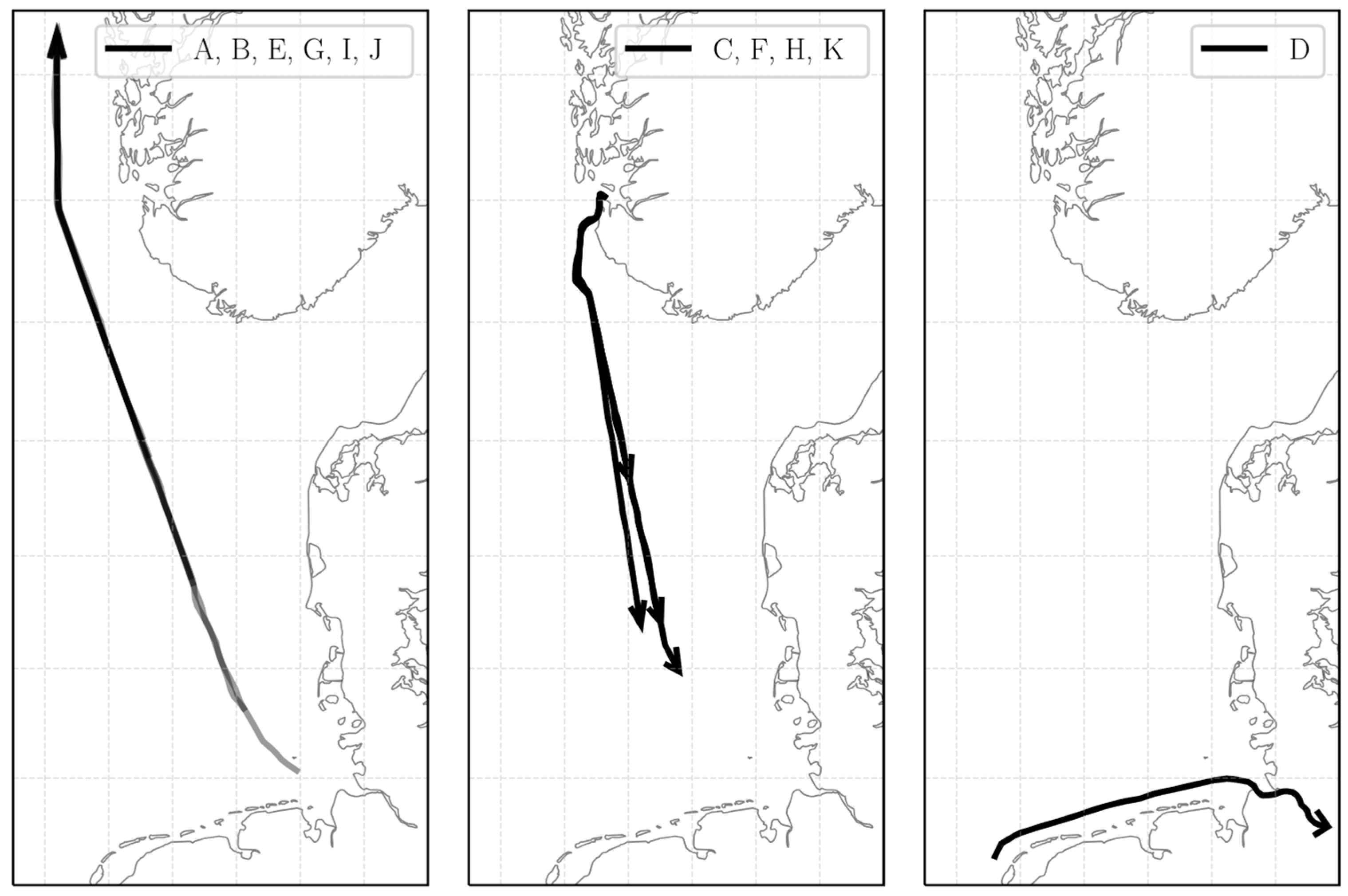
| Name | Group | Start Time (UTC) | End Time (UTC) | Duration in hh:mm | ||
|---|---|---|---|---|---|---|
| A | I | May 19 | 08:30 | May 20 | 02:45 | 18:15 |
| B | I | Jun 09 | 11:15 | Jun 10 | 02:15 | 15:00 |
| C | II | Jun 13 | 20:30 | Jun 14 | 16:00 | 19:30 |
| D | III | Jun 28 | 13:30 | Jun 29 | 04:15 | 14:45 |
| E | I | Jun 30 | 01:45 | Jul 01 | 02:15 | 24:30 |
| F | II | Jul 04 | 20:30 | Jul 05 | 13:15 | 16:45 |
| G | I | Jul 21 | 07:15 | Jul 22 | 02:30 | 19:15 |
| H | II | Jul 25 | 20:30 | Jul 26 | 13:00 | 16:30 |
| I | I | Aug 11 | 11:30 | Aug 12 | 02:45 | 15:15 |
| J | I | Sep 21 | 22:45 | Sep 23 | 01:30 | 26:45 |
| K | II | Sep 26 | 16:00 | Sep 27 | 04:45 | 12:45 |
| Description | Value |
|---|---|
| CCell | 64 Ah |
| Nominal cell voltage | 3.7 V |
| Cell voltage range | 3.0–4.2 V |
| R0 | 0.75 × 10⁻³ … 1.70 × 10⁻³ Ω |
| τ1 = R1∙C1 | 13.04 … 100.00 s |
| τ2 = R2∙C2 | 385.54 … 1.00 × 10⁴ s |
| Episode | ScoreAttenuation | |
|---|---|---|
| Look-Ahead | Rule-Based EMS | |
| A | 2546 | 3113 |
| B | 1202 | 2206 |
| C | 1886 | 3028 |
| D | 3119 | 4529 |
| E | 1582 | 2173 |
| F | 1191 | 2336 |
| G | 1261 | 1692 |
| H | 1872 | 2793 |
| I | 1202 | 1626 |
| J | 1791 | 2036 |
| K | 2132 | 3579 |
Disclaimer/Publisher’s Note: The statements, opinions and data contained in all publications are solely those of the individual author(s) and contributor(s) and not of MDPI and/or the editor(s). MDPI and/or the editor(s) disclaim responsibility for any injury to people or property resulting from any ideas, methods, instructions or products referred to in the content. |
© 2023 by the authors. Licensee MDPI, Basel, Switzerland. This article is an open access article distributed under the terms and conditions of the Creative Commons Attribution (CC BY) license (https://creativecommons.org/licenses/by/4.0/).
Share and Cite
Ünlübayir, C.; Mierendorff, U.H.; Börner, M.F.; Quade, K.L.; Blömeke, A.; Ringbeck, F.; Sauer, D.U. A Data-Driven Approach to Ship Energy Management: Incorporating Automated Tracking System Data and Weather Information. J. Mar. Sci. Eng. 2023, 11, 2259. https://doi.org/10.3390/jmse11122259
Ünlübayir C, Mierendorff UH, Börner MF, Quade KL, Blömeke A, Ringbeck F, Sauer DU. A Data-Driven Approach to Ship Energy Management: Incorporating Automated Tracking System Data and Weather Information. Journal of Marine Science and Engineering. 2023; 11(12):2259. https://doi.org/10.3390/jmse11122259
Chicago/Turabian StyleÜnlübayir, Cem, Ulrich Hermann Mierendorff, Martin Florian Börner, Katharina Lilith Quade, Alexander Blömeke, Florian Ringbeck, and Dirk Uwe Sauer. 2023. "A Data-Driven Approach to Ship Energy Management: Incorporating Automated Tracking System Data and Weather Information" Journal of Marine Science and Engineering 11, no. 12: 2259. https://doi.org/10.3390/jmse11122259
APA StyleÜnlübayir, C., Mierendorff, U. H., Börner, M. F., Quade, K. L., Blömeke, A., Ringbeck, F., & Sauer, D. U. (2023). A Data-Driven Approach to Ship Energy Management: Incorporating Automated Tracking System Data and Weather Information. Journal of Marine Science and Engineering, 11(12), 2259. https://doi.org/10.3390/jmse11122259