AUV Collision Avoidance Planning Method Based on Deep Deterministic Policy Gradient

Abstract

Collision avoidance planning has always been a hot and important issue in the field of unmanned aircraft research. In this article, we describe an online collision avoidance planning algorithm for autonomous underwater vehicle (AUV) autonomous navigation, which relies on its own active sonar sensor to detect obstacles. The improved particle swarm optimization (I-PSO) algorithm is used to complete the path planning of the AUV under the known environment, and we use it as a benchmark to improve the fitness function and inertia weight of the algorithm. Traditional path-planning algorithms rely on accurate environment maps, where re-adapting the generated path can be highly demanding in terms of computational cost. We propose a deep reinforcement learning (DRL) algorithm based on collision avoidance tasks. The algorithm discussed in this paper takes into account the relative position of the target point and the rate of heading change from the previous timestep. Its reward function considers the target point, running time and turning angle at the same time. Compared with the LSTM structure, the Gated Recurrent Unit (GRU) network has fewer parameters, which helps to save training time. A series of simulation results show that the proposed deep deterministic policy gradient (DDPG) algorithm can obtain excellent results in simple and complex environments.

1. Introduction

As robotic systems become more reliable and powerful, the burden of performing difficult or tedious tasks in dangerous and inaccessible marine environments is shifting from humans towards unmanned platforms, such as marine resource exploration, aircraft wreckage search, intelligence gathering, searching an area for potential mine-like objects, etc. Considering the communication limitations and operational difficulties in large-scale underwater areas, it is clear that autonomous underwater vehicles (AUVs) require effective and reliable path planning to successfully complete their missions.

Autonomous navigation is a classic research field of robotics, which has produced a variety of methods, as described in detail in the literature. Local collision avoidance planning when there are obstacles often relies on local smoothing methods, such as splines. The author uses a variant of A* to find a feasible trajectory point and applies the conjugate gradient method to realize the collision avoidance plan of autonomous vehicles [1]. The work in [2] considers two different types of unmanned vehicles that explore the plane using A* search and the genetic algorithm (GA) that independently solves multiple optimization goals. The author proposes a combination of discrete search and sampling-based motion. The AUV planner can achieve multi-objective information collection and dynamic obstacle avoidance [3]. The authors propose a gaussian random paths motion planner (GRPMP) to generate a set of discretized smooth random path nodes that are sparse and use the GRPMP sampler to quickly select smooth random paths with the lowest-cost collision-free high-quality paths [4]. The authors propose a parallel elite genetic algorithm (PEGA) combined with the cubic B-spline technique for the global path planning of autonomous mobile robots navigating in structured environments [5]. The performance of the above algorithms is highly sensitive to the space complexity of the problem being solved. As the number of individuals increases, the time consumption of the algorithm grows exponentially, and it is prone to converging to local optima.

The author proposes a hybrid algorithm of the particle swarm optimization (PSO) algorithm and legendre pseudo spectral method (LPM), which is designed for AUVs to achieve time-optimal collision-free path planning in static and dynamic environments [6]. The author proposes an online planner based on particle swarm optimization (QPSO), which is used to deal with the problem of path planning in the dynamic environment of AUVs [7,8]. In addition to considering the optimal path, the author also uses the membership function to evaluate the degree of danger of the path to realize the path planning of the robot in an unknown environment [9]. When the AUV is operating in an unknown or partially known dynamic obstacle environment, local re-planning due to continuous changes in the environment should be performed online, which increases the uncertainty of the path-planning problem and cannot always guarantee the best solution.

In a continuous large-scale space, it is difficult to perform obstacle avoidance using only reinforcement learning (RL), as this requires long-term learning and is relatively inefficient. The continuity of the state and action spaces leads to the so-called dimensionality disaster, and traditional RL cannot be applied in any effective form. Although dynamic programming (DP) can be applied to continuous problems, accurate solutions can only be obtained for special cases. Many scholars combine RL with fuzzy logic, supervised learning and transfer learning to realize the autonomous planning of robots [10,11,12,13]. For example, [10] proposes the use of RL to teach collision avoidance behavior and goal-seeking behavior rules, thus allowing the correct course of action to be determined. The advantage of this approach is that it requires simple evaluation data rather than thousands of input–output training data. In [11], a neural fuzzy system with a hybrid learning algorithm is proposed, in which supervised learning is used to determine the input and output membership functions, and an RL algorithm is used to finetune the output membership functions. The main advantage of this hybrid approach is that, with the help of supervised learning, the search space for RL is reduced and the learning process is accelerated, eventually leading to better fuzzy logic rules. Meng [12] describes the use of a fuzzy actor–critic learning algorithm that enables a robot to readapt to the new environment without human intervention. The generalized dynamic fuzzy neural network is trained by supervised learning to approximate the fuzzy inference. Supervised learning methods have the advantage of fast convergence, but it can be difficult to obtain sufficient training data.

Traditional methods have obvious shortcomings in terms of timeliness and generalization. Scholars propose to use the training set generated by the former and then use deep neural networks for supervised learning. The author proposes to use deep learning to distinguish the types of obstacles, and different obstacles use ray-tracing algorithms and waiting rules to avoid obstacle collisions [14]. The author proposes a deep convolutional neural network–genetic algorithm (DCNN-GA) architecture that uses transfer learning technology to autonomously navigate the drone in an indoor environment. GA is used to optimize the hyperparameters of the convolutional neural network (CNN) architecture [15]. The author proposes a new method using the CNN, which uses the images extracted from the drone’s camera and uses the network model to determine the next strategy to complete the path planning in a corridor environment [16,17,18]. They replaced CNN with the complete connection in the standard recurrent neural network, thereby reducing the number of parameters and improving feature extraction for effective AUV obstacle avoidance planning [19]. Although the method based on supervised learning solves the problems of generalization and timeliness, it still needs other algorithms to generate a large number of training samples.

Deep reinforcement learning (DRL) has a natural advantage in dealing with collision avoidance, which is a reactive behavior decision. Recently, a large number of DRL methods (which combine the advantages of reinforcement learning and deep learning) have been proposed to solve these problems. The author completes the robot’s collision avoidance goal by introducing social consciousness in the deep reinforcement learning framework, explaining/inducing social consciousness behavior [20]. The author uses the long short-term memory (LSTM) network structure to encode different agent states and uses the DRL algorithm to train the robot in a simulated environment [21,22]. The author uniquely combines traditional methods of boundary-based exploration and DRL, allowing robots to autonomously explore unknown chaotic environments. This method can explore the environment earlier and determine the feasible path earlier in time-critical tasks [23]. In [24], the author uses a depth image as input to the DQN to learn the direction of robot movement (forward, right, left). In a simulation of the experimental results, the robot completed autonomous navigation in the circular corridor while avoiding obstacles. The author uses an improved double-deep Q-networks (D3QN) [25,26] algorithm to complete the drone dynamic navigation task [27]. The author proposes an end-to-end model layer, normalizing the dueling deep Q-network (D-DQN), which can be directly transferred to a real robot after training in a simulated environment, and collision avoidance planning can be completed without any finetuning [28]. These studies discretize the robot’s action space and realize its policy output.

The above DRL document discretizes the action space of the robot, and some optimal solutions may be lost in processing. The author proposes a novel policy iteration RL-based control approach that uses a metaheuristic grey wolf optimizer algorithm to train the policy NN [29]. The authors propose single-step reward observation and collision penalty reshaping the reinforcement learning (RL) reward function. The visual image is taken as input, and the actor–critic framework obtains the planning ability through this function [30]. The policy gradient algorithm is widely used in reinforcement learning problems with continuous action space. Some scholars have proposed variants of DQN, such as continuous variants of Q-learning deep deterministic policy gradient (DDPG) [31] and normalized advantage function (NAF) [32], which are also used in end-to-end robotic systems control. The author uses a combination algorithm of DDPG and artificial potential field (APF) to realize the automatic driving of unmanned vehicles [33]. The author takes the laser information and the robot’s position and goal as input, uses the APF method in the reward function to accelerate the agent training process and uses DDPG to realize the path planning of the robot in a complex dynamic environment [34]. The author proposes a hybrid control mechanism; that is, the switching mechanism is activated whenever the condition of approaching an obstacle is met. A method to use DDPG to achieve robot collision avoidance was established in [22,35]. In this study, the authors entered the distance of the laser, the angular velocity and linear velocity of the robot, and the position and direction of the mobile robot relative to the target position. The output of the network is the angular velocity and linear velocity. The DDPG network is used for mobile robot navigation [36]. The attention mechanism proposed by the author can understand the collective importance of neighboring humans to their future state. The DRL model can predict human dynamics and navigate the crowd with time efficiency [37]. The author uses the NAF (model-free) to solve the problem of robot definition in continuous space and solves the collision avoidance problem through DRL technology [38]. By combining random switches to solve sparse rewards and high environmental changes, the robot can learn dynamically through exploration or use the output of a heuristic controller as a guide; the author proposes a DDPG framework to enable robots to complete navigation tasks [30,39]. The author uses the laser data and the linear velocity, angular velocity and target point position at the previous moment as the input of the network, the linear velocity and angular velocity as the output and uses the DDPG algorithm to complete the navigation task of the mobile robot [40,41].

In this paper, we propose a novel end-to-end network architecture using DDPG, which enables AUVs to learn collision-free autonomous navigation. The algorithm is compared with the improved PSO (I-PSO) and deep learning (DL) algorithm [42] across various environments. I-PSO generates paths using a known global map. The deep learning collision avoidance planning algorithm collects I-PSO sonar and control information in a large number of random environments, normalizes the input sonar information data and then trains the LSTM network with these data to generate the collision avoidance plan. We propose a model-free DDPG method that utilizes low-dimensional observations and environmental rewards to train the AUV for collision avoidance.

The deterministic policy gradient is the expected gradient of the action value function. This simple form means that the deterministic policy gradient can be estimated more effectively than the usual stochastic policy gradient. Furthermore, the deterministic policy gradient eliminates the need for action integration and avoids importance sampling in actors; it also avoids importance sampling in critics by using Q-learning.

The main contributions of this article can be summarized as follows:

• The traditional DRL algorithm only considers sensor observations, and the sensory information of the environment is relatively single. However, this paper also considers the relative position of the target point and the heading change rate at the previous moment.
• The setting of the reward value also considers the distance of the target point and the running time of the AUV, so that the AUV can run to the target point more efficiently. In addition, a penalty factor is added to the reward value to limit the AUV turning too fast.
• Compared with the LSTM structure, the Gated Recurrent Unit (GRU) network has fewer parameters, which helps to save training time.

The rest of this article is organized as follows. Section 2 introduces the perception model of the active sonar and AUV model and verifies the tracking control algorithm. The principle and network structure of the DDPG method and pseudocode are introduced in Section 3. Section 4 introduces the improved I-PSO algorithm, compares the effect of different planning algorithms and analyzes the results. Finally, Section 5 introduces the conclusions of this research (a description of the symbols used in this paper is shown in the Nomenclature, at the end of the paper).

2. Simulation Model of AUV and Sonar

The collision avoidance problem can be considered a decision-making process that requires an AUV to avoid obstacles and reach the target location. In this article’s model, environmental information is obtained via sonar. After the first filtering process, the sonar’s scanning range is 120 degrees, with 120 beams $[b_0,b_1,\cdots b_{118},b_{119}]$, as shown in Figure 1. In order to reduce the dimensionality of the input, we regard every four beams $[b_{4i},b_{4i+1},b_{4i+2},b_{4i+3}]$ as a group $g_i(i=0,1,\cdots 24)$ and the shortest distance of each group $g_i$ as $d_i$. For $d_i$, after adding noise processing, we obtain the input $s_i$ of the collision avoidance algorithm.

Since the horizontal motion of an AUV is described by the motion components in surge, sway and yaw, the state vectors are chosen as $v={[u,v,r]}^T$, $\eta =[N,E,\psi {]}^T$. The 3-DOF model [43] of the AUV is described as follows:

$$\dot{\eta }=R(\psi )v$$

(1)

$$M\dot{v}+C(v)v+D(v)v=\tau +\widehat{\tau }$$

(2)

where

$$M=M_{RB}+M_A$$

(3)

$$R(\psi )=\left[\begin{array}{ccc}\cos (\psi )& -\sin (\psi )& 0\\ \sin (\psi )& \cos (\psi )& 0\\ 0& 0& 1\end{array}\right]$$

(4)

$$C(v)=C_A(v)+C_{RB}(v)$$

(5)

$$M_{RB}=\left[\begin{array}{ccc}m& 0& 0\\ 0& m& m{x}_g\\ 0& m{x}_g& I_z\end{array}\right]$$

(6)

$$M_A=\left[\begin{array}{ccc}-X_{\dot{u}}& 0& 0\\ 0& -Y_{\dot{v}}& -Y_{\dot{r}}\\ 0& -Y_{\dot{r}}& -N_{\dot{r}}\end{array}\right]$$

(7)

$$C_{RB}(v)=\left[\begin{array}{ccc}0& 0& -m(x_{g}r+v)\\ 0& 0& mu\\ m(x_{g}r+v)& -mu& 0\end{array}\right]$$

(8)

$$C_A(v)=\left[\begin{array}{ccc}0& 0& Y_{\dot{v}}v+Y_{\dot{r}}r\\ 0& 0& -X_{\dot{u}}u\\ -(Y_{\dot{v}}v+Y_{\dot{r}}r)& X_{\dot{u}}u& 0\end{array}\right]$$

(9)

There is no horizontal rudder on the AUV, and the longitudinal thrust and the turning moment are controlled by two propellers on the horizontal plane of the AUV, thereby reducing the execution structure and saving costs.

The control input vector denotes the propulsion surge force and the yaw moment, which are given by:

$$\tau =[{\tau }_u 0 {\tau }_r{]}^T=\left[\begin{array}{ccc}1& 0& 1\\ 0& 0& 0\\ d_p& 0& -d_p\end{array}\right]•\left[\begin{array}{c}T(n_p)\\ 0\\ T(n_s)\end{array}\right]\in R^3$$

(10)

where $T(n)=\beta \left|n\right|n$, $\beta$ is the propeller coefficient. $n_p$ and $n_s$ are the rotational speeds of the left and right thrusters, respectively, and $d_p$ is the distance from the thrusters to the central axis of the AUV.

Figure 2 verifies the effect of the line-of-sight [44] guidance algorithm. The heading of the AUV has to be adjusted by many degrees, which is difficult to accomplish if it only relies on the propeller and rudder. After introducing this guidance algorithm, the trajectory changes slowly, near the trajectory switching point, instead of violently changing.

In the initial state, the AUV is located at [0, 0], the red dotted line represents the planned trajectory of the AUV and the blue solid line is the actual trajectory of the AUV in Figure 2. The range of the X-axis is [0, 50 m], and the range of the Y-axis is [0, 300 m]. This line-of-sight method considers that the AUV works underwater, which is mainly affected by ocean currents [45]. It is assumed that the current is 0.5 m/s and the direction is $\frac{\pi }{6}$. Figure 3 is the speed and turning curve of the AUV under the influence of ocean currents. It can be seen from the figure that the final speed and angle of the AUV reach the target value. The $u$ velocity of the AUV does not fluctuate much after it reaches 1 m/s. The $v$ velocity is basically the same size as the ocean current, which is reasonable in order to offset the drift. The turning angle exhibits two sharp changes, corresponding to significant shifts in the trajectory. In Figure 4, the maximum value of the position tracking error does not exceed 3 m at each step, and the final error is 0. Figure 5 shows that the maximum heading angle tracking error occurs around 100 s and 250 s, with a maximum value of 0.6 rad, which is acceptable in practical terms.

3. DDPG Algorithm and Network Structure

We consider an AUV that interacts with the environment $E$ in discrete time steps. We model it as a Markov decision process [46] with a state space $S$, action space $A$ and agent together, thereby giving rise to a sequence or trajectory that begins like this:

$$s_0,a_0,r_1,s_1,a_1,r_2,s_2,a_2,r_3,s_3,a_3,r_4\cdots \cdots$$

At time $t\in [1,T]$, the AUV takes an action $a_t\in A$ according to the observation $s_t\in S,{ \mathrm{s}}_{t+1}\in S$ and receives a scalar reward $r_t\in R$. Here, we assumed that the environment has partial observability.

That is, a state $s_t$ is Markov if and only if $p[s_{t+1}|s_t]=p[s_{t+1}|s_0,s_1,\cdots s_t]$ for particular values of these random variables. Similarly, there is a probability of those values occurring at time $t$, given particular values of the preceding state and action

$$p(s_{t+1}|s_t,a_t)=p(s_{t+1}|s_0,a_0,s_1,a_1,\cdots a_{t-1},s_t)$$

transition dynamics $p(s_{t+1}|s_t,a_t)$ and reward function $r(s_t,a_t)$. The sum of discounted future reward is defined as $R_t={\displaystyle {\sum }_{k=t}^{\infty }{\gamma }^{k-t}r(s_k,a_k)}$ with a discounting factor $\gamma \in (0,1)$. The AUV’s goal is to obtain a policy which maximizes the cumulative discounted reward $R_t$. We denote the discounted state distribution for a policy $\pi$ as ${\rho }^{\pi }$ and the action value function $Q^{\pi }(s_t,a_t)={\mathrm{E}}_{r_t,s_{t+1}\sim E,a_t\sim {\rho }^{\pi }}[R_t|s_t,a_t]$. The goal of AUV is to learn a series policy which maximizes the expected return $J={\mathrm{E}}_{s_i,a_i\sim E,a_i\sim \pi }[R_1]$.

Many methods in reinforcement learning use the Bellman Equation (11) [47,48] to calculate the action value function:

$$Q^{\pi }(s_t,a_t)={\mathrm{E}}_{r_t,s_{t+1}\sim E}[r(s_t,a_t)+\gamma {\mathrm{E}}_{a_{t+1}\sim \pi }[Q^{\pi }(s_{t+1},a_{t+1})]]$$

(11)

If the policy is deterministic, we can define $a_t=\mu (s_t)$, and the inner expectation can be avoided.

$$Q^{\mu }(s_t,a_t)={\mathrm{E}}_{r_t,s_{t+1}\sim E}[r(s_t,a_t)+\gamma Q^{\mu }(s_{t+1},\mu (s_{t+1}))]]$$

(12)

The expectation depends only on the environment. We consider the function approximator parameterized by $w^Q$, which we optimize by minimizing the loss:

$$L(w^Q)={\mathrm{E}}_{s_t,a_t,r_t\sim E}[{(Q(s_t,a_t|w^Q)-y_t)}^2]$$

(13)

$$y_t=r(s_t,a_t)+\gamma Q(s_{t+1},\mu (s_{t+1})|w^Q)$$

(14)

where $w^Q$ is a parameter of the critic network, and $y_t$ is also dependent on $w^Q$. We took advantage of the two great tools of DQN: the use of a replay buffer [47,48,49], and a separate target network for calculating $y_t$.

The DDPG algorithm [50,51] maintains a parameterized actor function $\mu (s|w^{\mu })$, which specifies the current policy by deterministically mapping states to a specific action ($w^{\mu }$ is a parameter of the actor network). During training, the actor gradients are estimated by applying chain rules to the objective function $J={\mathrm{E}}_{s_i,a_i\sim E,a_i\sim \pi }[R_1]$ with respect to the actor parameters $w^{\mu }$:

$${\nabla }_{w^{\mu }}J={\mathrm{E}}_{s_t\sim \rho }[{\nabla }_{a}Q(s,a|w^Q){|}_{s=s_t,a=\mu (s_t)}{\nabla }_{w^{\mu }}\mu (s|w^{\mu }){|}_{s=s_t}]$$

(15)

The difference from the traditional DQN algorithm is that our target network adopts a soft update method instead of directly copying the network weights at intervals. We make a copy of the actor and critic network $Q^{\prime }(s,a|w^{Q^{\prime }})$ and ${\mu }^{\prime }(s|w^{{\mu }^{\prime }})$, as the target network, and actually use them to calculate the target value instead of the original network. In order to improve the stability of learning, let the new weight slowly change along the learned weight:

$$w^{\prime }\leftarrow \tau w+(1-\tau )w^{\prime }$$

(16)

where $\tau \ll 1$.

The reward function $r_t$ at time $t$ is defined as:

$$r_t=\left\{\begin{array}{c}{R}_{crash}\\ R_{reach}\\ (d_{t-1}-d_t)\cos ({\omega }_t)-\lambda \left|{\omega }_t\right|-C\end{array}\begin{array}{c}\mathrm{if} \mathrm{AUV} \mathrm{crash}\\ \mathrm{if} \mathrm{AUV} \mathrm{reach} \mathrm{goal}\\ \mathrm{otherwise}\end{array}\right.$$

(17)

where $R_{\mathrm{crash}}$ is a penalty for collision, $R_{\mathrm{reach}}$ is a positive reward for reaching the goal, $d_t$ denotes the distance between the AUV and the goal point, ${\omega }_t$ represents the rotational speed of the AUV at time $t$ and $C$ is a constant time penalty.

Planning based on an intelligent algorithm performs well in known environments. However, in complex and unknown environments, due to the necessity of executing each step and iterating to obtain the correct policy, these algorithms may be less efficient, especially when encountering moving obstacles. Although algorithms based on deep learning overcome the shortcomings of long running time of intelligent algorithms, they still lack effective solutions for complex moving obstacles. In addition, deep learning training relies on additional algorithms to generate numerous training samples, thereby increasing the workload. The efficiency of deep learning is also limited by the performance of these auxiliary or third-party algorithms.

This paper proposes a reactive end-to-end DDPG collision avoidance planning algorithm, as shown in Figure 6. The input $s$ to the network consists of the data processed by sonar, the current position of the AUV $(x_t,y_t)$, the position of the target point $(x_g,y_g)$ and the rate of change in the heading angle $\Delta {\psi }_{t-1}$ at the last moment. The output policy $a_t$ of the actor network corresponds to the state $\Delta {\psi }_t$ of the AUV. After the actor network output action, DDPG implements exploration by adding random noise, allowing the agent to better explore potential optimal strategies. At the same time, the new state $s_{t+1}$ and reward value $r_t$ are obtained, and $(s_t,a_t,r_t,s_{t+1})$ is stored in the experience replay pool $R$. After a period of time, minimum batch sampling is used as the input of the critic network and actor network, and then all weights are updated according to Formulas (13)–(16). Tens of thousands of rounds of learning enabled the AUV to have the ability to avoid collisions autonomously. The advantage of introducing $[(x_t,y_t),(x_g,y_g),\Delta {\psi }_{t-1}]$ is that when there are no obstacles around the AUV, the AUV only needs to move to the target point instead of relying on DDPG for inefficient exploration. We hope that when there are no obstacles, the AUV does not need to adjust its course frequently. The DDPG algorithm only needs to learn to avoid static and dynamic obstacles. Of course, the DDPG algorithm can also plan collision avoidance by relying solely on sonar information. However, this approach would increase the network’s training time.

The network structures and parameters of the actor network and critic network are basically the same, except that the critic network directly evaluates the policies made by the actor. $s_t$ and the output $a_t$ of the actor network constitute the new input $s$ of the critic network. This is very different from the policy gradient and DQN, as it directly involves the gradient expectation of the strategy. This simple form means that DDPG can be estimated more effectively than the usual stochastic policy gradient. Figure 7 shows the GRU structure used in the network part.

The pseudo code of the DDPG planning algorithm is as follows (Algorithm 1):

Algorithm 1: DDPG Algorithm

Randomly initialize critic network $Q(s,a|w^Q)$ and actor $\mu (s|w^{\mu })$ with weights $w^Q$ and $w^{\mu }$. Initialize target network $Q^{\prime }$ and ${\mu }^{\prime }$ with weights $w^{Q^{\prime }}\leftarrow w^Q$, $w^{{\mu }^{\prime }}\leftarrow w^{\mu }$. Initialize replay buffer $R$. for episode = 1, $M$ do  Initialize environment and AUV states.  Receive initial observation state $S_1$.  for step = 1, $T$ do   Select action $a_t=\mu (s_t|w^{\mu })+{{\rm N}}_t$ according to the current policy and exploration noise.   Input action $a_t$ into the AUV model and update the AUV states.   Obtain reward $r_t$ and Observe new state $s_{t+1}$.   Store transition $(s_t,a_t,r_t,s_{t+1})$ in $R$.   Sample a random batch of $K$ transitions from $R$.   Update the actor and critic network of DDPG.   Update the target network of DDPG.  end for end for

4. Simulation

In this article, we simulate the AUV’s use of active sonar to perceive its surrounding environment and propose an end-to-end collision avoidance planning algorithm using DDPG. We used pygame to draw the interface, including the AUV and obstacles. Other entity attributes were rendered using the pymunk library, while the network structure of the algorithm was the calling keras library, and the programming language was python. The I-PSO algorithm is used as a benchmark algorithm, and its trajectory is a global plan formulated in a known environment. The DDPG algorithm proposed in this article uses CNN and GRU as its network structure. It is also compared with the four algorithms of DL-LSTM, D-DQN-LSTM and SAC in different environments. And the robustness and stability of each algorithm are tested. The six algorithms in this paper are tested in three environments: static, maze and dynamic.

4.1. Improved PSO

PSO is an optimization method that can solve various problems in parallel and efficiently address complex issues. In this experiment, the I-PSO algorithm is used as the benchmark. Here, the globally known environment is rasterized to simplify path planning. PSO starts with an initial particle swarm, where the particles correspond to the position and velocity in the search space and iterate continuously on the position $x_i$ and velocity $v_i$ of each particle to reach the optimal result. Each particle represents the trajectory of an AUV. Each particle keeps a memory of the best position in the experience of the personal $x^{p\_best}$ and the global best $x^{g\_best}$. The particles are encoded by the 301 coordinates of the potential path generated by the B-spline curve, the population size $M\in [10,100]$ and number of iterations $N\in [100,500]$. The constraint is that every path cannot intersect an obstacle. The goal of the I-PSO algorithm is to iterate continuously to find a series of path points so that the fitness function $F$ is the smallest.

Use (18) and (19) to update the particle position and velocity:

$$v_i(t)=\omega (t)v_i(t-1)+c_1{r}_1[x_i{}^{p\_best}(t-1)-x_i(t-1)]+c_2{r}_2[x_i{}^{g\_best}(t-1)-x_i(t-1)]$$

(18)

$$x_i(t)=x_i(t-1)+v_i(t)$$

(19)

Among them, $c_1,c_2$ are acceleration factors and non-negative numbers; $r_1,r_2$ are random factors [0, 1]; the best coefficient in this experiment is $c_1{r}_1=c_2{r}_2=0.5$. The flying speed of particles is limited by a maximum speed $v_{\max }$, and the usual value is $10-20\%$. The maximum bound $v_{\min }=-v_{\max }$. $\omega (t)$ is the weight of the balanced local and global search.

A larger inertia weight factor is conducive to global search, and a small inertia weight factor is more conducive to local search. To better balance the global search and local search capabilities for both global and local searches, the inertia weight factor is modified to be a function that varies with the number of iterations:

$$\omega (t)={\omega }_{start}-({\omega }_{start}-{\omega }_{end}){(\frac{t}{T})}^2$$

(20)

In the early stage, $\omega$ changes slowly and has a larger value, which maintains the algorithm’s global search capability; in the later stage, $\omega$ changes quickly, which greatly improves the algorithm’s local optimization capability.

The fitness function of the algorithm is as follows:

$$F=L(1+p_L)$$

(21)

If any point of the path violates the obstacles, a penalty value $p_L$ is returned.

The particles are encoded by the 301 coordinates of the potential path generated by the B-spline curve; the population size is 50. Redefine the search weight and fitness function of the PSO algorithm according to the requirements of collision avoidance.

The pseudo code of the I-PSO algorithm is as follows (Algorithm 2):

Algorithm 2: I-PSO Path Planning Algorithm

Initialize each particle by random velocity and position in following steps: Generate a B-Spline path for each particle. Initialize each particle with random velocity in range of predefined bounds. Initialize $x^{p\_best}(1)$ with current position of each particle at t = 1. Initialize $x^{\mathrm{g}\_best}(1)$ with the best position in initial population at t = 1. for t = 1 to T  Evaluate each candidate particle according (21).  for i = 1 to 50   Updated the particles $x_i{}^{p\_best}$ and $x^{g\_best}$.   if $\mathrm{Cos}t(x_i(t))\le \mathrm{Cos}t(x_i{}^{p\_best}(t-1))$    $x_i{}^{p\_best}(t)=x_i(t)$   else    $x_i{}^{p\_best}(t)=x_i{}^{p\_best}(t-1)$   $x^{g\_best}(t)=\underset{1\le \mathrm{i}}{\arg \min } \mathrm{Cos}(x_i{}^{p\_best}(t))$   Update $v_i,x_i$ according to Formulas (18) and (19).   Evaluate each candidate particle $x_i$ according (21).  end for  Transfer best particles to next generation. end for Output $x^{g\_best}$ and its correlated path points.

4.2. Experimental Test

To achieve optimal planning results, the I-PSO algorithm requires different parameters tailored to each specific environment. DL methods, which learn from a large number of samples, exhibit strong generalization capabilities. In this paper, we run the I-PSO algorithm in a known environment to sample sonar data and heading angle to generate 50,000 training sets and 1000 test sets as training samples for deep learning. The proposed DDPG framework is trained in a random environment and relies on itself to generate online training data without the need for additional algorithms to generate training samples. After regularizing and adding Gaussian noise to $d_i(i=0,1,2\cdots 24)$ in Figure 1, the input $s_i(i=0,1,2\cdots 24)$ of the network is obtained. In the simulated environment, the radius of the blue circular obstacle is 25 m. The positions of the obstacle, the starting point and the ending point are all random, and these positions are randomly changed every 40 episodes.

DL: The input layer dimension of the algorithm is 30, the hidden layer consists of one of 40 network structures, the middle layer contains 150 neurons, the activation function is tanh, the output layer has 1 neuron corresponding to the yaw and the activation function is sigmoid.

D-DQN-LSTM: Its network structure is basically the same as DL, but a new target network is introduced to reduce the overestimation of the Q value. Copy the current network to the target network at a certain time interval during training.

S-AC: The stochastic actor–critic (S-AC) algorithm is a kind of stochastic policy gradient. The network structure of S-AC is based on LSTM.

DDPG-CNN: The CNN (in Figure 6) is the network part of actor and critic. The input volume is changed to 6 × 5, after convolution pooling convolution, with two fully connected layers, and then connected to a neuron to output the heading angle.

DDPG-GRU: As shown in Figure 7, GRU is used to implement the actor and critic network of the DDPG algorithm. GRU uses the reset gate to control the information at the previous moment when calculating the new memory. The calculation of the new memory does not control the information at the previous moment but uses the forget gate to achieve this independently. Compared with the LSTM network structure, the GRU network structure is simpler. In addition, these two methods can prevent gradient dispersion. None of the above four types of DRL need to use additional algorithms to generate a large number of training samples like deep learning.

The parameter selection during training is the same, where batch size is set to 64, and the maximum number of iterations is set to 20,000 episodes; the capacity of the experience replay pool is ${10}^6$, the learning rate is ${10}^{-4}$ and the update iteration is 10. Dropout, with a neuron keep probability of 0.6, is used to address overfitting. As shown in

Table 1. Comparison of the results of training algorithms.

	DL-LSTM	D-DQN-LSTM	SAC	DDPG-CNN	DDPG-GRU
Parameters	13,588	27,176	28,850	51,480	10,432
Training time (h)	15.9	37.5	8.3	25.7	28.4
Convergence step	4863	5761	7832	3620	8634
Best MSE	0.0057	0.0335	0.24	0.109	0.016

, DDPG-CNN has the largest number of parameters, while DDPG-GRU has the smallest. The longest training time is for D-DQN-LSTM, and the shortest is for S-AC. DDPG-CNN converges the fastest, whereas DDPG-GRU is the slowest. In terms of MSE throughout the process, S-AC has the highest, and DL-LSTM has the lowest.

4.2.1. Robustness

In order to verify the adaptability of different algorithms to the environment, collision avoidance plans were made in 100 random environments to verify the capabilities of these algorithms, and square obstacles that did not appear in the training process were also added. The success rate represents the AUV’s probability of reaching the end point from the starting point without colliding with obstacles in 100 random environments. Policy time represents the time it takes for the AUV to make a decision at each step. The experiments involve three different sets of start–end points: [(205, 771), (1181, 110)], [(86, 486), (1191, 430)], [(104, 113), (1159, 750)]. Each line in Figure 8 (which includes only nine pictures) from left to right represents the collision avoidance paths of different algorithms as the number of obstacles increases. The blue circle and black square in the picture represent static obstacles, and the small circle on the track represents the safety radius of the AUV.

Table 2. Six algorithms are compared in terms of plan success rate, time and path length.

	Obstacle Distribution	I-PSO	DL -LSTM	D-DQN -LSTM	S-AC	DDPG -CNN	DDPG -GRU
Success rate (%)	small	97	93	90	78	92	94
	middle	91	90	87	74	90	93
	large	82	88	85	68	87	91
Policy-time (ms)	small	106.43	30.26	23.54	10.35	30.27	14.32
	middle	174.17	37.84	27.38	11.62	31.34	16.74
	large	220.95	39.52	29.63	11.75	31.69	17.63

shows that as the number of obstacles increases, the collision avoidance success rate of all algorithms decreases, and the time to calculate a single strategy increases. As a benchmark algorithm, I-PSO is a plan made when the global map is known. Regarding the success rate, the I-PSO algorithm performs best with the fewest obstacles, while DDPG-GRU achieves the highest success rate in environments with a large and medium number of obstacles.

Among the three distributions, the S-AC algorithm has the lowest success rate. The generalization ability of the DL algorithm depends on the quality of the training set, and its success rate does not surpass that of the I-PSO. The DDPG-CNN and DDPG-GRU algorithms are better than D-DQN-LSTM and S-AC. In terms of time, Table 2 shows that the I-PSO algorithm takes the longest time for a single strategy, while S-AC requires the least. This is because I-PSO must detect the map’s edges to iterate the algorithm and find feasible waypoints, making its time most dependent on the environment. The other five algorithms only need a series of matrix operations to obtain the output. Additionally, the I-PSO algorithm is significantly affected by the distribution of obstacles, while the impact on the other algorithms is minimal.

4.2.2. Stability

Figure 8 tests the stability of the algorithm; in a constant environment, each algorithm is run 100 times. The start point is [205, 771] and the goal point is [1181, 110], with the shortest distance between the two points being 1179 m.

The horizontal black line in Figure 7 represents the shortest path of the AUV. It can be seen from the figure that except for the DDPG-GRU algorithm, all others have paths less than 1179 m, which means that they have not reached the target point. Among these paths, the I-PSO algorithm has the fewest points, while the DL-LSTM has the most points. The path planned by I-PSO is relatively stable, and the optimal path has been planned twice. The path planned by DDPG-CNN fluctuates frequently. It can also be seen from Figure 9 that the path planned by it is tortuous, and there are even cases where it cannot successfully avoid static obstacles. The path length of DDPG-GRU is stable, ranging between 1490 m and 1522 m, and in this environment, all AUVs reach the target point using this algorithm. See also Figure 10.

4.2.3. Static Environment

In this experiment, the start point of the AUV is [70, 100], the goal point is [1206, 700] and the AUV heading at the initial moment points to the goal point. The speed of the ocean current is $0.4 \mathrm{m}/\mathrm{s}$ and the direction is $\frac{\pi }{6}$. The environment is composed of randomly generated square and round static obstacles. The parameters of the I-PSO algorithm have a population size $M=40, \mathrm{N}=200$, $c_1{r}_1=c_2{r}_2=0.5$. Figure 11 shows the path-planning diagram of the six methods.

Table 3. Comparison of trajectory length and time of various algorithms in a static environment.

	Time (min)	Path Length (m)
I-PSO	14.75	1500
DL-LSTM	15.23	1760
D-DQN-LSTM	13.53	1580
S-AC	17.18	2036
DDPG-CNN	20.10	2338
DDPG-GRU	12.38	1460

shows that the path length of the I-PSO algorithm is shorter than that of D-DQN-LSTM, but it takes longer to complete. This is because the single-step iteration time of I-PSO is larger than that of D-DQN-LSTM. The path length and computation time of DL-LSTM are shorter than those of S-AC and DDPG-CNN. The table indicates that DDPG-GRU has the shortest path and the least computation time.

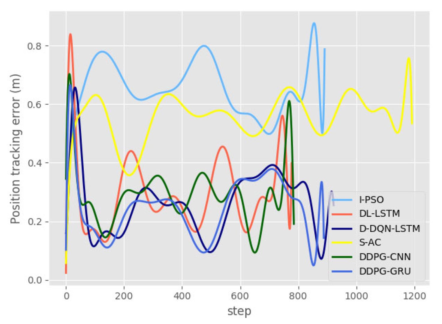
In Figure 12, when the AUV encounters an obstacle, it will adjust its heading to avoid the obstacle, and when there is no obstacle, it will maintain a constant heading. By inputting the desired heading angle and track points into the AUV model, we obtain the error curve of the control algorithm. It can be seen from Figure 13 that under the action of the control algorithm, the error of the control signal heading angle becomes smaller. Upon reaching the target point, the root mean square (RMS) error of the I-PSO algorithm is the smallest, while that of the S-AC algorithm is the largest. The position tracking error curve in Figure 14 is obtained by fitting. It can be seen from the figure that the error is less than 1 m during the whole track point tracking process. At the endpoint, the error for D-DQN-LSTM, I-PSO and DDPG-GRU is approximately 0.5 m, while that for S-AC and DDPC-CNN exceeds 0.7 m.

Figure 15 shows the torque change curve of the AUV thruster. Figure 16 is a sampling diagram of Figure 15, which is obtained every 10 times. It can be seen from Figure 15 that the maximum output torque of the S-AC and DDPG-CNN thrusters reaches 80 N·m, and the turning angle planned by the algorithm can be completed. At the same time, there is a part of the torque of the propeller to eliminate the influence of ocean currents. So, even if the steering angle is 0, the output torque at this time is not 0.

Figure 16 presents a segment of the complete data, specifically the range [3500, 3640], which corresponds to [350, 364] in Figure 15. The figure also shows that the instantaneous output torque of the S-AC and DDPG algorithms is greater than that of the other four algorithms. The I-PSO and D-DQN-LSTM algorithms exhibit the smallest torque changes.

4.2.4. Maze Environment

Figure 17 is a complex maze, with a start point [70, 100], an end point [584, 448] and static square and circular obstacles. The parameters of the I-PSO algorithm are the population size $M=100,\mathrm{N}=280$, $c_1{r}_1=0.7,c_2{r}_2=0.6$. The speed of the ocean current is $0.2 \mathrm{m}/\mathrm{s}$ and the direction is $\frac{\pi }{6}$. The paths planned by the six algorithms are shown in Figure 17. It is intuitively observed that the trajectory of the DDPG-CNN algorithm is the longest.

According to

Table 4. Comparison of trajectory length and time of various algorithms in a maze environment.

Title 1	Time (min)	Path Length (m)
I-PSO	43.68	4518
DL-LSTM	40.80	4720
D-DQN-LSTM	40.41	4716
S-AC	40.13	4680
DDPG-CNN	39.78	4626
DDPG-GRU	38.69	4566

, the I-PSO algorithm has the shortest path, while the DL-LSTM has the longest. The difference in path length between DDPG-GRU and I-PSO is not significant. In terms of time, I-PSO takes the longest time and DDPG-GRU is the shortest.

Figure 18 shows the change curve of the heading angle of the six algorithms. The heading angle change trends of the DDPG-GRU and I-PSO algorithms are similar, as are those of the S-AC and DL-LSTM. In Figure 19, the RMS error of the I-PSO is the smallest, while DDPG-CNN’s is the largest, with D-DQN-LSTM and DDPG-GRU showing almost identical values. After reaching the target point in Figure 20, the position tracking error is smallest for DDPG-GRU at 0.4 m and largest for DL-LSTM at 0.8 m.

Figure 21 shows the output torque curve of the thruster during AUV navigation. The torque of the S-AC, DDPG-CNN and DDPG-GRU algorithms reaches the range of [−80, 80], while the output torque of I-PSO and DL-LSTM, mostly within [−60, 60], and rarely reaches [−80, 80]. Figure 22 presents a segment of the complete data, specifically [3500, 3640], which corresponds to [350, 364] in Figure 21. It can be seen from the figure that the torque fluctuation of the D-DQN-LSTM algorithm is the smallest at this stage.

4.2.5. Dynamic Environment

Figure 23 tests the planning ability of various algorithms in an environment containing dynamic obstacles. As shown in the figure, the AUV start point is [50, 400] and end point is [1195, 472], in addition to adding rectangular obstacles. The parameters of the I-PSO algorithm are the population size $M=160, \mathrm{N}=390$, $c_1{r}_1=1.4, c_2{r}_2=1.8$. The speed of the ocean current is $0.3 \mathrm{m}/\mathrm{s}$ and the direction is $-\frac{\pi }{6}$. The speeds of moving obstacles 1 and 2 are both 0.5 m/s, the heading angle of the moving obstacle 1 is 270° and the heading angle of the moving obstacle 2 is 0°. Since the trajectory of the dynamic obstacle 1, 2 in the red rectangular box covers the rest of the algorithm trajectory, it is not displayed completely.

In

Table 5. Comparison of trajectory length and time of various algorithms in a dynamic environment.

Title 1	Time (min)	Path Length (m)
I-PSO	43.68	4518
DL-LSTM	40.80	4720
D-DQN-LSTM	40.41	4716
S-AC	40.13	4680
DDPG-CNN	39.78	4626
DDPG-GRU	38.69	4566

, the DL-LSTM algorithm shows the shortest time and path, while the S-AC algorithm has the longest. DDPG-CNN and DL-LSTM are very close in time and trajectory length. The distance between DDPG-GRU and I-PSO is only 6 m, but the time difference is 150 s. This is due to the single-step planning time of I-PSO being about 10-times longer than that of DDPG.

Figure 24 shows that the heading curves of I-PSO and DDPG-GRU are highly consistent. After encountering an obstacle for the first time, DL-LSTM made the collision avoidance strategy opposite to the I-PSO algorithm, while DDPG-CNN, DDPG-GRU and the I-PSO algorithm have the same strategy. When the AUV detects an obstacle for the first time in Figure 24, the planned heading angle changes sharply. In Figure 25, D-DQN-LSTM has the smallest RMS, DL-LSTM has the largest and I-PSO and DDPG-GRU are almost the same. After the position tracking error curve in Figure 26 reaches the target point, the smallest is DDPG-GRU, and the largest is I-PSO. The position tracking error of all algorithms does not exceed 1 m in the whole process.

In order to achieve this goal under the influence of ocean currents, the propeller needs to output more torque. In Figure 27, at around 100 steps, the output torque of each algorithm exceeds 40 N·m. After encountering dynamic obstacles 1 and 2, several algorithms adopted completely different collision avoidance strategies. Figure 28 presents a segment of the complete data, specifically [3500, 3640], corresponding to [350, 364] in Figure 27. It can be seen from Figure 28 that the propeller output torque of the D-DQN-LSTM and DDPG-GRU algorithms has smaller fluctuations than other algorithms.

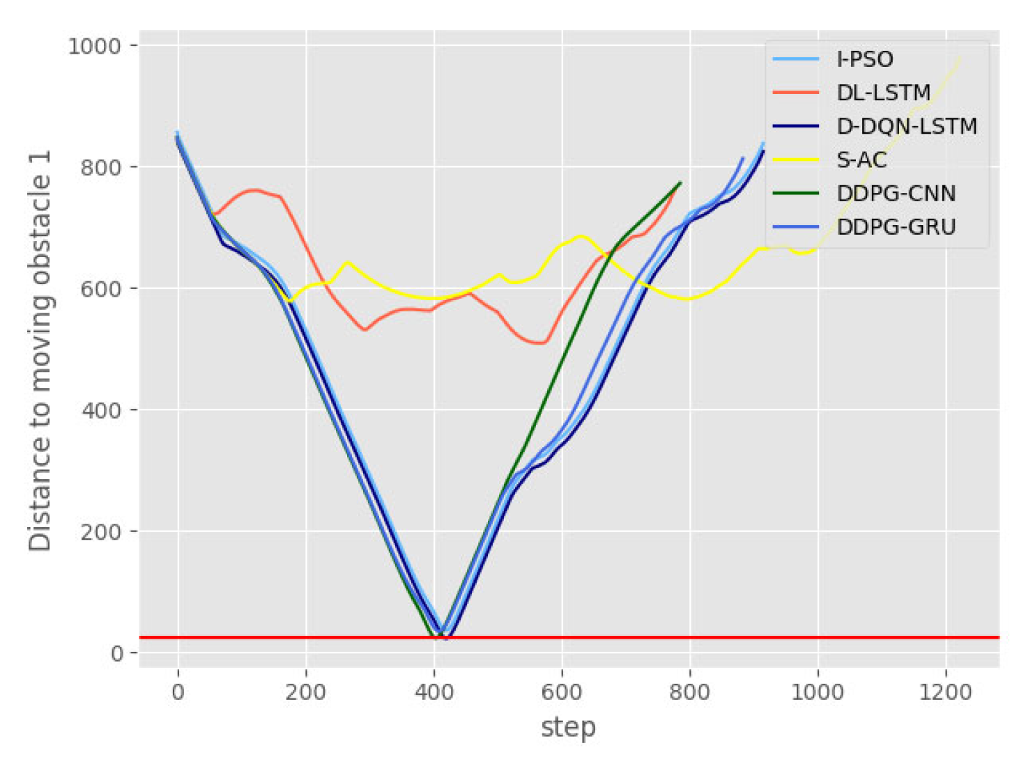
Figure 29 and Figure 30 show the distance curves between the AUV and dynamic obstacles. The horizontal red line in the figures represents a distance of 25 m, indicating the collision threshold between the AUV and a dynamic obstacle. Figure 29 shows that at about 400 steps, the D-DQN-LSTM and DDPG-CNN algorithms both collided with the dynamic obstacle 1. I-PSO and DDPG-GRU did not collide with obstacle 1, but their planned trajectories were closer than the safe distance to obstacle 1. None of the algorithms in Figure 30 collided with obstacle 2. The distances between D-DQN-LSTM, S-AC and DDPG-GRU and the obstacle were less than the safe distance.

4.3. Result Analysis

In static and dynamic environments, the heading angle adjustment of I-PSO and DDPG-GRU is the smallest, followed by the DL-LSTM and D-DQN-LSTM algorithms. The control signal RMS error curves in Figure 13, Figure 19 and Figure 25 show that the error decreases with time. Figure 14, Figure 20 and Figure 26 show that the position tracking error changes over time. The maximum value is 1.24 m in the maze environment, and it does not exceed 1 m in both static and dynamic environments. Figure 15, Figure 21 and Figure 27 show that the output torque of the DDPG-GRU thruster is lower than that of S-AC. The lower output power not only saves energy consumption but also prolongs the service life of the propeller. Figure 29 and Figure 30 show that the I-PSO algorithm and DL-LSTM also avoid dynamic obstacles. Compared with the other three DQN algorithms, the DDPG-GRU algorithm can safely avoid dynamic obstacles. The simulation experiment of robustness and stability shows that the algorithm based on DDPG is better than other algorithms. The experimental results in the latter three environments show that the comprehensive ability of the DDPG algorithm for collision avoidance planning is far superior to several other DQN algorithms, DL algorithms and even I-PSO (this algorithm is based on all known environmental information).

The I-PSO algorithm needs to use different parameters for different environments to achieve excellent planning results, which requires expert experience. When the environment becomes complicated, the generation time of the single-step strategy of the I-PSO algorithm has a greater impact than other algorithms, because it requires constant iteration to find the optimal path. Compared with the I-PSO algorithm, the deep learning obstacle avoidance planning algorithm can be completed in a shorter time, but it still needs to use a large number of samples for offline learning. Such training samples can be generated by various intelligent algorithms, but the quality of the training samples, network structure and parameters will all affect the network model. Because the recurrent neural network has strong associative memory capabilities, it is very suitable for processing sequence data. The DQN algorithm, a reactive learning method, continuously learns based on rewards and is suitable for both online and offline learning. In addition, the learning samples are self-generated, which significantly reduces development and deployment time compared to DL-LSTM with additional algorithms.

5. Conclusions

Traditional path planning algorithms rely on an accurate environmental map, where readapting the generated path can be highly demanding in terms of computational cost. This paper proposes a DRL obstacle avoidance algorithm for the AUV in environments with unknown dynamics. This paper primarily focuses on a method to realize the AUV’s reactive collision avoidance behavior by determining the mapping between perceptual information and action through learning the reward function. Although the algorithm proposed in this paper achieved good results, there are still many problems that have not been solved. The reward function is difficult to switch adaptively between different environments and obstacles. In future research, we plan to adopt the inverse reinforcement learning (IRL) method [52] so that the AUV can learn the reward function by itself, and no manual or expert setting is required. Our method still has some limitations, most notably that, like most model-free approaches, DDPG requires a large training set to find a solution. Since the sonar data observed by AUV are a series of sequence data, we are also considering introducing the Transformer model [53] with an attention mechanism into the path planning field in the future.