
Integrating k-means Clustering and LSTM for Enhanced Ship Heading Prediction in Oblique Stern Wave
College of Ocean Science and Engineering, Shanghai Maritime University, Shanghai 201306, China
*
Author to whom correspondence should be addressed.
J. Mar. Sci. Eng. 2023, 11(11), 2185; https://doi.org/10.3390/jmse11112185
Submission received: 21 October 2023
/
Revised: 6 November 2023
/
Accepted: 10 November 2023
/
Published: 17 November 2023
(This article belongs to the Section Ocean Engineering)
Abstract
:The stability of navigation in waves is crucial for ships, and the effect of the waves on navigation stability is complicated. Hence, the LSTM neural network technique is applied to predict the course changing of a ship in different wave conditions, where K-means clustering analysis is used for the category of the ship’s navigation data to improve the quality of the database. In this paper, the effect of the initial database obtained by the K-means clustering analysis on prediction accuracy is studied first. Then, different input features are used to establish the database to train the neural network, and the influence of the database by different input features on the accuracy of the navigation prediction is discussed and analyzed. Finally, multi-task learning is used to make the neural network better predict the navigation in various wave conditions. Using the improved neural network model, the course of an autopilot ship in waves is predicted, and the results show that the current database and the neural network model are accurate enough for the course prediction of the autopilot ship in waves.
1. Introduction
The interaction and movement between ships and waves are of utmost importance for ship handling and safety at sea. Understanding how waves influence a ship’s behavior, stability, and navigational challenges is vital to ensuring the safety of vessels, crew, cargo, and the environment. This helps optimize ship handling, cargo stability, emergency response, and vessel design while minimizing environmental impact. In the maritime industry, accurate predictions and models of ship–wave interactions are essential for enhancing safety, efficiency, and overall operational excellence.
With the increasing demand for ship motion prediction, researchers are improving traditional prediction methods. Triantafyllou and Bodson (1983) [1] applied Kalman filtering techniques to estimate the complex ship’s motions. However, a significant limitation arose from nonminimum phase characteristics due to the spatial integration of water wave forces, resulting in an irrational and nonminimum phase transfer matrix function. Sutulo S (2002) [2] studied ship maneuvering simulations, focusing on two essential methods: dynamic and kinematic prediction models, emphasizing improved kinematic prediction techniques. Rigatos (2013) [3] explored dynamic ship positioning using sensor fusion techniques based on Kalman and Particle Filtering algorithms, while Perera (2017) [4] used an extended Kalman filter and vector-based algorithms for short-term ship maneuver prediction. Fossen (2018) [5] introduced an exogenous Kalman filtering (XKF)-based ship motion prediction method, leveraging real-time Automatic Identification System (AIS) data for visualization and motion prediction. Jiang H et al. (2020) [6] studied the scale effects of autoregressive (AR) models in real-time ship motion prediction, enhancing prediction accuracy and providing valuable guidance for real-time prediction. Luo W et al. (2020) [7] proposed a vector analysis-based ship motion and trajectory prediction method that analyzes ship movement vectors and velocities, constructing a concise and efficient prediction model capable of accurately predicting ship motion trajectories in complex marine environments. These methods primarily rely on prior knowledge and existing data for ship trajectory prediction. However, due to the complex and variable nature of the marine environment, the prediction performance of these methods has certain limitations.
Researchers have also continued to explore the detection and prediction of ship motion states, gradually shifting from traditional mathematical model-based prediction methods to machine learning and deep learning-based methods, which have increased the reliability and performance of their predictions. Shen Y (2005) [8] explored the application of diagonal recurrent neural networks (DRNN) for predicting complex movements in large-scale ships affected by nonlinear and random factors, demonstrating improved prediction accuracy and stability. Khan et al. (2007) [9] explored using artificial neural networks, trained with singular value decomposition and conjugate gradient algorithms, to predict ship motion accurately. Ge et al. (2017) [10] presented a BP neural network-based motion attitude prediction method to enhance prediction accuracy and speed for ship motion compensation systems, addressing the challenge of obtaining timely specific motion features. Chen X et al. (2020) [11] introduced a convolutional neural network (CNN) based method for ship movement classification, providing an effective tool for ship trajectory prediction and monitoring. Zhang T et al. (2021) [12] introduced a multiscale attention-based LSTM model for ship motion prediction, utilizing attention mechanisms to capture information at different time scales, resulting in superior predictive performance. Bassam et al. (2022) [13] explored machine learning-based ship speed prediction, and various machine learning methods were compared, such as random forests and support vector machines, and demonstrated the effectiveness of these methods in predicting a ship’s speed to support efficient shipping operations. As technology advances, these methods will be further refined and optimized to provide better support for safe ship navigation. Kong Z et al. (2022) [14] developed a context-enhanced trajectory-based ship target recognition method that leverages the contextual information of ship trajectory data to improve target recognition accuracy. Abebe et al. (2022) [15] proposed a hybrid ARIMA–LSTM model for ship trajectory planning, offering more accurate ship trajectory prediction and collision avoidance planning.
In recent years, more and more scholars have used machine learning and deep learning to predict ship motion, among which the LSTM neural network has received more attention because of its excellent ability to process time series data. However, the features of the wave conditions are usually not taken into account when establishing the database and training the neural network. It has been noticed that the course stability and motion of the ship navigation are significantly influenced by wave conditions [16]. Hence, the wave features and ship motion characteristics are combined in this paper to establish the database for the neural network training, which aims to improve the accuracy of the course prediction for the ship sailing in various wave conditions.
In this paper, based on the navigation data of a ship sailing in different wave conditions at various initial forward speeds that have been published in our previous work [17], the navigation data of the autopilot ship in different sea conditions are classified by the k-means clustering method firstly, and the prediction accuracy of the neural network model trained by the classified data was analyzed. Secondly, the wave and ship motion are used as the input features of the database for training, and the effect of the different input features on prediction accuracy is studied. Finally, navigation data of an autopilot ship in a series of wave conditions are learned by the neural network at the same time, and the course of the ship in a new wave condition is predicted by the improved policy for neural network training. In this paper, the LSTM neural network model is used to predict the heading change. Through the comparison and discussion of various prediction policy, the influence of input feature combination, the number of datasets, and the classification of datasets on the accuracy of the model is discussed. Compared with the traditional LSTM neural network model, the optimized policy in this paper can better ensure the prediction accuracy and reliability of the results. The LSTM-based course prediction process of an autopilot ship in waves is shown in Figure 1.
2. Principles and Methods
2.1. k-means Clustering
The K-means clustering algorithm is an unsupervised learning method to obtain or reveal data’s intrinsic attributes and rules. The central principle of K-means is to partition the data into clusters based on similarity, where data points within the same cluster are more like each other than data points in other clusters [18]. The algorithm aims to minimize the sum of squared distances between data points and their respective cluster centers.
K-means starts by randomly selecting initial cluster centers (centroid points) within the feature space. These centers are represented as vectors in the same space as your data. The algorithm uses a distance metric to measure the similarity or dissimilarity between data points. The most common distance metric in K-means is the Euclidean distance. It calculates the straight-line distance between two data points in the feature space. The Euclidean distance formula used in this paper is defined as:
where and are two sequence points, represents the dimension.
For each data point, K-means assigns it to the cluster whose centroid is closest, based on the Euclidean distance. After assigning data points to clusters, the cluster centers are updated as the mean (average) of all data points within the cluster. The formula for updating the can be represented as:
where represents the number of data points assigned to the cluster .
The above assignment and updating steps are repeated iteratively. Data points are reassigned to the nearest cluster, and cluster centers are recalculated until convergence. The calculation formula for the iteration of the clustering center is:
where K is the optimal number of clusters.
2.2. RNN and the LSTM Model
Neural networks (NN) are computational models inspired by biological neural systems aimed at intelligent information processing [19]. NN training aims to find the optimal weight matrix that minimizes a given loss function. This training process relies on gradient descent optimization [20]. Backpropagation calculates the weight gradient of the loss function and updates the weights in the direction of the gradient to progressively reduce the loss function’s value. More precisely, for loss function , the update formulas for weights and biases are as follows:
where is the learning rate, is the layer, and and are the indices of the neurons.
Long Short-Term Memory (LSTM) is a specialized recurrent neural network (RNN) for sequential data processing. While RNNs can capture temporal dependencies, they face challenges with vanishing and exploding gradients when dealing with long sequences, limiting their learning abilities. LSTM, introduced by Hochreiter and Schmidhuber (1997), [21] addresses this issue. It overcomes the problems faced by traditional RNNs by incorporating gating mechanisms and memory cells [22]. LSTM’s structure includes forget gates, input gates, output gates, and memory cells, which collectively learn and maintain long-term and short-term dependencies. The forget gate decides which historical information to keep, the input gate controls the impact of the current input on the memory cell, and the output gate determines the hidden state to pass to the next timestep or output layer. These gating structures allow LSTM to effectively process long sequences by learning and retaining important information across different time scales. Refer to Figure 2 for the structure diagram.
In particular, the critical equations in LSTM are as follows:
where (, , ) is the activation values of the input, forget, and output gates, respectively. where is the candidate memory cell, while and correspond to the memory cell and hidden state of the LSTM unit, respectively. and denote the weight matrices and bias vectors, signifies element-wise multiplication, and is the sigmoid activation function.
2.3. Data Normalization
Data processing is essential to ensure the reliability and robustness of the prediction model. The data normalization is used in this paper to address potential differences within the range of input features, by which the data points are expanded linearly to the common range. To this end, we utilize the MinMaxScaler from the scikit-learn library for normalization (Kramer O et al., 2016 [23]). The scaler achieves this transformation by applying the following formula to each feature
where represents the normalized value, is the original value, and denote the minimum and maximum values of the feature, respectively. This transformation maps each feature to a specified range, typically [0, 1], while preserving the original distribution and relative distances between data points. The dataset in this paper includes various features such as ship motion, rudder angle, speed, drift angle, force, and torque, and we can effectively decrease potential biases caused by different measurement scales by applying the MinMaxScaler to the database.
2.4. LSTM Input and Output Data Mapping
The LSTM neural network can process multi-feature inputs. During the training process, it is essential to create a mapping relationship between input duration data and the corresponding output duration data , where denotes the various input feature types, and denotes the time series. This mapping is achieved with a sliding window technique, by which the neural network could process the time series data effectively.
To achieve this, we employ a sliding window technique to segment the complete time series, = {}, with data points, into a collection of input–output pairs. Each pair consists of an input sequence of length k, represented as {}, and a corresponding output sequence of length , represented as {}, where denotes the delay time of prediction. The output sequence can also be expressed as {}. This process yields time series, facilitating exploring the mapping relationship between input and output sequences. In this article, window sliding is divided into the training part and the prediction part. During data training, the input sample of length is used to output the output sample of length , as shown in 0(a). The input window of each prediction is sequential data, and then the next data are predicted. Meanwhile, the last forecasted result is taken as a part of the next input, which is presented as appended data. This means that each prediction step uses previous predictions, and the output of each prediction is continuous, as shown in Figure 3b.
3. Data from the Autopilot of Ship in Waves
3.1. The Autopilot of Ship in Waves
The data of an autopilot trimaran in quartering seas are used in this paper as the database for training and prediction. The data of the autopilot trimaran sailing in quartering seas of various features at different speeds are obtained by a hybrid method developed by the open-source CFD tool OpenFOAM and called qaleFoam. With the hybrid method, the nonlinear effects could be considered during the simulation of course keeping, course instability, and broaching-to, such as side-hull emergence, bow diving, and transient draft variation. The quartering seas are simulated because it will lead to the instability of the course and even broaching-to. For the reason that a part of the computed results has been published in our previous work, it is only introduced briefly here for the completeness of this paper.
In the internal domain of the hybrid method, the ship motion and the ship–wave interaction are simulated by the incompressible URANS, which can be expressed as
where is density, is time, is the gravitational acceleration, is the velocity field, is the moving velocity of the grid, is the dynamic pressure field, is the effective dynamic viscosity, is the surface tension term, and is the source term. The VOF and compression techniques are applied to simulate the Euler two-phase flow. An artificial compression technique (Rusche, 2002; Weller, 2002 [24,25]) is used in OpenFOAM to ensure that the value is consecutive and that the non-zero value only appears at the interface between air and water.
During the ship’s autopilot in waves, the internal domain moves with the ship within the external domain. The fluid is assumed to be ideal in the external domain, and the velocity potential satisfies the Laplace equation. One side of the external domain features a wavemaker, while the other employs a self-adaptive wavemaker for wave absorption. The free surface ensures the satisfaction of both kinematic and dynamic boundaries. The interfaces and transition zone establish the connection between the two domains. Because the hybrid method has been applied for different issues on FSI, more details about the QALE-FEM and the hybrid method could refer to the reference (Ma et al., 2009; Yan et al., 2010; Hu et al., 2020; Gong et al., 2021 [26,27,28,29]).
A global coordinate system (, , ) is employed to solve the flow field. In ship motion analysis, a local coordinate system (, , ) is utilized, with its center coinciding with the trimaran’s center of gravity. This approach helps avoid the need for force and moment corrections. The methodology for solving the trimaran’s six degrees of freedom (6DOF) motion is based on the reference work by Xing et al. (2008) [30].
Trimaran’s motion is divided into linear and rotational components in the local coordinate system. The linear motion is described by the velocities (, , ) and their corresponding acceleration rates. On the other hand, the rotational motion is represented by the angular velocities (, , ) and their corresponding angular acceleration rates. The overall motion and rotation of the trimaran are governed by the 6DOF maneuvering equations.
where is the mass of the trimaran, (, , ) is the inertia moment, (, , ) and (, , ) are the total force and moment of the hull surface, which are obtained by the solution of the internal viscous-flow domain in every time step, and the force and moment by the effect of velocity, acceleration velocity, pressure, and viscosity are taken into account. (, , ) and (, , ) is the force and moment of the water jet impetus. The roll, pitch, and yaw angle are expressed by the Euler angle (, , ) (Gong et al., 2022 [17]). After Equation (8) is solved, the changing rate of the Euler angle could be obtained by
For simulating the autopilot system of the trimaran, a semi-empirical model based on Renilson et al. (1998) [31] and Jong et al. (2013) [32] is employed to capture the water-jet thrust and steering moment characteristics. The autopilot utilizes a proportional-derivative (PD) control scheme. The desired target heading is set to 0°, while the yaw angle error in each time step and its corresponding angular velocity represent the deviation and its rate of change, respectively. In order to facilitate the distinction, the motions of heave, roll, and pitch are expressed by , , , the heading is expressed by , which is the same to .
3.2. Wave and Ship Motion Data
Wave conditions directly impact ship navigation (Ivan et al. 2012 [33]), and the values of / and are vital factors for the course stability of ships in waves (Gong et al., 2022; Jong et al., 2013 [17,32]), where is the initial ship speed, is the wave propagation speed, and are the wavelength and wave height. Therefore, in this paper, all navigation data are classified based on special criteria, which include the values of / and . The navigation data of the ship sailing in different wave conditions at various initial forward speeds are used to establish the database and train the neural network, which has been published in our previous work (Gong et al., 2022 [17]).
In this study, represents course deviation from the original course. In addition to the existing initial features of the ship sailing, the influence of the following features on the course stability of the ship will also be discussed. According to the objective of this study and the navigation data of the ship, the classification of input features used in this paper is shown in Table 1, where (, , ) the hydrodynamic force acting on the hull surface, (, , ) is the corresponding moment, is the nozzle deflection angle, and are the surge and sway of the ship.
4. Model Construction and Evaluation
4.1. Model Structure and Initial Features
Table 2 shows the neural network’s essential structure and the initial setting of related parameters. This study utilized a model architecture based on LSTM recurrent neural networks for time series prediction. The model consisted of two LSTM layers with dropout layers for regularization. A dense layer with ReLU activation was employed for generating predictions. The data were normalized using the MinMaxScaler technique to ensure optimal model performance. The integration of LSTM layers, dropout layers, and ReLU activation enhanced the model’s ability to capture complex temporal patterns. Data normalization facilitated training convergence and reliable predictions. The accurate time series predictions could be achieved by fine-tuning the model and adapting it to the dataset’s characteristics.
4.2. Performance Evaluation and Optimization
In this research, the performance evaluation and optimization of the code were conducted to ensure the effectiveness of the time series prediction model. The performance of the model was assessed using various evaluation metrics, such as mean squared error (MSE), root mean squared error (RMSE), and mean absolute error (MAE). These metrics were employed to quantify the accuracy and precision of the model’s predictions. It is calculated as follows:
In order to optimize the model, several strategies were implemented. The model architecture was fine-tuned by adjusting the number of LSTM layers, neurons per layer, and dropout rate. Data preprocessing techniques were applied to improve the data quality, including feature selection, normalization, and handling missing values. Performance evaluation was conducted on training and validation sets to detect overfitting and improve generalization. The model’s performance was optimized through these processes, and more accurate and robust time series predictions could be achieved.
5. Prediction Based on the LSTM
5.1. Selection Process for Input Length
This section aims to find the optimal time series input length k to predict the data at timestep k + 1. Five input lengths (k = 250, 500, 750, 1000, and 1500) have been chosen to compare prediction accuracy. Because of the accumulation of errors during the prediction process, the main error between the predicted data and the original data mainly appears after t = 30 s. Hence, the predicted data and the original data between 30 s and 40 s are used for comparison in this paper.
The prediction results by different input data lengths are shown in Figure 4. predicted by LSTM of different input lengths, and the performance evaluation has been listed in Table 3. It can be seen that the accuracy of the neural network has increased with the growth of input length, especially between 250 and 1000. However, the accuracy of the neural network model starts to decrease when the length exceeds 1000, and it probably means the existence of an optimal input length corresponding to the best prediction accuracy. The reason is that the increase in input lengths of data could lead to better training results, but it will also produce more error accumulation with the increase in the input length k used for training. Hence, k = 1000 is used as the input length for training.
5.2. Prediction Based on the Data after k-means Clustering
In this paper, a K-means clustering model based on the values is used to cluster the navigation data of the autopilot ship in different sea conditions. By continuously optimizing the parameters of the clustering model, the classification performance of the clustering model meets the expectation. At this time, the K-means model is configured with 3 clusters, 123 random seeds, and the initial center point selection is iterated 20 times. After completing the classification, the model assigns a clustering label to each file, effectively dividing them into groups based on their similarity of the tendency.
The classification results are illustrated in Figure 5. After clustering, 34 datasets were divided into three categories, named Group1, Group2, and Group3. Three groups of random data are taken from Group1 (Data1, Data2, Data3), Group2 (Data4, Data5, Data6), and Group3 (Data7, Data8, Data9). Comparing Figure 6a, Figure 6b and Figure 6c, it can be seen that each combination will have significant differences in amplitude, period, and overall trend convergence. Three groups of navigation data in Group1 were selected for training and prediction, and the values of their initial features are shown in Table 4.
In this section, Data1 and Data2 from Group1 were selected as the training sets. The model was trained separately on each dataset to capture their unique characteristics. Then, Data3 is predicted, respectively, and the comparison between the actual trend and the predicted trend is shown in Figure 7a,b. To further compare the model’s performance, Data4 in Group2 and Data7 in Group3 are selected as training sets, respectively, and the comparison between the actual trend and the predicted trend is shown in Figure 7c,d. The comparative analysis of evaluation metrics is presented in Table 5.
It can be observed from Figure 7 that the prediction performance of Figure 7a,b is better than that of Figure 7c,d. Further combining the differences of evaluation metrics in Table 5, the Data2 dataset achieves better performance when training the model. This model trained under Data2 has lower MSE, RMSE, and MAE. This means that the average difference between the predictions on Data2 and the original data is small and has better accuracy. In contrast, the Data7 dataset produced the worst results in model training. The model has a larger MSE, which indicates that the prediction error of the model on Data7 is large, and there is a significant difference between the prediction and the original data. The performance of the models trained under Data1 and Data4 datasets is between Data2 and Data7.
Some reasons can be found in Figure 7d for the extremely poor prediction performance on Data7. Based on the data trends, the gap between Group3 and Group1 is far more significant than the gap between Group2 and Group1. Considering the grouping situation of cluster analysis and the trend comparison of each group in Figure 7, the training performance of Data4 is better than that of Data7. Hence, it can be preliminarily concluded that cluster analysis can improve the accuracy of the LSTM neural network model to a certain extent. In order to further verify this point of view, this paper adds two sets of prediction results. Training the model on Data5, and then making predictions on Data6. The same is performed for Data8 and Data9. Figure 8a,b shows the two prediction results.
From Figure 8a, it can be found that prediction accuracy meets expectations. The further analysis combined with Table 6 shows that the prediction of Data6 achieves an ideal prediction performance, while for the prediction of Data9, although the MSE is not ideal, the values of RMSE and MAE have reached a relatively small level. To sum up, after training between datasets with large trend gaps, the prediction results are often unsatisfactory, but within a specific range, cluster analysis can optimize this result and improve the accuracy of the LSTM neural network.
5.3. The Effect of Input Features
Applying each feature group to the model aims to identify the features that significantly influence the prediction performance. This process involved comparing the prediction results obtained from each feature group and analyzing their respective impact on the accuracy and reliability of the prediction performance. The neural network model learns various features of navigation data under one sailing condition, saves the trained model, and then predicts the course change under other sailing conditions. The MSE, RMSE, and MAE are calculated for each of the six datasets to evaluate the model’s performance.
The prediction results for full features are shown in Figure 9. The prediction results for full features are shown in Figure 9. Table 7 shows the initial conditions for the selected training and test sets. The prediction results of full features can be used as one of the criteria to judge the prediction performance of each set of feature combinations.
In Figure 10, it can be seen that after removing the features of trajectory, speed, and torque, the gap between the prediction and the original data is significant. Combining the changes in MSE, RMSE, and MAE values under various conditions is necessary for further analysis. In Table 8, we can observe that a decrease in MAE, MSE, and RMSE is evident when the torque feature and the force-feature are removed from the database, which means prediction accuracy is improved. Remarkably, we found that removing the influence of the force feature had a significant positive impact on the prediction performance. It also means that the force feature could negatively influence the prediction performance. However, upon removing the motion feature, we observed a slight deterioration in the prediction performance. Both MSE and RMSE increased, accompanied by a rise in MAE, indicating the importance of this feature in achieving accurate predictions. Similarly, excluding the speed feature resulted in a substantial decline in the prediction performance will lead to higher values of MSE, RMSE, and MAE, which means the necessity of this feature on the accuracy of the predictions. It could also be found that removing the trajectory feature had a noticeable negative impact on the prediction performance. The increase in MSE, RMSE, and MAE indicated the significance of this feature in achieving accurate predictions. Conversely, removing the influence of the feature led to a slight improvement in the model’s predictive performance. The decrease in MSE, RMSE, and MAE implied a potential positive effect of removing this feature.
Our analysis revealed that removing the force features yielded the most substantial improvement in the model’s predictive performance. Conversely, the exclusion of the speed-features and trajectory-features resulted in a significant decrease in accuracy. Considering these findings, decreasing the influence of the force-features is recommended to achieve optimal prediction results. For each type of feature, there are multiple dimensions of data. The L2 norm of each type of feature can be taken to compress the latitude and reduce the effect of error accumulation.
5.4. Comparisons of Multi-Task Learning
In this section, multiple datasets are introduced simultaneously for training, focusing on the result of K-means clustering. The aim is to discover if there is an optimal number of datasets to achieve the best prediction performance. The model will be trained with one to six data groups, respectively, and the final prediction results will be compared. The six groups of data were named {TrainingD1, TrainingD2... TrainingD6}, their initial features are shown in Table 9. And the number of datasets for training was successively increased. Notably, this paper incorporates initial features as independent features in the training data. By including initial features, shown in Table 9, as a separate feature column, the model can directly capture the relationship between these features and the others, leading to improved understanding and prediction of model performance. We can assess their influence by comparing the final prediction results obtained from different numbers of training sets. The prediction results for different numbers of training sets are visually represented in Figure 11, while specific performance metrics such as mean squared error (MSE), root mean squared error (RMSE), and mean absolute error (MAE) are summarized in Table 10.
In the analysis of the results, it was observed that when training was conducted using a single dataset, as depicted in Figure 11a, the predicted outcomes exhibited a substantial margin of error. Nevertheless, Figure 11b showcases a marked improvement, wherein training with two distinct datasets resulted in predicted trends that approached the reference values (MSE, RMSE, and MAE), thereby achieving comparable predictive efficacy as the earlier employed clustering analysis.
As the experiment progressed from Figure 11c to Figure 11f, each iteration entailing an incremental increase in the number of training datasets, a discernible enhancement in the accuracy of predictions was witnessed. The quantification of prediction errors using metrics such as MSE, RMSE, and MAE substantiated this observation, with diminishing values signifying prediction closer to the original data.
More specifically, when training encompassed two datasets, the accuracy of the neural network model has increased significantly. Including three, four, five, and six datasets for training purposes led to further reductions in prediction errors, thus exemplifying a noteworthy augmentation in precision. However, when the number of datasets has increased to four, the performance improvement of the model begins to flatten out, and the benefits brought by increasing the number of datasets gradually decrease.
In summary, multi-task learning can significantly improve the prediction performance of the model, but multi-task also brings more computational effort. It is necessary to maintain a balance between increasing the dataset to improve prediction accuracy and increasing the amount of computation. Therefore, in practical applications, choosing the optimal number of datasets can enable the model to maximize its performance.
5.5. Optimization Method Prediction
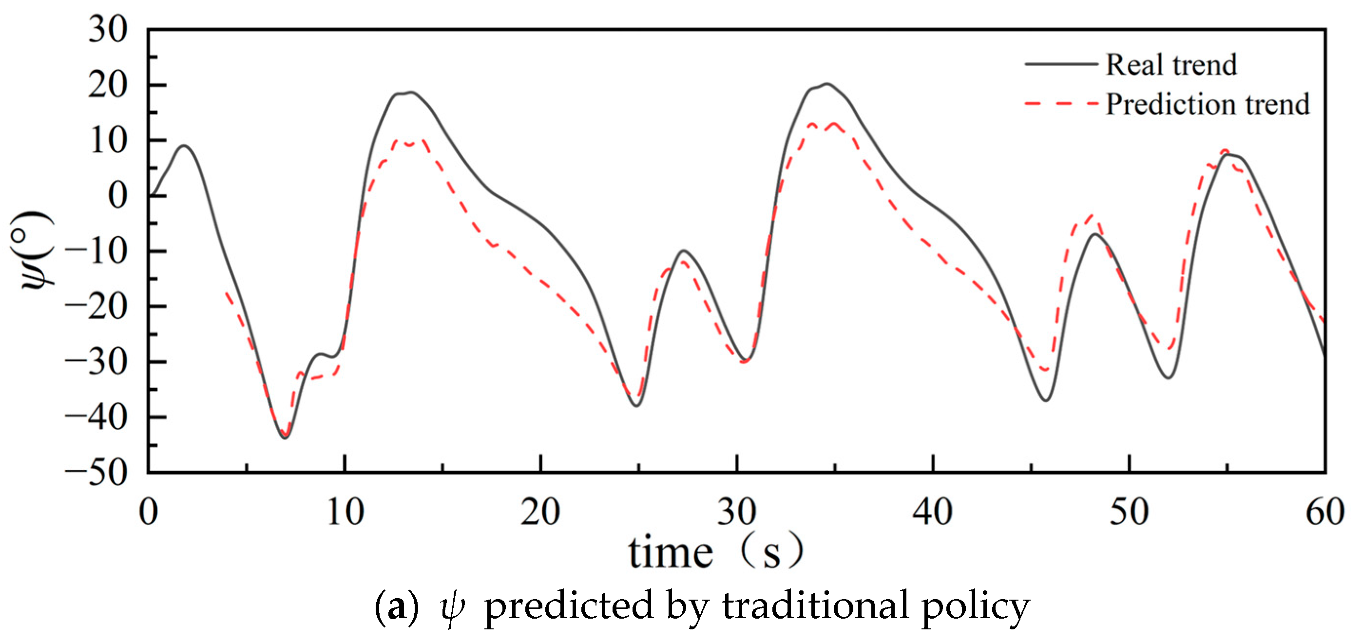
After conducting a comprehensive analysis of various combinations of input features, it has been observed that the impact of force features is negative. For the force feature, there are three dimensions of data. The L2 norm can be taken to compress the latitude and reduce the effect of error accumulation. Furthermore, by adopting a multi-task learning methodology, multiple datasets are analyzed in accordance with established patterns, with particular attention given to the initial wave and ship features. Six datasets from Group2 in Section 5.2 are selected for demonstration. Five groups are employed for training purposes to ensure robustness, where one group serves as the test set, as indicated in Table 11, which includes the compressed force-features data, thereby minimizing error accumulation. The predicted results are presented in Figure 12.
The comparison in Table 12 reveals that the predicted performance has smaller MSE, RMSE, and MAE values than the previous predictions. Figure 12 illustrates that the overall trend aligns closely with the actual data, demonstrating a high fitting level until around 15 s, with some deviation occurring afterward. Several speculations can be made to explain this observation. Firstly, additional unknown data scenarios might not be adequately learned during the training process, leading to decreased prediction accuracy. Secondly, noise or outliers within the dataset can adversely impact the prediction results. Furthermore, the complexity and feature settings of the model itself may contribute to the gradual increase in deviation during later predictions. Nonetheless, through continuous optimization and meticulous selection, the current experiment achieved a relatively accurate level of trimaran sailing forecast within the initial 15 s.
6. Conclusions
This study aims to apply the LSTM neural network model to predict the course changing of a trimaran in different wave conditions. The K-means clustering analysis is used for the navigation data category to improve the database’s quality. The effect of the features used to build the database on prediction accuracy is discussed. By the study results, the following conclusion can probably be drawn.
- (1)
- In this paper, K-means clustering is applied to the classification of trimaran sailing data. It is found from the comparison that the model trained by the datasets with similar trends could be of relatively better prediction accuracy. Evaluation metrics like MSE, RMSE, and MAE compared predictions of different data subsets. Clustered datasets showed similarities, with better predictions within the same group.
- (2)
- Our analysis evaluated the impact of various feature combinations on predictive performance. Removing the force feature significantly improved accuracy, reducing MSE, RMSE, and MAE values. Excluding the features of speed and trajectory led to accuracy deterioration. Feature selection is crucial for precise predictions and advancing predictive modeling.
- (3)
- Using multi-task learning, the predictive ability is enhanced. Training multiple datasets with different initial conditions enhanced predictive capability. Including more datasets improved accuracy by capturing complex relationships. Better utilizing available data is crucial for constructing predictive models.
In short, this study combines wave features and navigation attitude data and optimizes the heading prediction based on LSTM time series prediction through classification discussion and cluster analysis. Future studies could explore wave features and initial conditions to improve the performance and stability of ships in marine environments.
Author Contributions
Conceptualization J.X. and J.G.; methodology, J.X.; validation, J.X. and J.G.; formal analysis, L.W. and Y.L.; investigation, J.G. and L.W.; data curation, J.X. and J.G.; writing—original draft preparation, J.X. and L.W.; writing—review and editing, J.G. and Y.L.; supervision, J.G. and Y.L.; funding acquisition, J.G. and Y.L. All authors have read and agreed to the published version of the manuscript.
Funding
This project was supported by the Science and Technology Commission of Shanghai Municipality, China (Grant number 22YF1415900), and the National Natural Science Foundation of China (Grant number 52101359).
Institutional Review Board Statement
Not applicable.
Informed Consent Statement
Not applicable.
Data Availability Statement
No new data were created or analyzed in this study. Data sharing is not applicable to this article.
Acknowledgments
The authors wish to thank the anonymous reviewers whose valuable and helpful comments greatly improved the manuscript.
Conflicts of Interest
The authors declare that they have no known competing financial interest or personal relationship that could have influenced the work reported in this paper. The funders had no role in the design of the study; in the collection, analyses, or interpretation of data; in the writing of the manuscript; or in the decision to publish the results.
References
- Triantafyllou, M.; Bodson, M.; Athans, M. Real time estimation of ship motions using Kalman filtering techniques. IEEE J. Ocean. Eng. 1983, 8, 9–20. [Google Scholar] [CrossRef]
- Sutulo, S.; Moreira, L.; Soares, C.G. Mathematical models for ship path prediction in manoeuvring simulation systems. Ocean. Eng. 2002, 29, 1–19. [Google Scholar] [CrossRef]
- Rigatos, G.G. Sensor fusion-based dynamic positioning of ships using Extended Kalman and Particle Filtering. Robotica 2013, 31, 389–403. [Google Scholar] [CrossRef]
- Perera, L.P. Navigation vector based ship maneuvering prediction. Ocean. Eng. 2017, 138, 151–160. [Google Scholar] [CrossRef]
- Fossen, S.; Fossen, T.I. Exogenous Kalman Filter (xkf) for Visualization and Motion Prediction of Ships Using Live Automatic Identification Systems (ais) Data. 2018. Available online: http://hdl.handle.net/11250/2584706 (accessed on 1 April 2018).
- Jiang, H.; Duan, S.; Huang, L.; Han, Y.; Yang, H.; Ma, Q. Scale effects in AR model real-time ship motion prediction. Ocean. Eng. 2020, 203, 107202. [Google Scholar] [CrossRef]
- Luo, W.; Zhang, G. Ship motion trajectory and prediction based on vector analysis. J. Coast. Res. 2020, 95, 1183–1188. [Google Scholar] [CrossRef]
- Shen, Y. On the Neural Network Theory and Its Application in Ship Motion Prediction. Ph.D. Thesis, Harbin Engineering University, Harbin, China, 2005; pp. 5–83. [Google Scholar]
- Khan, A.; Marion, K.; Bil, C. The prediction of ship motions and attitudes using artificial neural networks. Asor Bull. 2007, 26, 2. [Google Scholar]
- Yang, G.; Jie, Q.M.; Tao, N.Q. Prediction of ship motion attitude based on BP network. In Proceedings of the 2017 29th Chinese Control And Decision Conference (CCDC), Chongqing, China, 28–30 May 2017; IEEE: Piscataway, NJ, USA, 2017; pp. 1596–1600. [Google Scholar]
- Chen, X.; Liu, Y.; Achuthan, K.; Zhang, X. A ship movement classification based on Automatic Identification System (AIS) data using Convolutional Neural Network. Ocean. Eng. 2020, 218, 108182. [Google Scholar] [CrossRef]
- Zhang, T.; Zheng, X.Q.; Liu, M.X. Multiscale attention-based LSTM for ship motion prediction. Ocean. Eng. 2021, 230, 109066. [Google Scholar] [CrossRef]
- Bassam, A.M.; Phillips, A.B.; Turnock, S.R.; Wilson, P.A. Ship speed prediction based on machine learning for efficient shipping operation. Ocean. Eng. 2022, 245, 110449. [Google Scholar] [CrossRef]
- Kong, Z.; Cui, Y.; Xiong, W.; Xiong, Z.; Xu, P. Ship Target Recognition Based on Context-Enhanced Trajectory. ISPRS Int. J. Geo-Inf. 2022, 11, 584. [Google Scholar] [CrossRef]
- Abebe, M.; Noh, Y.; Kang, Y.-J.; Seo, C.; Kim, D.; Seo, J. Ship trajectory planning for collision avoidance using hybrid ARIMA-LSTM models. Ocean. Eng. 2022, 256, 111527. [Google Scholar] [CrossRef]
- Kim, D.; Song, S.; Jeong, B.; Tezdogan, T. Numerical evaluation of a ship’s manoeuvrability and course keeping control under various wave conditions using CFD. Ocean. Eng. 2021, 237, 109615. [Google Scholar] [CrossRef]
- Gong, J.; Li, Y.; Cui, M.; Yan, S.; Ma, Q. Study on the surf-riding and broaching of trimaran in quartering seas. Ocean. Eng. 2022, 266, 112995. [Google Scholar] [CrossRef]
- Tang, X.; Gu, J.; Shen, Z.; Chen, P. A flight profile clustering method combining twed with K-means algorithm for 4D trajectory prediction. In Proceedings of the 2015 Integrated Communication, Navigation and Surveillance Conference (ICNS), Herdon, VA, USA, 21–23 April 2015; IEEE: Piscataway, NJ, USA, 2015; pp. S3-1–S3-9. [Google Scholar]
- Anderson, J.A. An Introduction to Neural Networks; MIT Press: Cambridge, MA, USA, 1995. [Google Scholar]
- Barnard, E. Optimization for training neural nets. IEEE Trans. Neural Netw. 1992, 3, 232–240. [Google Scholar] [CrossRef]
- Hochreiter, S.; Schmidhuber, J. Long short-term memory. Neural Comput. 1997, 9, 1735–1780. [Google Scholar] [CrossRef]
- Liu, J.; Gong, X. Attention mechanism enhanced LSTM with residual architecture and its application for protein-protein interaction residue pairs prediction. BMC Bioinform. 2019, 20, 609. [Google Scholar] [CrossRef]
- Kramer, O. Machine Learning for Evolution Strategies; Springer: Berlin/Heidelberg, Germany, 2016. [Google Scholar]
- Rusche, H. Computational Fluid Dynamics of Dispersed Two-Phase Flows at High Phase Fractions. Ph.D. Thesis, Imperial College London (University of London), London, UK, 2003. [Google Scholar]
- Weller, H.G. Derivation, Modelling and Solution of the Conditionally Averaged Two-Phase Flow Equations; Technical Report TR/HGW/02; Nabla Ltd.: Sofia, Bulgaria, 2002; Volume 2, p. 9. [Google Scholar]
- Ma, Q.W.; Yan, S. QALE-FEM for numerical modelling of nonlinear interaction between 3D moored floating bodies and steep waves. Int. J. Numer. Methods Eng. 2009, 78, 713–756. [Google Scholar] [CrossRef]
- Yan, S.; Ma, Q.W. QALE-FEM for modelling 3D overturning waves. Int. J. Numer. Methods Fluids 2010, 63, 743–768. [Google Scholar] [CrossRef]
- Hu, Z.Z.; Yan, S.; Greaves, D.; Mai, T.; Raby, A.; Ma, Q. Investigation of interaction between extreme waves and a moored FPSO using FNPT and CFD solvers. Ocean. Eng. 2020, 206, 107353. [Google Scholar] [CrossRef]
- Gong, J.; Li, Y.; Cui, M.; Fu, Z.; Hong, Z. The effect of side-hull position on the seakeeping performance of a trimaran at various headings. Ocean. Eng. 2021, 239, 109897. [Google Scholar] [CrossRef]
- Xing, T.; Carrica, P.; Stern, F. Computational towing tank procedures for single run curves of resistance and propulsion. J. Fluids Eng. 2008, 130, 101102. [Google Scholar] [CrossRef]
- Renilson, M.R.; Tuite, A. Broaching-To: A Proposed Definition and Analysis Method. In Proceedings of the SNAME American Towing Tank Conference, Iowa City, Iowa, USA, October 1998; SNAME: Alexandria, VA, USA, 1998; p. D021S005R001. [Google Scholar]
- De Jong, P.; Van Walree, F.; Renilson, M. The broaching of a fast rescue craft in following seas. In Proceedings of the 12th International Conference on Fast Sea Transportation, Amsterdam, The Netherlands, 2–5 December 2013. [Google Scholar]
- Ivan, A.; Gasparotti, C.; Rusu, E. Influence of the interactions between waves and currents on the navigation at the entrance of the Danube Delta. J. Environ. Prot. Ecol. 2012, 13, 1673–1682. [Google Scholar]
Figure 1.
Schematic diagram of the proposed prediction that uses LSTM neural network.
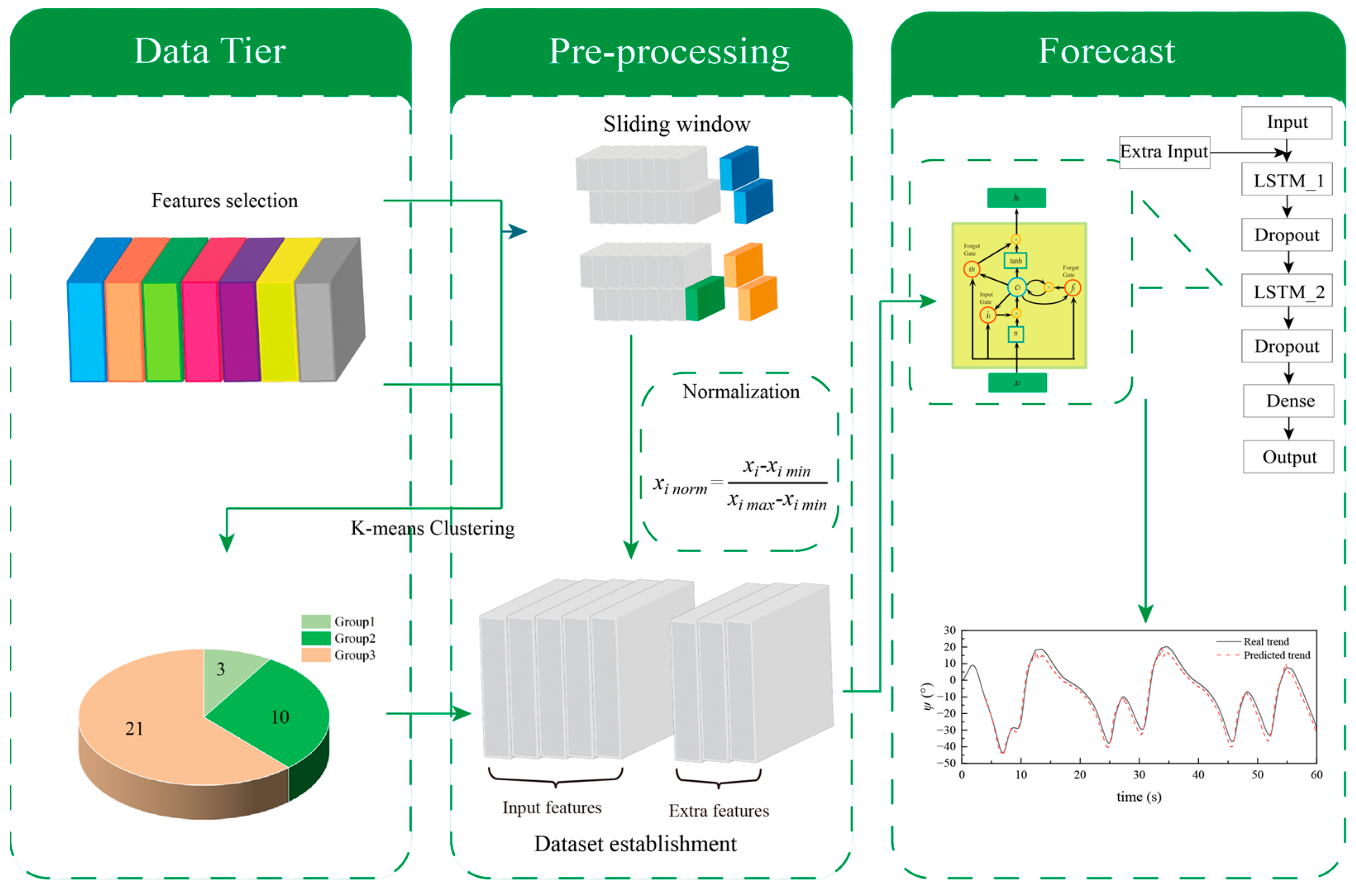
Figure 2.
Structure of LSTM.

Figure 3.
The data structure of LSTM.

Figure 4.
predicted by LSTM of different input lengths.


Figure 5.
Cluster analysis results.

Figure 6.
Comparison of the actual trend of each group after cluster analysis.

Figure 7.
predicted by LSTM of different training set.

Figure 8.
prediction results of Data6 and Data9.

Figure 9.
Prediction of all features.

Figure 10.
The comparison after removing each feature.


Figure 11.
predicted by LSTM using different numbers of datasets.
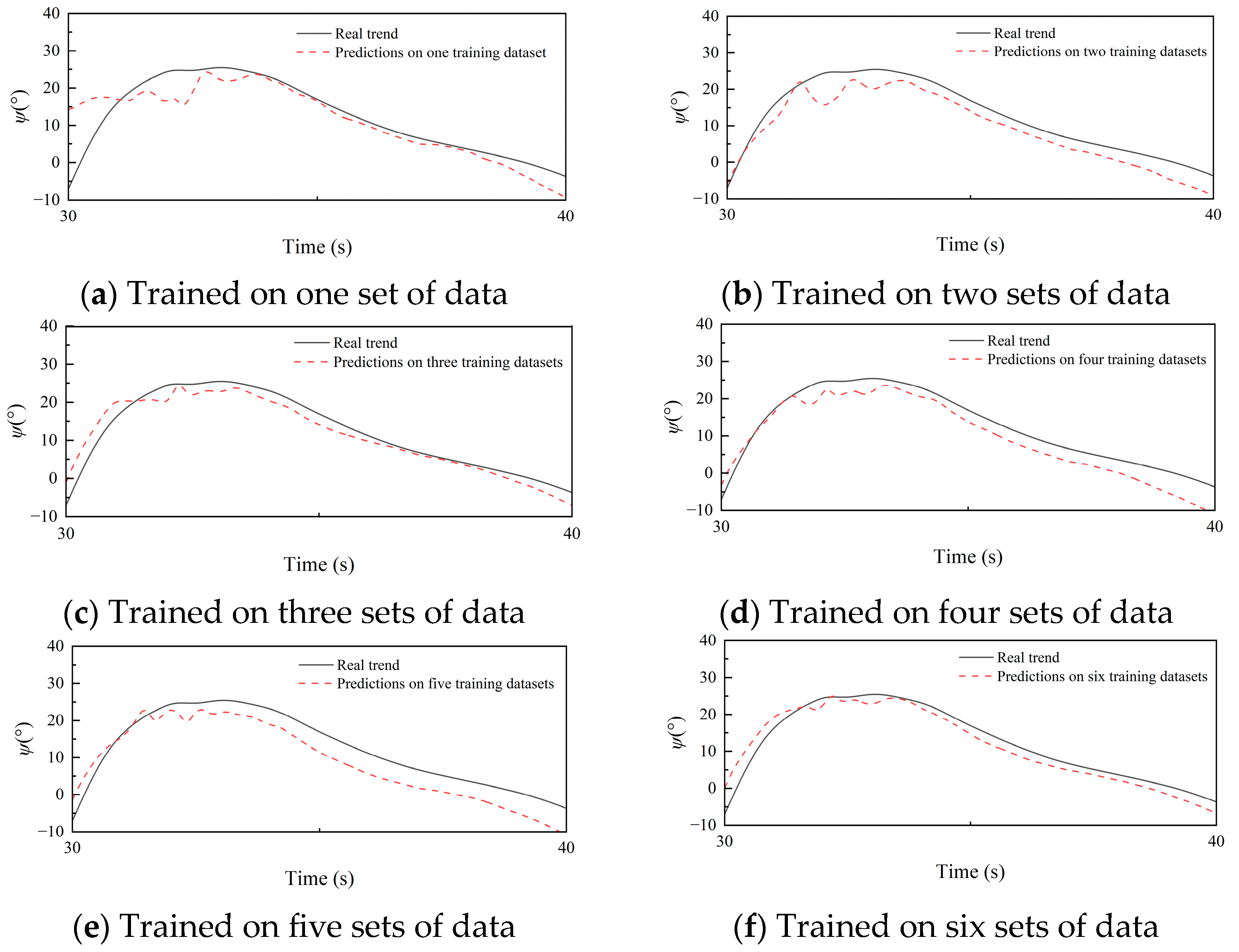
Figure 12.
Comparison of prediction of the optimized policy and the traditional policy.


Table 1.
Selected features for discussion.
| Classification | Initial Conditions | Heading | Wave | Trajectory | Speed | Motion | Force | Torque |
|---|---|---|---|---|---|---|---|---|
| Features | ||||||||
Table 2.
The structure and features of the neural network.
| Layers | Initial Values of Related Parameters |
|---|---|
| LSTM_1 | units: 50, return_ sequences: True predict_ step: 50 |
| Dropout_1 | rate: DROPOUT_RATE |
| LSTM_2 | units: 50 |
| Dense | units: TO BE DETERMINED |
| Activation | Relu |
| MinMaxScaler | feature_ range: (0, 1) |
| Train–Test Split | train_ ratio: 80%, test_ ratio: 20% |
| Time Step | time_ step: TO BE DETERMINED |
Table 3.
MAE, RMSE, and MAE for different input lengths.
| Input Length | MSE | RMSE | MAE |
|---|---|---|---|
| 250 | 101.13 | 10.05 | 3.30 |
| 500 | 76.93 | 8.77 | 3.00 |
| 750 | 96.77 | 9.83 | 3.35 |
| 1000 | 75.78 | 8.70 | 2.94 |
| 1500 | 84.44 | 9.18 | 3.26 |
Table 4.
MAE, RMSE, and MAE for different dataset.
| Dataset | |||
|---|---|---|---|
| Data1 | 0.91 | 0.38 | 5.45 |
| Data2 | 0.96 | 0.40 | 2.34 |
| Data3 | 1.08 | 0.45 | 2.24 |
| Data4 | 0.92 | 0.45 | 2.33 |
| Data5 | 1.08 | 0.45 | 3.27 |
| Data6 | 0.91 | 0.38 | 3.27 |
| Data7 | 1.32 | 0.55 | 5.45 |
| Data8 | 1.44 | 0.60 | 2.34 |
| Data9 | 1.13 | 0.35 | 2.34 |
Table 5.
MAE, RMSE, and MAE for datasets in different groups.
| Dataset Used for Training | MSE | RMSE | MAE |
|---|---|---|---|
| Data1 | 390.67 | 19.76 | 8.71 |
| Data2 | 301.30 | 17.35 | 8.39 |
| Data4 | 582.49 | 24.13 | 9.15 |
| Data7 | 1390.53 | 37.28 | 13.36 |
Table 6.
MAE, RMSE, and MAE of Data5 and Data8.
| Dataset Used for Training | MSE | RMSE | MAE |
|---|---|---|---|
| Data5 | 28.77 | 5.36 | 2.31 |
| Data8 | 505.40 | 22.48 | 8.39 |
Table 7.
Specific values for different initial conditions.
| Dataset | |||
|---|---|---|---|
| Training Data | 0.84 | 0.35 | 5.45 |
| Prediction Data | 1.08 | 0.45 | 2.24 |
Table 8.
MAE, RMSE, and MAE for different parameter combination.
| Removed Parameter | MSE | RMSE | MAE |
|---|---|---|---|
| - | 430.65 | 20.75 | 9.26 |
| Torque | 259.30 | 16.10 | 6.83 |
| Force | 235.77 | 15.35 | 5.60 |
| Motion | 465.37 | 21.57 | 9.56 |
| Speed | 483.63 | 21.99 | 9.89 |
| Trajectory | 474.67 | 21.78 | 10.13 |
| 422.28 | 20.54 | 8.69 |
Table 9.
Specific values for different initial conditions.
| Dataset | |||
|---|---|---|---|
| TrainingD1 | 1.24 | 0.35 | 2.34 |
| TrainingD2 | 0.84 | 0.35 | 5.45 |
| TrainingD3 | 0.84 | 0.35 | 3.27 |
| TrainingD4 | 0.84 | 0.35 | 2.34 |
| TrainingD5 | 0.91 | 0.38 | 5.45 |
| TrainingD6 | 1.18 | 0.45 | 2.33 |
Table 10.
MAE, RMSE, and MAE for different numbers of datasets.
| Number of Training Sets | MSE | RMSE | MAE |
|---|---|---|---|
| 1 | 2963.41 | 54.43 | 20.75 |
| 2 | 431.23 | 20.76 | 8.36 |
| 3 | 257.38 | 16.04 | 6.12 |
| 4 | 115.04 | 10.72 | 4.38 |
| 5 | 100.30 | 10.01 | 4.28 |
| 6 | 88.25 | 9.39 | 3.76 |
Table 11.
Specific values for different initial conditions.
| Dataset | |||
|---|---|---|---|
| TrainingD1 | 0.91 | 0.38 | 3.27 |
| TrainingD2 | 1.08 | 0.45 | 3.27 |
| TrainingD3 | 0.92 | 0.45 | 2.33 |
| TrainingD4 | 0.87 | 0.45 | 2.34 |
| TrainingD5 | 1.32 | 0.55 | 2.33 |
| TrainingD6 | 1.20 | 0.50 | 3.27 |
Table 12.
MAE, RMSE, and MAE for optimizing policy and traditional policy.
| Policy | MSE | RMSE | MAE |
|---|---|---|---|
| Traditional policy | 38.06 | 6.17 | 2.64 |
| Optimized policy | 31.76 | 4.94 | 2.30 |
Disclaimer/Publisher’s Note: The statements, opinions and data contained in all publications are solely those of the individual author(s) and contributor(s) and not of MDPI and/or the editor(s). MDPI and/or the editor(s) disclaim responsibility for any injury to people or property resulting from any ideas, methods, instructions or products referred to in the content. |
© 2023 by the authors. Licensee MDPI, Basel, Switzerland. This article is an open access article distributed under the terms and conditions of the Creative Commons Attribution (CC BY) license (https://creativecommons.org/licenses/by/4.0/).
Share and Cite
MDPI and ACS Style
Xu, J.; Gong, J.; Wang, L.; Li, Y. Integrating k-means Clustering and LSTM for Enhanced Ship Heading Prediction in Oblique Stern Wave. J. Mar. Sci. Eng. 2023, 11, 2185. https://doi.org/10.3390/jmse11112185
AMA Style
Xu J, Gong J, Wang L, Li Y. Integrating k-means Clustering and LSTM for Enhanced Ship Heading Prediction in Oblique Stern Wave. Journal of Marine Science and Engineering. 2023; 11(11):2185. https://doi.org/10.3390/jmse11112185
Chicago/Turabian StyleXu, Jinya, Jiaye Gong, Luyao Wang, and Yunbo Li. 2023. "Integrating k-means Clustering and LSTM for Enhanced Ship Heading Prediction in Oblique Stern Wave" Journal of Marine Science and Engineering 11, no. 11: 2185. https://doi.org/10.3390/jmse11112185
Note that from the first issue of 2016, this journal uses article numbers instead of page numbers. See further details here.