A Numerical Study on Modeling Ship Maneuvering Performance Using Twin Azimuth Thrusters

Abstract

A methodology of mathematical testing is proposed for a ship with twin azimuth thrusters based on numerical calculations. An unmanned surface vessel (USV) powered by two azimuth thrusters is considered, which is a model-scale configuration. The Ship Maneuvering Mathematical Model Group (MMG) model is introduced to describe forces on the hull and propellers. A set of captive tests (planar motion mechanism (PMM) and open-water tests) were simulated using STAR-CCM+ (16.06.008-R8) software to obtain hull hydrodynamic derivatives and azimuth thruster hydrodynamic coefficients. A maneuvering test of the model-scale ship with two azimuth thrusters is built based on numerical results, and numerical results are compared with the model-scale experimental data to validate the feasibility of numerical methods. The findings show that the usability of the developed mathematical test in predicting the maneuvering ability of ships with two azimuth thrusters is confirmed through numerical calculations.

1. Introduction

More and more ships are equipped with twin azimuth thrusters due to the requirement for better maneuverability. These ships are suitable for work in confined waters, such as rescue ships, off-shore vessels, supply ships, and cruisers. However, because ships are steered by azimuth thrusters, the maneuverability is obviously different from the conventional rudder and propeller-driven ship. At the same time, due to the obvious interaction between the two azimuth thrusters, the complex hydrodynamic effect, and the remarkable influence on ship maneuverability, the maneuvering capability and experimental method of the ships with azimuth thrusters are worthy of further study.

The methods of ship maneuverability research mainly include model-scale ship tests in a towing tank, full-scale ship tests, numerical simulation using computational fluid dynamics (CFD), and parameter identification based on application tests or full-scale ship data. At present, many methods based on theoretical calculation tests with experimental corrections are also widely used.

Alessandrini et al. [1] calculated the flow field and hydrodynamic force of a series 60 ship under oblique and rotary motions when considering the influence of free-plane waves. Tahara et al. [2] compared and analyzed the numerical results and the test value of the inclined shipping movement of the series 60 ship when the free-plane wave was considered and found that the two were in good agreement. Sakamoto et al. [3] numerically simulated the viscous flow field of DTM5415 with a complex hull surface in pure roll and pure yaw motion. While ignoring the influence of free surface, Yang Yong [4] carried out a numerical simulation on the pure transverse motion of the KVLCC1 ship test in deep and shallow water. Li Dongli [5] used the Ansys Fluent and dynamic grid technique to numerically simulate the hydrodynamic performance of a ship in pure roll and yaw motion and, proved the linear relationship between hydrodynamic force and motion frequency, and indirectly proved the feasibility of numerical simulation. The calculated results were consistent with those of the potential flow method. Zhou [6] carried out a numerical simulation of the viscous flow field around the ship in shallow water using the CFD method and obtained the variation law of the hydrodynamic coefficient under the influence of drift angle.

In recent years, more and more scholars have paid attention to the study of ships with azimuth thrusters. Islam et al. [7]. introduced a numerical prediction and experimental evaluation scheme for combined propellers. Delefortrie et al. [8] established a maneuvering motion test for an estuary container vessel with two interacting Z-drives by captive experiments in the towing tank. Based on the MMG test, Reichel et al. [9] obtained the hull hydrodynamic derivatives and pod propeller hydrodynamic coefficients of a medium-sized oil tanker through the captive test and open water test in the towing tank and verified them in the ship-handling simulator. Reichel et al. [10] researched the equivalent standard maneuvers for pod-driven ships by using the comparative test of two sister ships of the same scale brass tests, i.e., twin-pod and twin-propeller twin-rudder configurations. Mu et al. [11] established an MMG test for a small vector-propelled unmanned ship, “Lanxin”, by combining empirical formulas with system identification. Wu et al. [12] analyzed the forces acting on the twin azimuth propellers and established the MMG test to carry out the numerical simulation and prediction of the maneuverability and ascertain the hydrodynamic derivatives. The maneuverability of a self-propelled test ship with twin full-revolving rudder propellers was analyzed in a self-propelled test in still water and waves [13]. Luo [14] analyzed the influence of the pod structure on the hydrodynamic performance and the pod structure and hydrodynamic characteristics of the propellers through CFD. Ji [15] carried out the numerical simulation and prediction of the maneuverability of the ship with azimuth thrusters using the RANS method. Zhao et al. [16] predicted the self-propulsion performance of a ship with double-L-type podded propulsors and established a conversion method for the performance of a full-scale ship. Zhou et al. [17] verified and calculated the maneuverability prediction for a 27000 DWT multipurpose cargo ship. The results showed that the theoretical values are in good agreement with experimental results. Ruiz M T et al. [18] expounded a former test of an estuary vessel with two contra-rotating Z-drives and gave an extensive discussion of the effect of the Z-drives on the maneuvering behavior of the estuary vessel. Okuda et al. [19] used an equivalent single rudder (ESR) test to simulate the maneuvering of the ship with a twin-propeller and twin-rudder ship in shallow water, and the results showed that the theoretical values are in good agreement with the experimental results. Guillaume et al. [20] implemented a new mathematical model in the ship maneuvering simulator and compared it against free-running model tests, which, after slight tuning, seemed capable of capturing the maneuvering motion of the ship in 6DOF. Ghani et al. [21] compared the outcomes from experimental works on hulls with and without pods to describe the effect of pod propulsor attachment to the existing naval vessel hull form, which was designed for conventional propulsors in aspects of resistance and motion characteristics. Witold et al. [22] analyzed two different propulsion systems from the point of view of future control applications, one with a pushing single screw propeller and a blade rudder, the other with pods, and presented equations describing forces and moments generated in both systems, then showing exemplary results of a simulation in comparison to the real-time experiments for two ships. Chenliang Zhang et al. [23] yielded $X_{vv}$, $Y_v$, and $N_v$ of the ONRT hull at four advancing speeds via linear regression of the hydrodynamic forces and moments predicted by CFD calculations and concluded the relationship between hydrodynamic derivatives and advancing speed while giving the expressions of hydrodynamic derivatives that can be used in an MMG model.

Many of the above studies primarily focused on assessing the maneuverability of ships equipped with azimuth thrusters through towing tank tests. However, it is well known that towing tank tests are expensive, and most researchers lack the experimental conditions.

This study presents a method of maneuverability study for the ship with two azimuth thrusters using CFD numerical calculation. As a specific example, the captive test is conducted by numerical simulation on the STAR-CCM+ platform. In the present work, all calculations are based on the unsteady Reynolds-averaged Navier–Stokes (URANS) method and the shear stress transport (SST) k-w turbulence model. Maneuvering simulations of turning are conducted using the hydrodynamic coefficients obtained from numerical calculations. The test is validated by comparing the simulation results with the results of full-scale ship tests.

2. Methodology

2.1. Governing Equations

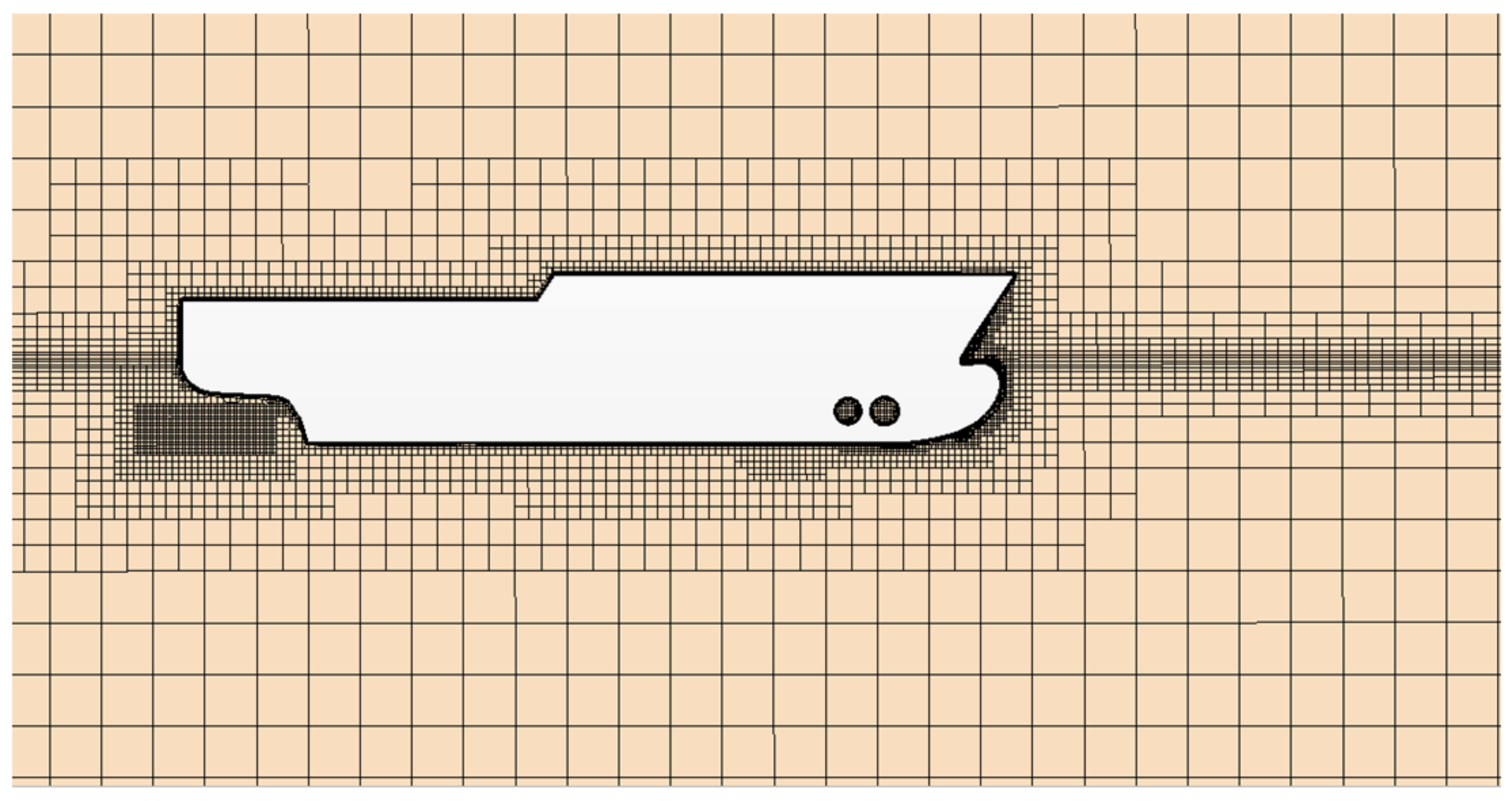
In this study, the RANS method was used to solve the flow field around the hull. Ship captive tests are conducted by planar motion mechanism (PPM). The PPM tests mainly consist of the simulation of oblique motion, pure sway motion, pure yaw motion, combined motions, and so on. The PMM tests are performed based on the simulation of the unmanned ships using the STAR-CCM+ platform, considering the influence of fluid viscosity and free surface wave profiles to calculate the hydrodynamic coefficients of the ship.

The governing equations include the continuity equation and momentum equation. The continuity equation is shown in the Equation (5) [12] as

$$\frac{\partial \rho }{\partial t}+\frac{\partial \left(\rho \left({\overline{u}}_i-u_{gi}\right)\right)}{\partial x_i}=0$$

(1)

The momentum equation is shown in the Equation (5) as

$$\frac{\partial \left(\rho {\overline{u}}_i\right)}{\partial t}+\frac{\partial \left(\rho {\overline{u}}_i\left({\overline{u}}_i-u_{gi}\right)\right)}{\partial x_i}=\frac{\partial }{\partial x_i}\left[\mu \frac{\partial {\overline{u}}_i}{\partial x_i}-\rho \overline{u_i^{\prime }{u}_j^{\prime }}\right]-\frac{\partial \overline{\rho }}{\partial x_i}+\rho f_i$$

(2)

where $\rho$ is the density of the fluid, ${\overline{u}}_i$ is the mean velocity of the fluid micro cluster in the i direction, $u_{gi}$ is the velocity of the grid cell in the i direction, $\overline{p}$ is the pressure, $f_i$ is the mass force, and $\rho \overline{u_i^{\prime }{u}_j^{\prime }}$ is the Reynolds stress, $i=1,2,3$.

The relationship between the Reynolds stress and the average velocity for incompressible fluid is established based on the Boussinesq assumption.

$$-\rho \overline{u_i^{\prime }{u}_j^{\prime }}={\mu }_t\left(\frac{\partial \overline{u_i}}{\partial x_j}+\frac{\partial \overline{u_j}}{\partial x_i}\right)-\frac{2}{3}\rho k{\varsigma }_{ij}$$

(3)

where ${\mu }_i$ is the turbulent dynamic viscosity coefficient, $k=\frac{1}{2}\left(\overline{u_1^{\prime 2}}+\overline{u_2^{\prime 2}}+\overline{u_3^{\prime 2}}\right)$ is the turbulent kinetic energy, ${\varsigma }_{\ddot{\upsilon }}$ is the second-order tensor of Kronecker isotropy, and the expression is as follows.

$${\zeta }_{ij}=\left\{\begin{array}{cc}1& i=j\\ 0& i\ne j\end{array}\right.$$

(4)

With the introduction of the relationship between Reynolds stress and mean velocity, the ten unknowns in the continuity equation and momentum equation are reduced to six, but the number of unknowns is still greater than the number of equations. Therefore, it is necessary to introduce a turbulence test to constitute a closed set of RANS equations.

2.2. Turbulence Model and VOF Method

The calculation accuracy of SST $k-\omega$ is the highest according to the commonly used turbulence tests and the previous calculation experience, mainly because the $k-\omega$ test has a good simulation effect on the low Reynolds number flow near the wall. The calculation results of $k-\epsilon$ are also good. The turbulence test takes the rotation effect into account and has good calculation results for low Reynolds number flow after treating the near-wall surface. Although the calculation accuracy of SST $k-\omega$ is higher than that of $k-\epsilon$, it takes more time, and it is difficult to achieve convergence because there is some rotating fluid in the large opening, and $k-\epsilon$ is very suitable for simulating complex fluid rotation problems. Therefore, the $k-\epsilon$ test is adopted. The $k-\epsilon$ turbulence model was used for the turbulence test, and the volume of fluid (VOF) method was used for the free surface capture solution.

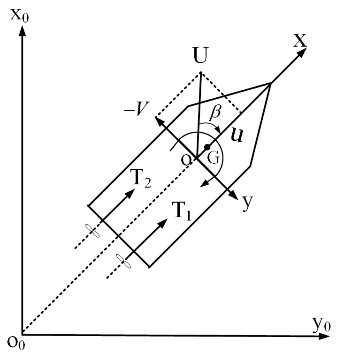
2.3. Coordinate System and MMG Test

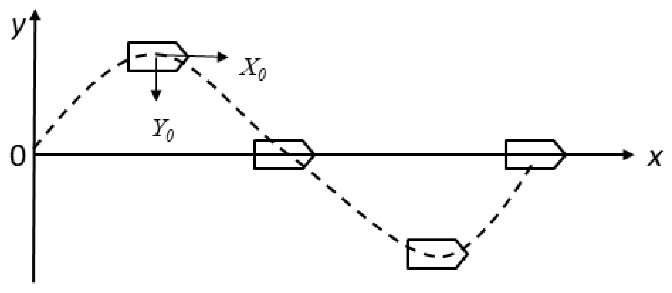
Figure 1 shows two right-hand cartesian coordinate systems used to establish MMG ship maneuvering motion models. One is the earth-fixed coordinate system, where the O₀-x₀-y₀ plane coincides with the still water surface, and the other is the horizontal ship-fixed coordinate system O-x-y, where O is the coordinate origin, which coincides with the gravity center of a ship.

It is assumed that the ship test is sailing in unrestricted deep and wide water. The ship is regarded as a rigid body, and the free surface is regarded as a still water surface. The present study only considers the motion of the ship in the horizontal plane and ignores the influence of the ship’s roll motion. Therefore, the mathematical test can be described by Equation (5) in the ship-fixed coordinate system.

$$\left\{\begin{array}{l}\left(m+m_x\right){\dot{u}}_r-\left(m+m_y\right){\upsilon }_{r}r=X_H+X_P\\ \left(m+m_y\right){\dot{\upsilon }}_r+\left(m+m_x\right)u_{r}r=Y_H+Y_P\\ \left(I_Z+J_Z\right)\dot{r}=N_H+N_P\end{array}\right.$$

(5)

where $m$ is the mass of the ship; $m_x$ and $m_y$ are the added masses for surge and sway; $I_Z$ and $J_Z$ are the moment of inertia and added moment of inertia for yaw, respectively; $u_r$ and ${\upsilon }_r$ are the surge and sway velocities, respectively; $r$ is yaw rate; $X_H$ and $X_p$, respectively, represent the forces acting in the longitudinal directions on the hull and propeller; $Y_H$ and $Y_P$, respectively, represent the forces acting in the lateral directions on the hull and propeller; $N_H$ and $N_P$ are the moments of the hull and propeller, respectively, with respect to the z-axis.

2.4. Forces and Moment Acting on the Hull

The principal aim of this study’s numerical simulations concerning a ship’s hull forces is to validate the applicability of the proposed methodology to vessels featuring dual azimuth thrusters. In situations where the numerical vessel model operates under conditions of slight motion and in a state of regular flow, the effect of higher-order terms in the equations is overshadowed by the prevailing impact of lower-order terms. Consequently, the omission of higher-order terms becomes justified. Furthermore, in scenarios characterized by regular flow conditions, such as calm water surfaces and constant flow velocities, the influence of higher-order terms in the equations on computational outcomes is relatively negligible, thus underscoring the feasibility of their simplification. Equation (6) [24] is used for the forces and moment acting on the hull.

$$\left\{\begin{array}{l}{X}_H\approx X_{u}u+X_{vv}{v}^2\\ Y_H\approx Y_v\nu +Y_{r}r\\ N_H\approx N_V\nu +N_{r}r\end{array}\right.$$

(6)

where $X_u$, $X_{vv}$, $Y_v$, $Y_r$, $N_V$, $N_r$ are the related hydrodynamic coefficients.

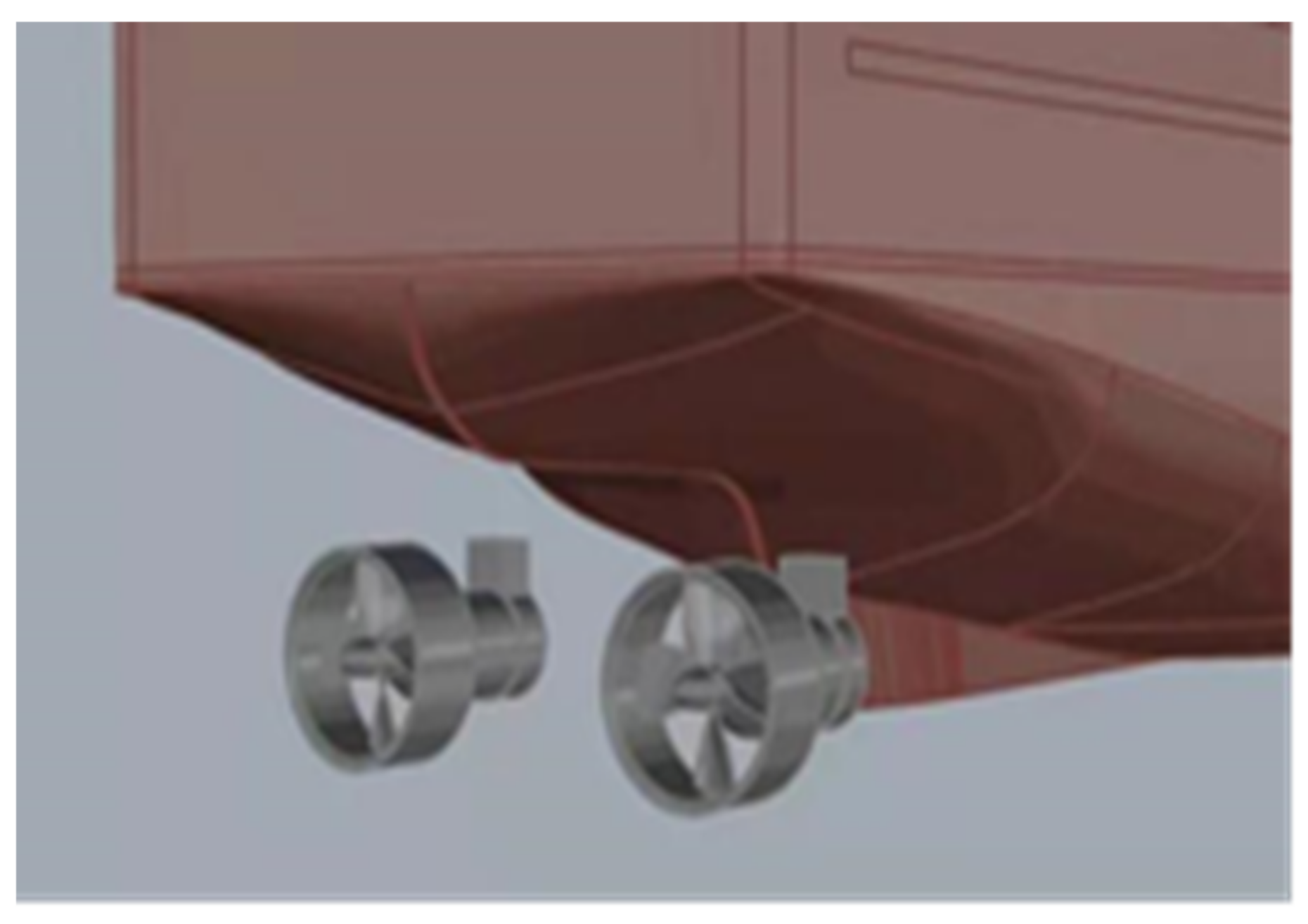
2.5. Forces and Moment Acting on Propulsors and Hull Interactions

The hydrodynamic characteristics of twin azimuth thrusters are highly intricate. Due to the independent maneuvering capability of these thrusters, they can be controlled either synchronously or asynchronously, resulting in a diverse range of deflection angle combinations. Consequently, considering the thrust distribution of dual azimuth thrusters, it is imperative to simultaneously account for both longitudinal and transverse forces. This paper primarily focuses on validating the feasibility of the numerical model’s performance and intends to conduct comprehensive investigations into the multidirectional hydrodynamic characteristics of dual thrusters in future studies. In this context, the present work offers a theoretical exposition of various factors influencing the azimuth thrusters, including the reciprocal influences between the vessel’s hull and the thrusters. The formulas are as follows:

$$\left\{\begin{array}{l}{X}_p=(1-t_p)X_{bhp}\\ Y_p=(1+a_h)Y_{bhp}\\ N_p=(x_p+a_h{x}_h)Y_{bhp}-y_p{X}_{bhp}\end{array}\right.$$

(7)

$$\left\{\begin{array}{l}{X}_{bhp}=T_{bhp}\cos \delta +S_{bhp}\sin \delta \\ Y_{bhp}=-T_{bhp}\sin \delta +S_{bhp}\cos \delta \end{array}\right.$$

(8)

$$T_{bhp}=\rho n^2{D}^4{K}_T({\alpha }_p,J_p)$$

(9)

$$S_{bhp}=\rho n^2{D}^4{K}_S({\alpha }_p,J_p)$$

(10)

where $X_{bhp}$, $Y_{bhp}$ are longitudinal and lateral force of propulsors for actual hydrodynamic conditions (behind hull propulsor), $t_p$ is the thrust coefficient, $a_H$ is the hull-propulsors interaction coefficient, $x_H$ is the location of additional lateral force induced on the hull by propulsors, $x_p$, $y_p$ are the coordinates of propulsors, $T_{bhp}$ is the thrust, $S_{bhp}$ is the side force on propulsors, $K_T$ is the thrust coefficient, $K_S$ is the side force coefficient, ${\alpha }_p$ is the actual water inflow to propulsors.

The relationship between the forces and moments exerted on the azimuth thrusters and the forces generated on the aft hull by the propeller is defined by Equation (7). The forces generated on the aft hull by the propeller are related to the propeller thrust, transverse force, and azimuth angle through Equation (8). However, it should be noted that the propeller thrust and transverse force are influenced by factors such as the actual inflow angle and advance coefficient of the propeller, as expressed in Equations (9) and (10). Equations (7)–(10) above are quotes from Maciej Reichel’s paper (2017) [9]. Consequently, the relationship between the actual inflow angle of the propeller and the propeller’s azimuth angle and drift angle can be experimentally determined to obtain the corresponding hydrodynamic coefficients using Equations (11) and (12).

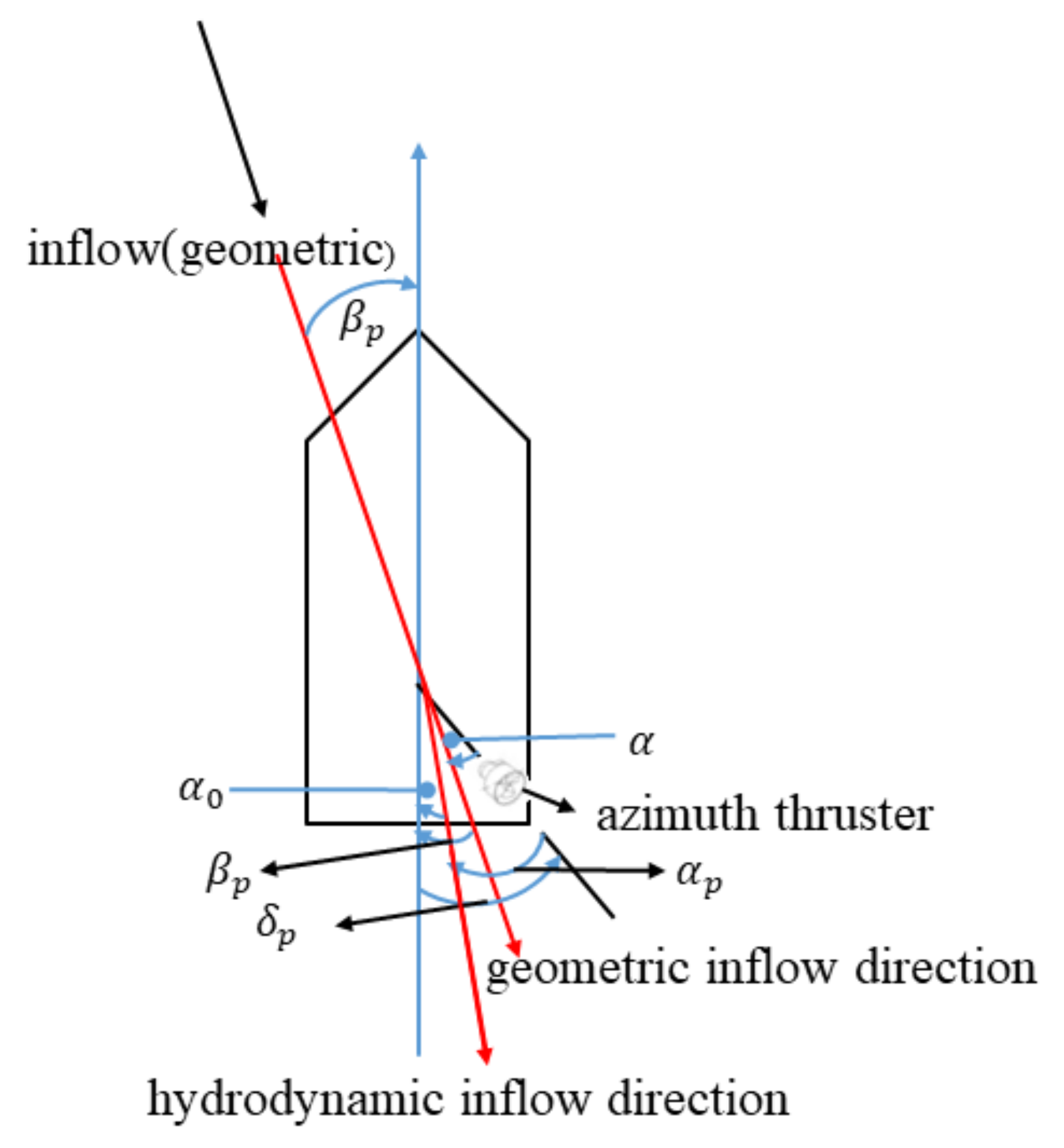
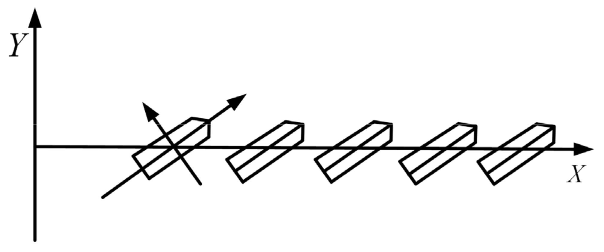
Figure 2 illustrates the relationship between the actual inflow angle of the propeller and the propeller’s azimuth angle and drift angle.

The relationships depicted in Figure 2 can be expressed as follows:

Geometric Azimuth Thruster Angle [24],

$$\alpha ={\delta }_p-{\beta }_p$$

(11)

Actual Water Inflow Angle,

$${\alpha }_p={\delta }_p-({\delta }_0+{\gamma }_p\beta )$$

(12)

where ${\delta }_p$ is the azimuth thruster angle relative to the longitudinal axis of the ship, ${\beta }_p$ is the geometric drift angle at the azimuth thruster, ${\beta }_p$ will be the same as the ship’s drift angle $\beta$ for oblique model tests, ${\delta }_0$ is the hydrodynamic neutral angle of propulsors, ${\gamma }_p$ is the flow straightening coefficient.

Consequently, utilizing the aforementioned series of equations, we can deduce the interrelationship between the propeller and the hull, as well as the correlation between the actual inflow angle of the propeller and the propeller’s azimuth angle. In our forthcoming investigations, we aim to ascertain the corresponding hydrodynamic coefficients by means of numerical simulations and experimental validation.

3. Numerical Setups and Verification

3.1. Study Model

In this study, an unmanned surface vessel (USV) called Smart Navigation 1 is the sample ship, which is owned by the Ship Intelligent Control Laboratory of Guangdong Ocean University. The ship is composed of an autonomous navigation system, an information collection system, and two azimuth thrusters driven by an electric system. In addition, the ship is also the model-scale ship of a novel rescue ship. The appearance of the ship is shown in Figure 3, and its principal parameters are listed in

Table 1. Principal parameters of the ship.

Principal Particular	Value	Unit
Length overall, Loa	1.90	m
Length between perpendiculars, L	1.80	m
Molded breadth, B	0.40	m
Molded depth, D	0.35	m
Designed draft, d	0.18	m
Displacement	95	kg
Vertical position of gravity center	0.2	m
Maximum speed	2.048	m/s
Design speed	1.278	m/s

.

The ship is equipped with twin azimuth propellers, shown in Figure 4 and Figure 5, and its main parameters are displayed in

Table 2. Propeller’s main parameters.

Principal Particular	Value
Diameter, DP (mm)	80
Blade no.	4
Pitch ratio, H/DP	1.4

.

3.2. Computational Model and Mesh Division

In this study, the six degrees of freedom (6DOF) motion of the hull was calculated by the dynamic fluid body interaction (DFBI) module. The overlapping grid technique was used to deal with the relative motion between the ship and the propeller and the large motion of the hull near the free liquid surface. The trimming mesh was chosen. It should be noted that the mesh division involves the free surface, and the refinement of the mesh should be carried out at the interface of water and air to ensure that the VOF method can be correctly used to capture the interface. For the maneuvering motion tests of virtual captive, such as simple yaw and simple sway motions, it should be noted that due to the active motion of the ship, the size of the fluid regions needs to be lengthened. For the active motion regions, mesh refinement should be carried out to ensure that the size is consistent with the overlapping mesh for better data transmission.

Figure 6 shows the mesh distribution around the hull and the free surface. To ensure the calculation accuracy and shorten the calculation time, the mesh on the waterline surface, bow, and stern was refined. The refined area at the waterline surface is consistent with the shape of Kelvin waves. For the regions far away from the hull, a relatively sparse mesh is used. The mesh size is 0.3% L. The surface size of the hull is 0.6% L, and the mesh size around the ship is 1.2% L. To improve the calculation accuracy of the free surface, it is necessary to refine the mesh of free surface, so the vertical mesh size of the free surface is 0.48% L and the horizontal mesh size of the free surface is 0.6% L.

The setting of the calculation regions and the mesh division of hull and drives is shown in Figure 7. To better simulate the boundary layer, the boundary layer grids are set around the hull, which has a great impact on the resistance calculation results. The number of boundary layers is six, and the y+ value varies between 30 and 300. The time step has a great influence on the stability and convergence of the calculation. It is ensured that the Courant number in most regions is less than one, while the Courant number in transient sensitive regions is less than 10, and the time step is 0.01 s.

3.3. Verification of Grid Independence

The quality of the grid directly affects the stability and precision of numerical calculation. The increase in the number of grids requires higher computing performance and longer computing cycles. Therefore, it is very important to select the appropriate mesh number to improve the precision of numerical calculation and shorten the calculation period. In this study, three different sets of grids were selected for grid independence verification: 2.27, 3.21, and 4.53 million. The calculation condition is a ship speed of 1.2 m/s. The results are shown in

Table 3. Grid independence verification.

Mesh Quantity/Million	Calculated Value/N	Experiment Value/N	Error
2.27	51.31	48.3	6.23%
3.21	49.55	48.3	2.59%
4.53	49.04	48.3	1.53%

, Error = 100% × (CFD − EFD)/EFD (in which the CFD is the Calculated Value, and the EFD is the Experiment Value). The grid convergence rate R_G is defined as R_G = (S₁ − S₂)/(S₂ − S₃), where S_i (i = 1, 2, 3) represents the results of resistance corresponding to the fine, medium, and coarse grids. |R_G| > 1 is divergence, −1 < |R_G| < 0 is oscillating convergence, and 0 < |R_G| < 1 is monotonic convergence. The results show that the calculation error of resistance is smaller, and the mesh size is more appropriate when the mesh size is 3.21 million. According to the formula, the convergence rate R_G of resistance can be obtained as 0.28, so the grid is judged to be monotone convergence. Therefore, considering the computational efficiency, 3.21 million grids were selected for subsequent calculation.

3.4. Oblique Motion Tests

The oblique motion of the ship is shown in Figure 8. The drift angle β of the test is fixed to be −12°, −8°, −4°, −2°, 0°, 2°, 4°, 8°, and 12°, respectively. The yaw rate r = 0, and the speed of the ship is 1.278 m/s. The motion can be described by Equations (13) and (14).

$$v=U\sin \beta$$

(13)

$$u=-U\cos \beta$$

(14)

where $u$ is the speed of the ship relative to the ground, and $\beta$ is the drift angle.

The hydrodynamic force $X_H$ in the longitudinal direction, the hydrodynamic force $Y_H$ in the lateral direction, and the yaw moment $N_H$ related to the drift angle are shown in

Table 4. The results of the oblique motion tests.

Speed (m/s)	β (°)	XH (N)	YH (N)	NH (N × m)
1.278	−12	11.3865	−13.3407	18.8779
1.278	−8	8.9124	−7.7792	13.5427
1.278	−4	7.8166	−5.2715	6.3455
1.278	−2	7.4267	−2.6313	3.2084
1.278	0	7.2500	0.0000	0.0000
1.278	2	7.3370	2.3582	3.0833
1.278	4	7.6619	5.0282	6.1467
1.278	8	8.7114	7.5912	13.4111
1.278	12	11.2877	13.1149	18.6955

.

Ship hydrodynamic equations in the oblique motion tests can be expressed as in Equations (15)–(17). Hull hydrodynamic coefficients are obtained by regressing and fitting data in

Table 5. Hydrodynamic coefficients by oblique motion tests.

Parameter	Value
Xu	48.26000
Xvv	78.48670
Yv	−56.02740
Yvvv	−223.62196
Nv	−83.49883
Nvvv	34.71836

. The hydrodynamic force and torque obtained through calculation are dimensionless transformed into:

$$X^{\prime }=\frac{X}{\frac{1}{2}\rho V^2{L}^2}$$

(15)

$$Y^{\prime }=\frac{Y}{\frac{1}{2}\rho V^2{L}^2}$$

(16)

$$N^{\prime }=\frac{N}{\frac{1}{2}\rho V^2{L}^3}$$

(17)

However, dimensionless coefficients are not used in this paper for the convenience of comparison with experiments. As shown in Figure 9, through data fitting using Matlab (R2021a), the following values can be obtained: $X_u$ = 48.26000, $X_{vv}$ = 78.48670, $Y_v$ = −56.02740, $Y_{vvv}$ = −223.62196, $N_v$ = −83.49883, and $N_{vvv}$ = 34.71836.

3.5. Pure Sway Test and Pure Yaw Test

Figure 10 depicts a pure sway test, while Figure 11 illustrates a pure yaw test. The ship is set at a certain speed $U$, the speed of swaying motion and yawing motion changes periodically. The drift angle $\beta$ is set to zero, and the motion can be described by Equations (18)–(22).

$$x=Ut$$

(18)

$$y=A\sin \omega t$$

(19)

$$\psi ={\psi }_0\cos \omega t$$

(20)

$$r=\dot{\psi }=-{\psi }_0\omega \sin \omega t$$

(21)

$$\dot{r}=\ddot{\psi }=-{\psi }_0{\omega }^2\cos \omega t$$

(22)

where ${\psi }_0$ is the heading change amplitude, and $A$ and $\omega$ are the amplitude and frequency of the simple harmonic oscillation, respectively. Generally, the yaw rate r is small, which can be described by Equation (23).

$${\psi }_0=\arctan \left(\frac{\omega y_0}{U}\right)$$

(23)

During the simulation, the speed U is fixed at 1.278 m/s in the x-axis direction, with the oscillation frequency $f=\omega /2\pi$ = 0.1 Hz in the y-axis direction, and the amplitudes are set to 0.12 m, 0.24 m, and 0.36 m, respectively. The results are presented in

Table 6. The results of the pure yaw motion tests.

Speed U (m/s)	F (HZ)	y0 (m)	XH (N)	YH (N)	NH (N × m)
1.278	0.1	0.12	10.80	2.38	4.57
1.278	0.1	0.24	10.89	4.82	9.08
1.278	0.1	0.36	10.82	6.59	13.62

.

The hydrodynamic equations in the yaw motion can be described in Equations (24) and (25), The results are presented in

Table 7. Hydrodynamic coefficients from the pure yaw motion tests.

Parameter	Value
$Y_r$	29.7577
$Y_{\dot{r}}$	3.2900
$Y_{rrr}$	−14.2470
$N_r$	62.7665
$N_{\dot{r}}$	7.0664
$N_{rrr}$	−29.6557

.

$$Y_H=Y_{r}r+Y_{\dot{r}}\dot{r}+Y_{rrr}{r}^3$$

(24)

$$N_H=N_{r}r+N_{\dot{r}}\dot{r}+N_{rrr}{r}^3$$

(25)

The force and moment variations over time during sway motion tests with amplitudes A = 0.5% L and A = 1% L can be observed in Figure 12 and Figure 13, respectively.

4. Results and Discussion

Through numerical simulations of oblique motion tests, pure sway tests, and pure yaw tests, we have obtained partial ship hydrodynamic coefficients. Furthermore, the added mass, moment of inertia, and proximity coefficient of the ship can be calculated, serving as valuable references for ship maneuvering experiments.

4.1. Added Masses Used for Maneuvering Test

The regression Equations (26)–(29) are used to calculate $m_x$, $m_y$, $I_z$ and $J_z$ of the ship.

$$\begin{array}{l}{m}_x=\frac{m}{100}\left[0.398+11.97C_B(1+3.73\frac{d}{B})+2.89C_B\right.\frac{L}{B}(1+1.13\frac{d}{B})\\ \left.+0.175C_B{(\frac{L}{B})}^2\times (1+0.54\frac{d}{B})-1.107\frac{L}{B}\times \frac{d}{B}\right]\end{array}$$

(26)

$$\begin{array}{l}{m}_y=m\left[0.882-0.54C_B(1-1.6\frac{d}{B})-0.156\times (1-0.673C_B)\frac{L}{B}\right.\\ \left.+0.826\frac{d}{B}\times \frac{L}{B}(1-0.678\frac{d}{B})-0.638C_B\frac{d}{B}\times \frac{L}{B}(1-0.669\frac{d}{B})\right]\end{array}$$

(27)

$$I_Z=m\times (0.35\times B{)}^2$$

(28)

$$J_Z=m{\left\{\frac{1}{100}\times \left[33-76.85\times C_B\times (1-0.784C_B)+3.43\times \frac{L}{B}(1-0.63C_B)\right]\right\}}^2$$

(29)

where $C_B$ refers to the block coefficient. The calculation results for the test ship are presented in

Table 8. Added masses for the tested ship.

Parameter	Value
$m_x$	−29.7491
$m_y$	70.9129
$I_z$	1.8620
$J_z$	2.8591

.

4.2. The Comparison of Numerical Simulation and Model-Scale Ship Test Results

The ship maneuvering motion test is determined as Equation (30) based on the parameters and coefficients obtained from the PMM tests and regression equations.

$$\left\{\begin{array}{l}65.2509\dot{u}-165.9129vr-78.4867v^2-48.28u=9.6777\times \\ \left({147.456\mathrm{K}}_T\left({\alpha }_P,J\right)\cos \delta +147.456K_S\left({\alpha }_P,J\right)\sin \delta \right)\\ 165.9129\dot{v}+65.2509ur+5.0274v-29.7577r=0.33152\times \\ \left({147.456\mathrm{K}}_T\left({\alpha }_P,J\right)\sin \delta +147.456K_S\left({\alpha }_P,J\right)\cos \delta \right)\\ 2.942\dot{r}-62.7665r+29.6557r^3=1.0680\times {10}^{-5}{n}^2\sin \delta \end{array}\right\}$$

(30)

The motion control equations of the vessel are also influenced by the advance speed J and the effective inflow angle α, the relevant aspects of which will be investigated in subsequent experiments.

Employing the maneuvering test, since there are multiple variables in Equation (30), the specific relationship between variables is given in the later study, and ${\alpha }_p\approx {\delta }_p$ is taken here for the simulation test. Equation (30) is reduced to:

$$\left\{\begin{array}{l}65.2509\dot{u}-165.9129vr-78.4867v^2-48.28u=9.8802\times {10}^{-6}{n}^2\cos \delta \\ 165.9129\dot{v}+65.2509ur-29.7577r-3.29\dot{r}+14.247r^3=3.3383\times {10}^{-6}{n}^2\sin \delta \\ 2.942\dot{r}-62.7665r+29.6557r^3=1.0680\times {10}^{-5}{n}^2\sin \delta \end{array}\right.$$

(31)

Numerical simulations are conducted in Matlab (R2021a), and the numerical results are compared with test results to validate the ship’s maneuvering tests. It has to be noted that additional external forces, including current, have not been taken into consideration during simulations.

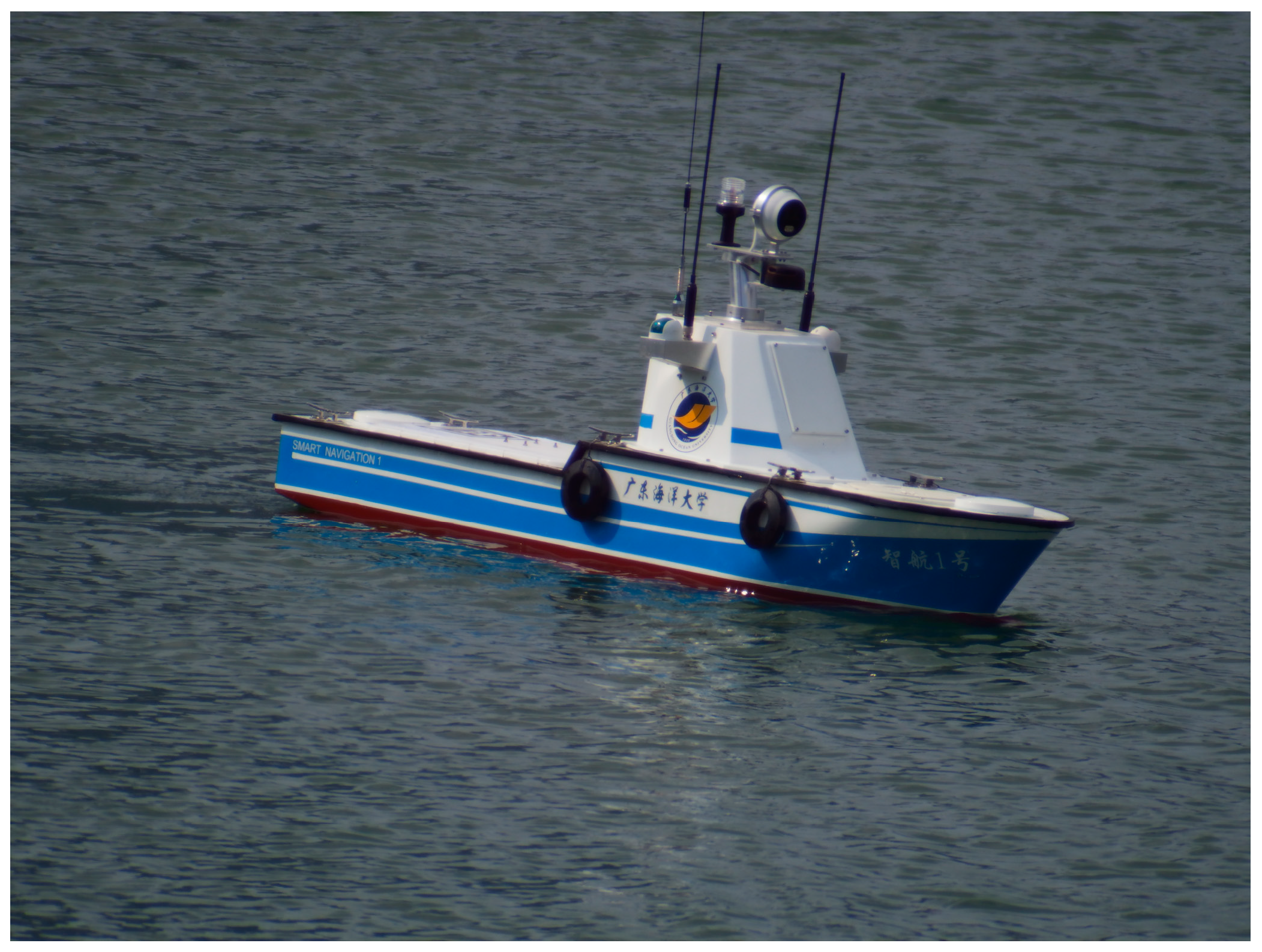
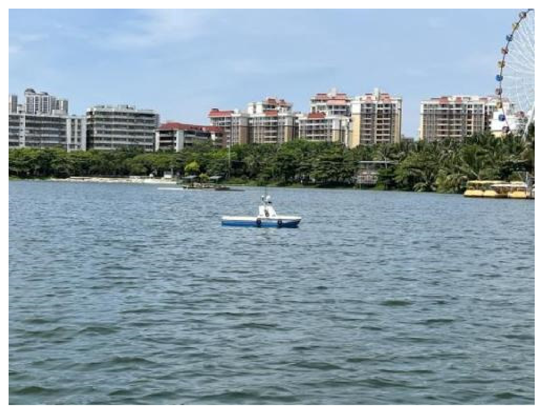
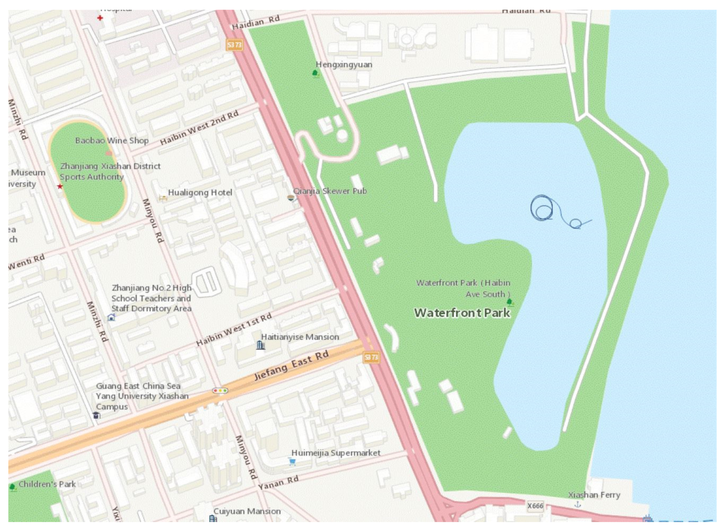
Model-scale ship tests were carried out on Moon Lake at Zhanjiang’s Haibin Park, shown in Figure 14. The turning tracks of the ship were derived from Google Maps, as shown in Figure 15. The wind velocity was around 2 m/s, and the wind direction was west during the tests.

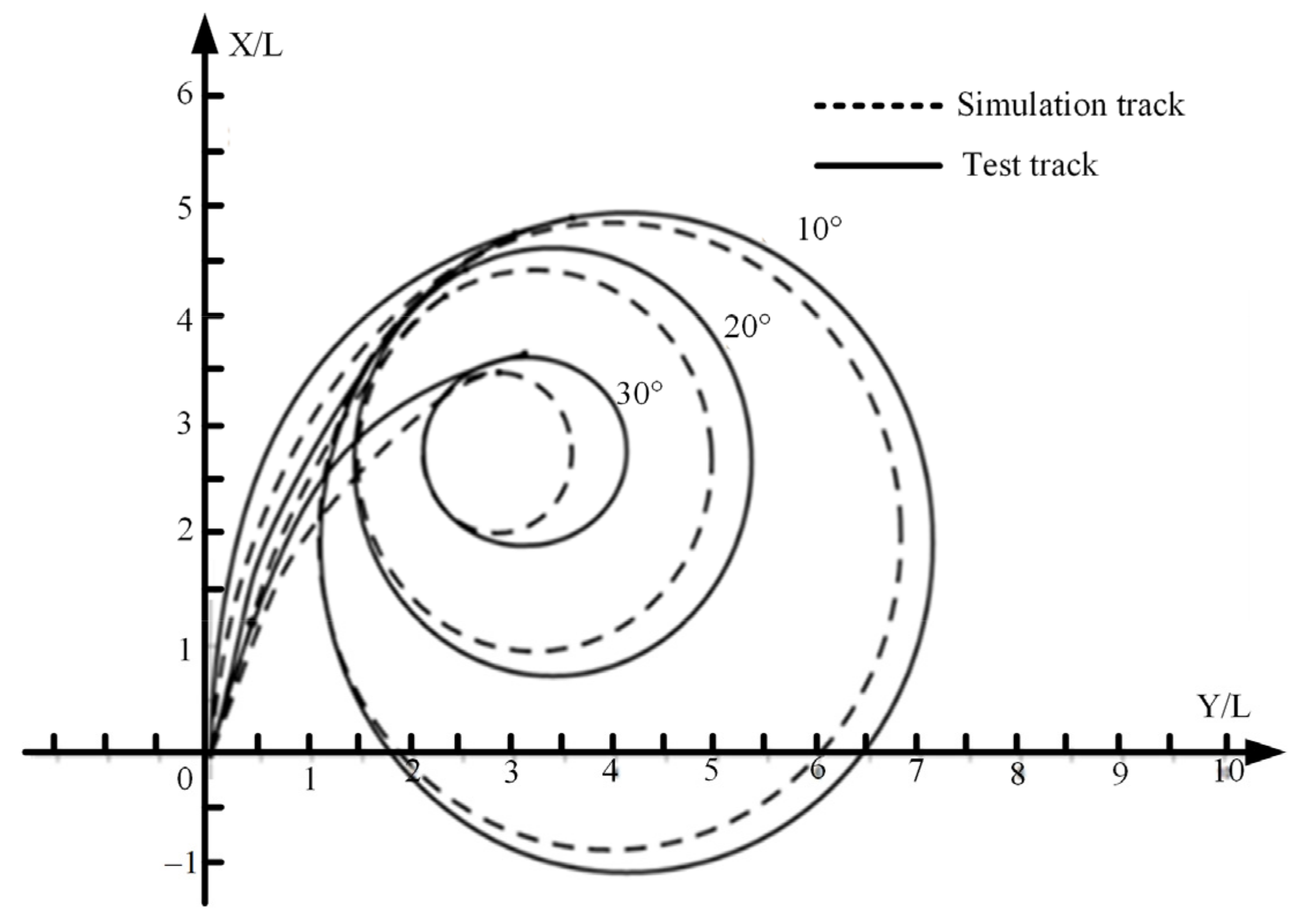
Model-scale ship tests were all conducted in unrestricted waters, without the interaction influence of shallow water or banks. It is worth noting that the twin propellers were kept at the same azimuth angles and revolutions.

Figure 16 shows the comparison between the numerical results and the experimental values of the 10°, 20°, and 30° starboard turning maneuvers. The simulation of the COG path shows smaller values of tactical diameter. The rate of turn from tests and simulations are similar and correspond well to each other. It can be seen that it is not possible to change the turning rate in a realistic time like simulations during test trials due to wind force. Nevertheless, the proposed mathematical test method can predict the ship's motion trend with acceptable accuracy.

5. Conclusions

In this study, a mathematical model was developed to predict the maneuvering abilities of a ship with twin azimuth thrusters. An approach to using the MMG test to describe forces and interactions on the hull and drives was introduced. To obtain hydrodynamic coefficients, including the hull hydrodynamic derivatives and azimuth propellers hydrodynamic coefficients, a set of captive tests of PMM and open-water tests were simulated using STAR-CCM+. The numerical results have been validated against test results. Based on the research conducted, the following conclusions can be drawn:

(1) The MMG approach can be successfully used in the case of ships with two azimuth thrusters, which can guarantee the description of the force of the ship with twin azimuth thrusters;

(2) STAR-CCM+ is a good tool for CFD numerical calculation to obtain hull hydrodynamic derivatives and the propeller’s hydrodynamic coefficients by simulating captive and open water tests, and the work can lower the cost compared with towing tank experiments;

(3) Although the developed and presented method for describing hydrodynamic characteristics of an azimuth thruster is simple, it has shown satisfactory precision and can be easily used in maneuvering prediction for this ship type;

(4) From the perspective of quantitative and maneuvering characteristics, the proposed mathematical test method can predict the trend of ship motion with acceptable accuracy.

However, it should be noted that the presented method has certain limitations. The ship’s model is currently designed based on the synchronous mode of two drives. In the near future, further research will be conducted to explore the ship’s model considering the asynchronous mode of two drives, which will take into account the interaction effects between the two drives.

References

1. Alessandrini, B.; Delhommeau, G. Viscous free surface flow past a ship in drift and in rotating motion. In Proceedings of the 22th Symposium on Naval Hydrodynamics, Washington, DC, USA, 9–14 August 1998. [Google Scholar]
2. Tahara, Y.; Longo, J.; Stern, F. Comparison of CFD and EFD for the Series 60 C B = 0.6 in steady drift motion. J. Mar. Sci. Technol. 2002, 7, 17–30. [Google Scholar] [CrossRef]
3. Sakamoto, N. URANS and DES Simulations of Static and Dynamic Maneuvering for Surface Combatant; University of Iowa: Iowa City, IA, USA, 2009. [Google Scholar]
4. Yang, Y.; Zou, Z.; Zhang, C. Numerical calculation of hydrodynamic dynamics of KVLCC hull in deep and shallow water. Res. Prog. Hydrodyn. 2011, 26, 85–93. [Google Scholar]
5. Li, D. Calculation of hydrodynamic derivative of ship maneuvering in viscous flow field. J. Harbin Eng. Univ. 2010, 31, 421–427. [Google Scholar]
6. Zhou, L. Numerical predictions of hydrodynamic forces on a ship during a low-speed drift motion in shallow water including verification and validation. J. Ship Mech. 2016, 20, 841–848. [Google Scholar]
7. Islam, M.F.; Veitch, B.; Liu, P. Experimental research on marine podded propulsors. J. Nav. Archit. Mar. 2007, 4, 57–71. [Google Scholar] [CrossRef]
8. Delefortrie, G.; Ruiz, M.T.; Vantorre, M. Maneuvering model of an estuary container vessel with two interacting Z-drives. J. Mar. Sci. Technol. 2018, 23, 739–753. [Google Scholar] [CrossRef]
9. Reichel, M. Prediction of Maneuvering abilities of 10000 DWT pod-driven coastal tanker. Ocean. Eng. 2017, 136, 201–208. [Google Scholar] [CrossRef]
10. Reichel, M. Equivalent standard manoeuvres for pod-driven ships. Ocean. Eng. 2019, 187, 106165. [Google Scholar] [CrossRef]
11. Mu, D.; Wang, G.; Fan, Y.; Sun, X.; Qiu, B. Modeling and Identification for Vector Propulsion of an Unmanned Surface Vehicle: Three Degrees of Freedom Model and Response Model. Sensors 2018, 18, 1889. [Google Scholar] [CrossRef] [PubMed]
12. Wu, X.; Gao, X. Maneuverability prediction for a ship with full-revolving twin propellers. Chin. J. Ship Res. 2017, 12, 27–31+62. [Google Scholar]
13. Wu, X.; Gao, X. Comparative Analysis on Model Test in Static Water and Waves for Full-revolving Propeller Boat. Ship Ocean. Eng. 2017, 46, 62–65. [Google Scholar]
14. Luo, X. Design of Full-rotating Podded Propeller and Study on the Characteristic of lts Hydrodynamics. Ship Eng. 2016, 38, 34–38. [Google Scholar]
15. Ji, X. Numerical Simulation and Analyzation of Ship Maneuvers with Azimuth Thrusters. Master’s Thesis, China Ship Research and Development Academy, Beijing, China, 16 January 2018. [Google Scholar]
16. Zhao, D.; Guo, C.; Lin, J.; Zhang, Z.; Bai, X. Prediction of Self-Propulsion Performance of Ship Model with Double L-Type Podded Propulsors and Conversion Method for Full-Scale Ship. J. Mar. Sci. Eng. 2019, 7, 165. [Google Scholar] [CrossRef]
17. Zhou, Z.; Sheng, Z.; Fen, W. On Manoeuvrability Prediction for Multipurpose Cargo Ship. Ship Eng. 1983, 6, 21–29+36+24. [Google Scholar]
18. Ruiz, M.T.; Delefortrie, G.; Vantorre, M.; Geerts, S. Propulsion and steering behaviour of a ship equipped with two contra-rotating Z-drives. In Proceedings of the 10th International Conference on Hydrodynamics, Saint Petersburg, Russia, 12 October 2012. [Google Scholar]
19. Okuda, R.; Yasukawa, H.; Sano, M.; Hirata, N.; Yoshimura, Y.; Furukawa, Y.; Matsuda, A. Maneuvering simulations of twin-propeller and twin-rudder ship in shallow water using equivalent single rudder model. J. Mar. Sci. Technol. 2022, 27, 948–970. [Google Scholar] [CrossRef]
20. Guillaume, D.; Marc, V. 6DOF manoeuvring model of KCS with full roll coupling. Ocean. Eng. 2021, 235, 109327. [Google Scholar]
21. Ghani, M.A.; Yaakob, O.; Ismail, N.; Kader, A.S.A.; Sabki, A.A.; Singaraveloo, P. Experimental analysis of podded propulsor on naval vessel. TransNav Int. J. Mar. Navig. Saf. Sea Transp. 2014, 8, 153–156. [Google Scholar]
22. Gierusz, W. Modelling the dynamics of ships with different propulsion systems for control purpose. Pol. Marit. Res. 2016, 23, 31–36. [Google Scholar] [CrossRef]
23. Zhang, C.; Liu, X.; Wan, D.; Wang, J. Experimental and numerical investigations of advancing speed effects on hydrodynamic derivatives in MMG model, part I: Xvv, Yv, Nv. Ocean. Eng. 2019, 179, 67–75. [Google Scholar] [CrossRef]
24. Molland, A.F.; Turnock, S.R. Flow straightening effects on a ship rudder due to upstream propeller and hull. Int. Shipbuild. Prog. 2002, 49, 195–214. [Google Scholar]
Figure 1. Coordinate system.
Jmse 11 02167 g001
Figure 2. The relationship graph between effective azimuth thrust angle and inflow angle.
Jmse 11 02167 g002
Figure 3. The ship Smart Navigation 1.
Jmse 11 02167 g003
Figure 4. A diagram of the propellers.
Jmse 11 02167 g004
Figure 5. The appearance of the propellers.
Jmse 11 02167 g005
Figure 6. Ship overlapping grid division.
Jmse 11 02167 g006
Figure 7. (a) The division of calculation regions. (b) The mesh division of hull surface. (c) The mesh division of propellers.
Jmse 11 02167 g007
Figure 8. Oblique motion tests.
Jmse 11 02167 g008
Figure 9. (a) Curve fitting for Y H . (b) Curve fitting for N H .
Jmse 11 02167 g009
Figure 10. Pure sway motion.
Jmse 11 02167 g010
Figure 11. Pure yaw motion.
Jmse 11 02167 g011
Figure 12. Graphs illustrating the temporal evolution of forces and moments (A = 0.5% L).
Jmse 11 02167 g012
Figure 13. Graphs illustrating the temporal evolution of forces and moments (A = 1% L).
Jmse 11 02167 g013
Figure 14. Moon Lake at Zhanjiang’s Haibin Park.
Jmse 11 02167 g014
Figure 15. Ship tracks in Google Maps.
Jmse 11 02167 g015
Figure 16. Starboard side turning circle trajectories.
Jmse 11 02167 g016