A Deep Learning-Based Lightweight Model for the Detection of Marine Fishes

Abstract

The species and population size of marine fish are important for maintaining the ecological environment and reflecting climate change. Traditional fish detection methods mainly rely on manual or traditional computer vision, which has disadvantages such as complex design, low detection accuracy, and poor generalization. The widespread use of ocean observation systems has accumulated a large number of images and videos, which makes the application of deep learning on marine fish detection possible. In this paper, a real-time high-precision fish detection algorithm based on YOLOv5s is constructed. Considering the enhancement of the channel representation and spatial interaction ability of the model, the attention mechanism and gated convolution are introduced, respectively, and GhostNet is introduced to lighten the model. Through a series of model comparisons, two improved models, S-Head-Ghost-Fish9 and S-SE-HorBlock-Head-Ghost-Fish9, are finally obtained. Compared with the original model, in terms of model size, the former reduces by 19% and the latter increases by 9.5%; in terms of computation, the former reduces by 15.7% and the latter reduces by 3.1%; in terms of detection speed, both take about 17 ms to detect a single image, and both can meet the real-time detection requirements; in terms of detection accuracy, the former improves by 3% and the latter by 3.6%. Compared with the latest detection algorithms of YOLOv6 and YOLOv8, the detection accuracy is slightly lower than 1%, but the model size and computation amount are only 1/3 to 1/2 of them. The improved models can help assess the population size and growth of the fish, which is of great significance in maintaining the stability of the fish population.

1. Introduction

The total area of the ocean is about 360 million square kilometers, accounting for 71% of the total area of the earth, and the ocean is rich in fish resources, which are of great value. Fish species and abundance can reflect the climate, and some researchers have found that changes in species in certain areas can be used as indicators of climate change. In addition, it can also reflect the ecological environment of the region to a certain extent [1]. In order to achieve sustainable economic development and maintain the entire marine ecological environment, it is necessary to conduct a certain assessment of the marine ecological environment.

The real-time detection of fish is the key to realizing the protection of marine fish resources. Obtaining information such as the species and number of fish in an image or video can help assess the population and growth of fish, which is of great significance for maintaining the stability of the fish population [2]. However, it is unrealistic to rely on humans to manually analyze these images and video data, which is time-consuming, labor-intensive, and prone to errors. We urgently need to rely on computer vision to help us analyze these data automatically.

In this paper, we conduct fish object detection based on marine fish images. During this process, we first locate the position of the fish targets in the images and then further categorize the species of the fish targets. Fish detection can be categorized into two main categories, based on traditional computer vision and based on deep learning. Most of the traditional computer vision methods use hand-designed operators to extract fish features, and different operators need to be designed for different categories of fish, which generally has the disadvantages of complex detection and poor generalization. In addition to this, in the recognition process, it is also susceptible to the interference of environmental factors, such as light, background, etc., and there are problems such as difficulty in feature extraction and poor robustness.

Hsiao et al. [3] proposed a fish recognition and localization method relying on local ranking and maximum probability based on sparse representation classification, which was trained on a dataset covering 25 fish species with a total of 1000 images, and achieved a recognition accuracy of 81.8% and a localization accuracy of up to 96%. However, the pixels of each image were only $180\times 130$, which could not guarantee accuracy on high-pixel images. Cutter et al. 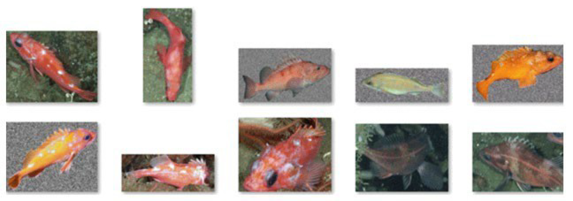[4] constructed an automatic fish detection method based on a cascade classifier of Haar-like features to recognize rockfish and their related species in a complex seabed rocky background, and the accuracy could reach 89%, but it was susceptible to the orientation of the fish, the distance, and the intensity of the light. Mehdi et al. [5] proposed a shape-based fish detection, which first obtained the shape features of the related fish by Principal Component Analysis (PCA) method and then located the feature points by Hal’s classifier, which could overcome some of the background disturbances in the underwater environment test. Aiadi et al. [6] proposed a lightweight network, namely MDFNet, for ear description. This method mentioned the concept of a lightweight model, but the network used was still based on traditional computer vision methods with limited feature extraction capability of the model.

Thanks to the continuous development of graphics processors, deep learning is widely used in many fields such as autonomous driving, medical imaging, smart agriculture, and security monitoring. For example, Khasawneh et al. [7] used faster R-CNN and deep transfer learning to realize the detection of K-complexes in EEG waveform images. Convolutional neural networks can perform feature learning and hierarchical feature extraction with efficient algorithms. which can provide better representations of images and learn these representations from large-scale data, with better generalization performance compared to traditional approaches.

In 2015, Li et al. [8] utilized Faster R-CNN to detect fish and tested it on the ImageCLEF dataset, which contained a total of 24,277 images of fish in 12 classes, and the mAP reached 0.814, which was an improvement of 11.2% compared to the previous approach, and the detection speed was close to 80 times faster. However, compared to the later proposed one-stage detection model, the two-stage detection model still has shortcomings in detection speed, and there is much room for improvement in detection accuracy. In 2017, Sung et al. [9] used YOLOv1 to detect seaweed, rocks, and fish on the seabed with a dataset that included a total of 1912 images, with an accuracy of 93% and a frame rate of 16.7 frames per second. However, due to the small sample dataset, early YOLOv1 generated only two prediction frames per grid and only one class, which resulted in poor performance for dense object detection. In 2018, Miyazono et al. [10] proposed a feature-point representation method, called annotated image, by adding four feature points (mouth, dorsal fin, caudal fin, and anal fin) to each fish image and performed it on AlexNet training, and its accuracy could reach 71.1% but there were fewer than 20 images in each category, which affected the training performance of the model. In addition, the annotation of the images was relatively complex and cumbersome, which also added workload to the target detection task. In 2018, Xu et al. [11] applied deep learning to hydroelectricity for the first time and used stochastic gradient descent and Adam’s optimizer to train the improved YOLOv3 to recognize fish near hydroelectricity, and the average mAP on three datasets reached 0.539. This work applied fish detection to the field of hydroelectricity, which is of great significance, but further improvement is still needed in the detection accuracy of the improved model. In 2020, Cai et al. [12] constructed a total of 2000 fish images and utilized MobileNetv1 as a feature extraction network in combination with YOLOv3 training to detect fish in a real fishing environment, with a mAP as high as 0.796. The result showed that the model had missed detections and lacked competitiveness in detection accuracy. In 2021, Zhao et al. [13] addressed the complex underwater environments for fish recognition and localization in complex underwater environments; they improved the Residual Network (ResNet) to enhance the feature extraction ability of the network and also designed the Enhanced Path Aggregation Network (EPANet) to solve the problem of low utilization of semantic information due to linear up-sampling, with an mAP as high as 0.928. This study showed good performance in detection accuracy, and further research could be conducted on the lightweight model in the future. In 2022, Connolly et al. [14] constructed the acoustic image dataset and compared it from three aspects, which were direct acoustic images, acoustic images with shadows, and the combination of the previous two. The experimental results showed that the F1 score was up to 0.9. The introduction of acoustic images provided a new idea for fish detection but this method could not achieve detection for specific fish species.

Deep learning has been widely used in various fields since it was proposed. In recent years, various deep-sea observing systems have been widely used in ocean monitoring, providing a large number of information-rich underwater videos and images, which makes the application of deep learning on marine fish detection possible; however, at the same time, it still faces the problems of poor quality datasets and insufficiently advanced detection algorithms; this paper will address the above problems.

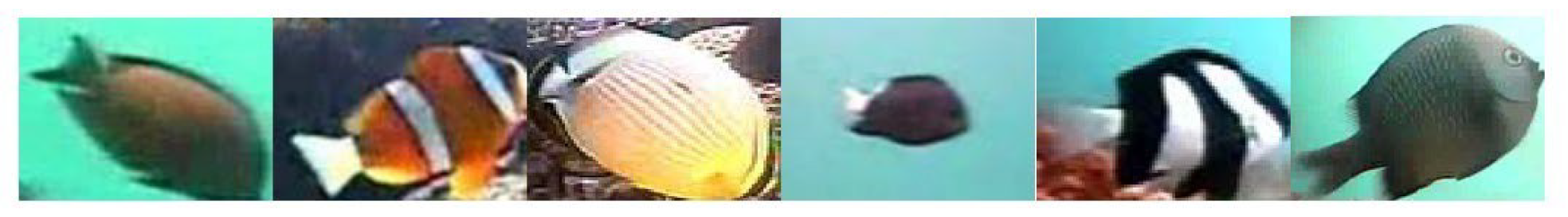
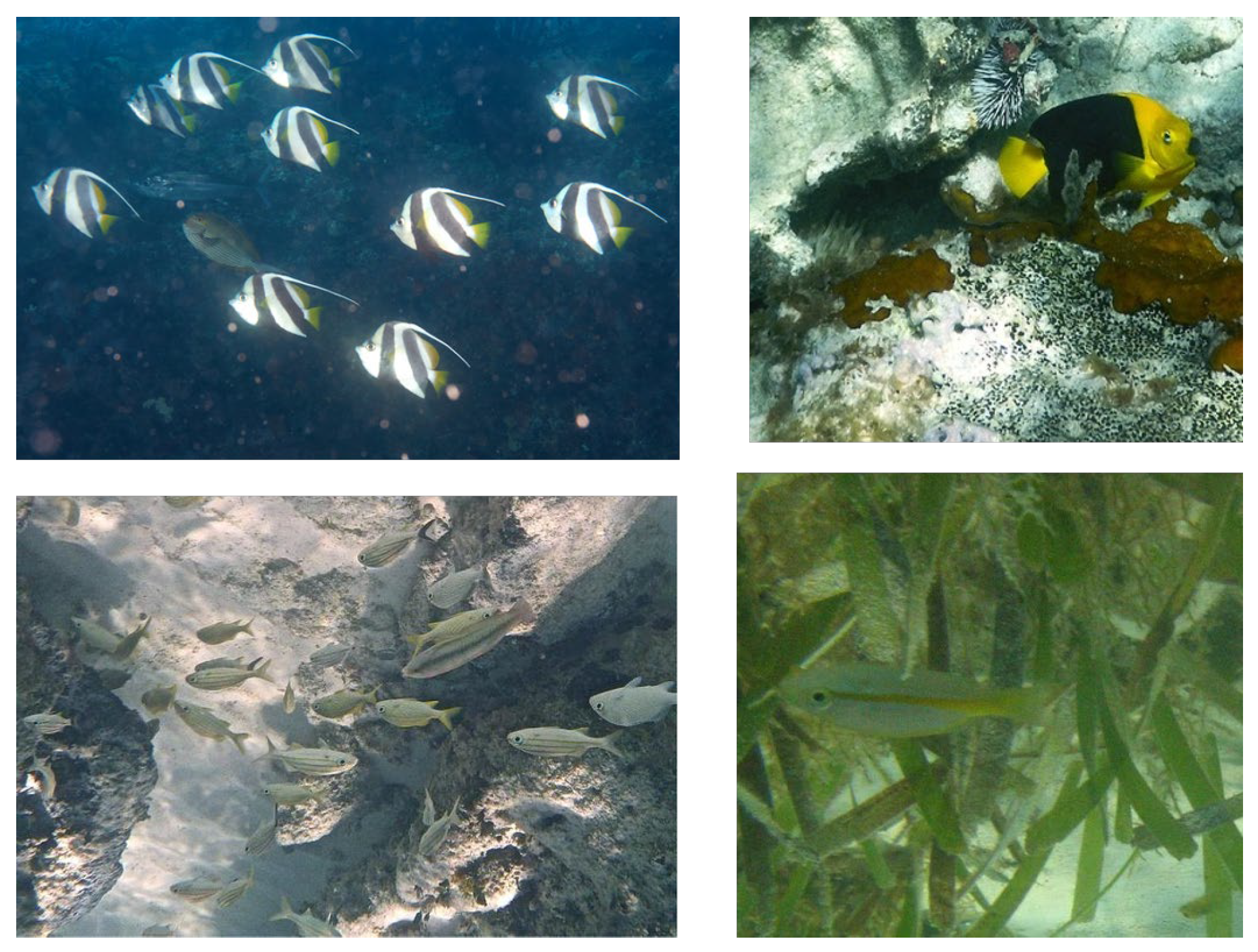
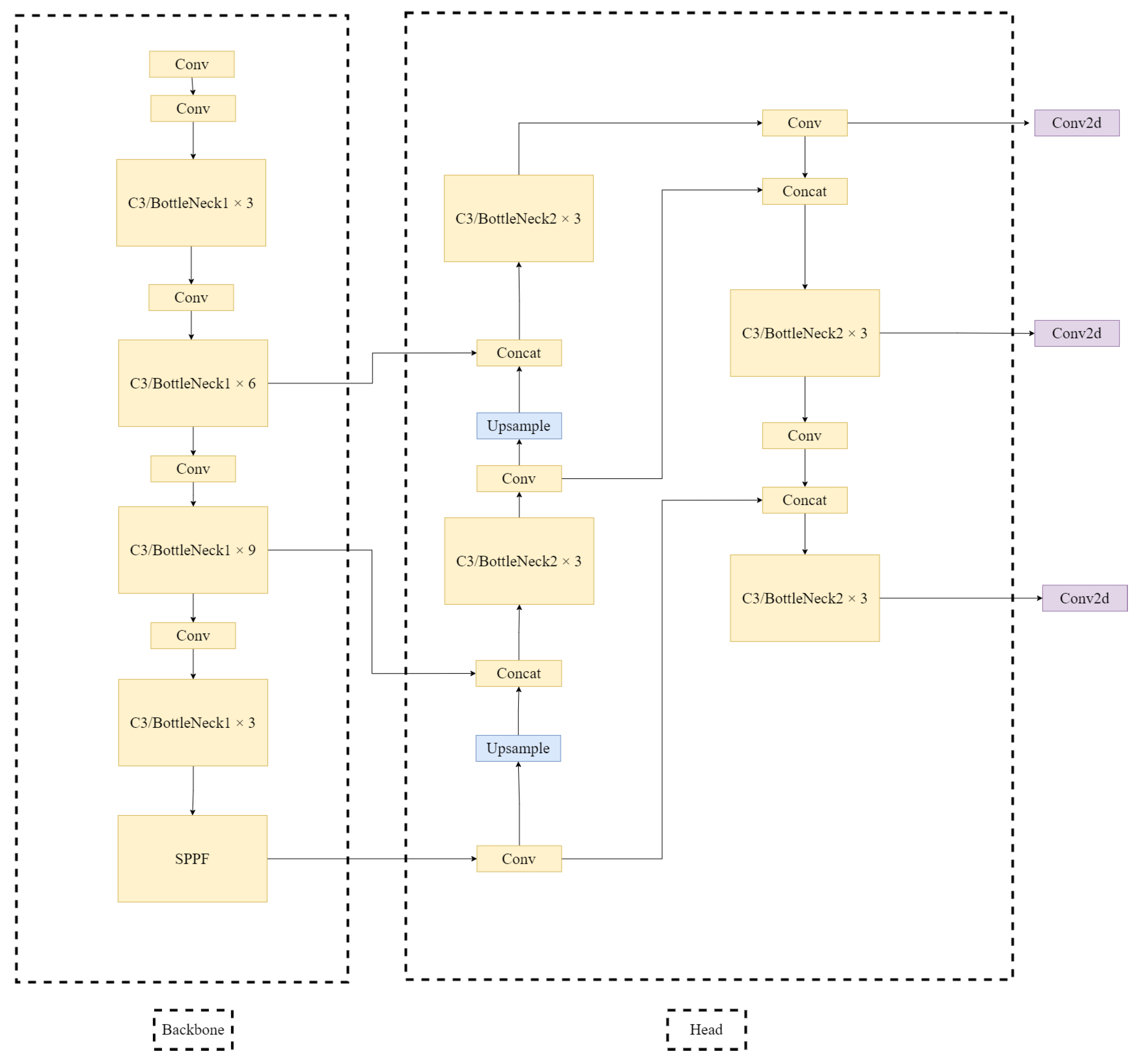
In this paper, we focused on fish near coral reefs as the research object, constructed a high-quality marine fish dataset, and optimized the detection performance of the model based on the existing deep learning of previous researchers to realize the detection of marine fish. The main contributions of this paper are as follows: (1) We constructed the Fish9 marine fish dataset by crawling high-definition coral reef fish images on the web, which can satisfy the research of this paper and provide data support for other related studies at the same time. (2) We introduced migration learning, attention mechanism, gated convolution, and GhostNet to the original YOLOv5s model to improve its detection performance while lightweighting the model. The experimental results showed that the improved model reduces the model size by 19% while improving the detection accuracy by 3%.

The rest of this paper is organized as follows. The second part introduces the improvement methods and ideas used in this article, and the third part presents a series of ablation experiments and their results and analyzes and discusses the improved algorithm proposed in this article based on the experimental results. The fourth part summarizes the work performed in this article.

2. Materials and Methods

2.1. Construction of the Dataset

Common ocean datasets include Fish4knowledge, Labeled Fishes in the Wild, Rockfish, ImageCLEF, and more. However, most of these datasets have low-quality images, blurred backgrounds, lack of images of complex scenes, and extremely unbalanced positive and negative samples. A few common datasets are shown in Figure 1, Figure 2 and Figure 3.

The above datasets have the disadvantages of low-quality, unbalanced categories, poor image clarity, and single image backgrounds. Aiming at the above problems, in this paper, we obtained the original fish dataset by means of online crawler in order to ensure the balance of the categories and image clarity and, at the same time, considering the richness of the fish background, we handpicked 9 types of fish images of the original fish dataset [15]. At the same time, we carried out a certain expansion by means of data enhancement to obtain the final dataset, Fish9, of which the training set and the test set are divided into a ratio of 9:1.

Some fish images in the Fish9 dataset are shown in Figure 4.

The categories and quantities of the final dataset are shown in

Table 1. Fish9 data set.

Category	Quantities
Angelfish	2772
Blennies	2399
Butterflyfish	3576
Gobies	2244
Grouper	2904
Grunt	2496
Snappers	2412
Surgeonfish	3204
Triggerfish	2232
Sum	24,239

. Among them, the number of Angelfish is 2772, Blennies is 2399, Butterflyfish is 3576, Gobies is 2244, Grouper is 2904, Grunt is 2496, Snappers is 2412, Surgeonfish is 3204, and Triggerfish is 2232, totaling 24,239 images. Its data volume can preliminarily meet the data scale required for general network training.

2.2. Object Detection Algorithm Based on YOLOv5

YOLOv5 is a one-stage algorithm, i.e., localization and classification are performed by a single network, and no additional networks are needed. YOLOv5 was proposed by Ultralytics and improved upon YOLOv4. There are a total of five versions of the YOLO family of algorithms [16,17,18,19]. YOLOv5 combines the advantages of the previous versions and other networks in the same period and strikes a good balance between the accuracy of the network and the speed of inference. In the Backbone part, YOLOv5 uses the CSPDarknet53 Backbone network, which is relatively lightweight to minimize computation and memory usage while ensuring high detection accuracy. In the neck part, YOLOv5 introduces multi-scale prediction, while utilizing Feature Pyramid Network (FPN) [20] and Path Aggregation Network for Instance Segmentation (PANet) [21]. The FPN is responsible for transferring deep semantic features to the shallow layer and enhancing semantic representation at multiple scales, while the PANet transfers shallow localization information to the deep layer and enhances localization capability at multiple scales. YOLOv5 enhances semantic representation and localization capability at multiple scales through the combination of these two modules. In the head part, the main part of which is three detectors, i.e., the process of object detection on feature maps of different scales using grid-based anchors. Finally, the network outputs three feature maps of different sizes obtained from the neck part, specifically the 17th, 20th, and 23rd layers of the network, representing shallow features, medium features, and deep features. With different sizes of feature maps, the target objects are detected in small, medium, and large scales, which greatly reduces the mistake of misdetection. The structure of YOLOv5 is illustrated in the following Figure 5.

YOLOv5 utilizes two variables, depth multiplier and width multiplier, to control the depth and width of the network. The number of input channels for each version is shown in

Table 2. Comparison of the number of output channels of different versions of YOLOv5.

Model Version	Layer1 Output	Layer2 Output	Layer4 Output	Layer6 Output
n	16	32	64	128
s	32	64	128	256
m	48	96	192	384
l	64	128	256	512
x	80	160	320	640

below. Too few input channels result in too little information extraction, while too many input channels result in a very large network model.

Meanwhile, YOLOv5 proposes a series of techniques to speed up the inference speed of the model, such as the adaptive image scaling technique called Letterbox. In object detection, the size of the input image varies, and, generally, in order to achieve better detection results, the size of the input network will be uniformly scaled to the same size. The general approach is to resize the input images. However, the aspect ratio of different images is not the same, which can easily cause the loss of image information. The authors of YOLOv5 took this into account and proposed the Letterbox adaptive image scaling technique.

The main idea of Letterbox is to utilize the information features of the network receptive field as much as possible while minimizing the size of image filling as much as possible. In YOLOv5, the commonly used network size is 416 × 416, 608 × 608, and so on. If there is an 800 × 600 picture input, it needs to be scaled to 416 × 416. The specific implementation is to choose the minimum value of the aspect scaling amount. The length scaling factor is 416/800 = 0.52, while the width scaling factor is 416/600 = 0.69. Therefore, choose 0.52 as the scaling factor, and at the same time, multiply the original picture by the scaling factor to obtain the scaled size of 416 × 312. It is worth noting that, there are 5 times of downsampling of YOLOv5, so the size of the picture is a multiple of 32, which is more conducive to the calculation. This is shown by pixel padding the width 312 to a multiple of 32, resulting in a final size of 416 × 320. This ensures the original aspect ratio and the least number of pixels to be padded, which can speed up the inference without losing the semantic information of the image.

2.3. Attention Mechanisms Study

In order to improve the representation ability of the model, one can consider correcting features by modeling the relationship between channels, thus enhancing useful features and diluting useless ones. SENet (Squeeze and Excitation) [22] is a plug and play attention mechanism module that allows networks to better focus on useful information, redistribute weights between channels, and significantly improve network performance while only increasing a small amount of computation. The structure of the SE module is shown in Figure 6.

For input $x\in R^{H^{{}^{\prime }}\times W^{{}^{\prime }}\times C^{{}^{\prime }}}$, where $F_{tr}$ stands for the ordinary convolution operation, the output $U\in R^{H\times W\times C}$ is obtained after the convolution operation. In general, U can be represented as $U=\left[u_1,u_2,\dots ,u_C\right]$, where $u_i$ denotes the i th 2D matrix of the feature layer. $F_{sq}$ represents the compression operation with input $U\in R^{H\times W\times C}$ and output $z\in R^{1\times 1\times C}$. In general, each point in the feature map obtained by convolutional kernel computation has a corresponding receptive field, and only information within that receptive field can be utilized. As the network deepens, the receptive field gradually expands, but the receptive field of the network in the previous layers is often very small. To solve this problem, we can compress the global spatial information into the channel dimension by using global pooling. Specifically, for the cth component of z, this can be expressed as Equation (1).

$$z_c=F_{sq}\left(u_c\right)=\frac{1}{H\times W}\sum _{i=1}^H\sum _{j=1}^W{u}_c\left(i,j\right)$$

(1)

In order to obtain the correlation between the channels, the weights of each channel will be calculated next using the excitation module $F_{ex}$, whose output s can be expressed as Equation (2):

$$s=F_{ex}\left(z,W\right)=\sigma \left(g\left(z,W\right)\right)=\sigma \left(W_2\delta \left(W_{1}z\right)\right),$$

(2)

where $W_1$ and $W_2$ are fully connected layers with dimensions $\frac{C}{r}\times C$ and $C\times \frac{C}{r}$, respectively, and r is a scaling parameter, which is generally taken as 16. For the output z of the compression module, the first step is to pass through the $W_1$ output with a dimension of $1\times 1\times \frac{C}{r}$; $\delta$ stands for the ReLU activation function, and the dimension remains unchanged after the ReLU activation function and then passes through the $W_2$ output with a dimension of $1\times 1\times C$, and $\sigma$ stands for the sigmoid activation function. After the sigmoid activation function, the output s is obtained with a dimension of $1\times 1\times C$. The last step is used to adjust the channel weights of the inputs, and the final output $\stackrel{\sim }{x}$ can be expressed as $\stackrel{\sim }{x}=\left[{\stackrel{\sim }{x}}_1,{\stackrel{\sim }{x}}_2,\dots {\stackrel{\sim }{x}}_c\right]$, and the cth component ${\stackrel{\sim }{x}}_c$ can be expressed as Equation (3):

$${\stackrel{\sim }{x}}_c=F_{scale}\left(u_c,s_c\right)=s_c·u_c,$$

(3)

where $F_{scale}$ is a dot multiplication operation and $u_c$ represents the cth component of the previous output $U=\left[u_1,u_2,\dots ,u_C\right]$.

2.4. Gated Convolutional Study

In order to improve the modeling capability of the model, this paper considers the introduction of gated convolution [23] at the Backbone side to achieve the modeling of arbitrary order spatial interactions. The basic operation of HorBlock is gated convolution (gConv). Its structure is shown in Figure 7.

For a given image $x\in R^{H\times W\times C}$, the output of the gated convolution $y=gConv\left(x\right)$ can be written as Equations (4)–(6):

$$\left[p_0^{H\times W\times C},q_0^{H\times W\times C}\right]={\varphi }_{in}\left(x\right)\in R^{H\times W\times 2C}$$

(4)

$$p_1=f\left(q_0\right)\odot p_0\in R^{H\times W\times C}$$

(5)

$$y={\varphi }_{out}\left(p_1\right)\in R^{H\times W\times C},$$

(6)

where ${\varphi }_{in}$ is the linear projection operation that performs channel mixing. f is the depth direction convolution, and, in practice, f is chosen to be the grouping convolution; the number of groups is the number of input channels, and the input is padded to ensure that the size of the input and output, as well as the channels, are unchanged. For a given input image $x\in R^{H\times W\times C}$, $p_0$ and $q_0$ are first obtained by a linear operation; $q_0$ is subjected to a depth operation and then to a dot-multiplication operation with $p_0$, which is called the first-order interaction of gconv, and, finally, the output $p_1$ obtained from the first-order interaction is subjected to another linear operation to obtain the output y. From this, it is possible to extend to higher-order spatial interactions of gated convolution. Formally, we first obtain a series of feature layers $p_0$ and ${\left\{q_k\right\}}_{n-1}^{k=0}$ by ${\varphi }_{in}$, which is given by Equations (7) and (8):

$$\left[p_0^{H\times W\times C_0},q_0^{H\times W\times C_0},\dots ,q_{n-1}^{H\times W\times C_{n-1}}\right]={\varphi }_{in}\left(x\right)\in R^{H\times W\times \left(C_0+{\sum }_{0\le k\le n-1}{C}_k\right)}$$

(7)

$$\frac{p_{k+1}=f_k\left(q_k\right)\odot g_k\left(p_k\right)}{\alpha },k=0,1,\dots ,n-1,$$

(8)

where $alpha$ is the hyperparameter, which is used to stabilize the training. $f_k$ is a series of deep convolutions. $g_k$ is used to match the dimensions between the different orders with Equation (9).

$$g_k=\left\{\begin{array}{cc}\mathrm{Identity},& k=0\\ \mathrm{Linear}\left(C_{k-1},C_k\right),& 1\le k\le n-1\end{array}\right.$$

(9)

Also, to ensure that higher-order interactions do not introduce too much extra overhead, the channel dimension in each order is set to the following:

$$C_k=\frac{C}{2^{n-k-1}},0\le k\le n-1.$$

(10)

2.5. GhostNet Study

In order to better fit the dataset, neural networks usually consist of a large number of parameters; especially in early neural networks, the extensive use of fully connected layers caused the model to be bloated. To reduce the redundancy of parameters, Han et al. [24,25] proposed a method called GhostNet, which aims to generate more feature maps in a cheaper operation, and its structure is shown in Figure 8. For the input image, $X\in R^{c\times h\times w}$, where c, h, and w are the number of channels of the input image, the height, and the width of the input image. Typically, the operation of an arbitrary convolutional layer used to generate an n-feature map can be expressed as Equation (11):

$$Y=X\ast f+b,$$

(11)

where ∗ represents the convolution operation, b represents the bias value, $Y\in R^{h^{{}^{\prime }}\times w^{{}^{\prime }}\times n}$ represents the feature layer with n output channels, and $h^{{}^{\prime }}$ and $w^{{}^{\prime }}$ represent the height and width of the output feature layer. $f\in R^{c\times k\times k\times n}$ represents the convolution kernel, and $k\times k$ represents the size of the convolution kernel. During the convolution operation, FLOPs is calculated as Equation (12). This parameter will be large because the number of convolution kernels and the number of input channels are generally large, e.g., 256, 512, or 1024.

$$\mathrm{FLOPs}=n\times h^{{}^{\prime }}\times w^{{}^{\prime }}\times c\times k\times k$$

(12)

By visualizing some feature layers, we can find that some feature layers are similar. We consider that we can use some cheap operations to generate them. Specifically, m-specific feature layers $Y^{{}^{\prime }}\in R^{h^{{}^{\prime }}\times w^{{}^{\prime }}\times m}$ can be generated by Equation (13):

$$Y^{{}^{\prime }}=X\ast f^{{}^{\prime }}$$

(13)

where $f^{{}^{\prime }}\in R^{c\times k\times k\times m}$ represents the convolution kernel, but we only perform convolution operations on part of the feature layer, and the remainder is added directly on top of the output by linear operations. The formula is shown in Equation (14):

$$y_{i,j}={\Phi }_{i,j}\left({y_i}^{{}^{\prime }}\right),\forall i=1,\dots ,m,j=1,\dots ,s,$$

(14)

where ${y_i}^{{}^{\prime }}$ is the ith layer of the output feature layer, ${\Phi }_{i,j}$ represents the linear operation, and $y_{i,j}$ represents the jth Ghost feature layer generated by the linear operation of ${y_i}^{{}^{\prime }}$.

3. Results and Discussion

3.1. Experimental Environment

The experimental parts in this chapter are all based on the same software/hardware environment, as shown in

Table 3. Experimental environment.

Software/Hardware Resources	Element
CPU	AMD Ryzen 5 3600
GPU	NVIDIA RTX2070 Super
random access memory (RAM)	16 GB
operating system	Win10
Deep Learning Framework	PyTorch1.8
programming language	Python3.7

.

3.2. Evaluation Metrics

In object detection, the performance evaluation metrics are accuracy, precision, recall, F1-score, average precision AP, mean average precision across all categories (mAP), and frames per second (FPS).

When we perform hypothesis testing, we generally make two kinds of mistakes. The first is when the original hypothesis is correct and you judge it to be wrong; the second is when the original hypothesis is wrong and you judge it to be correct. These two types of errors are known as Type I and Type II errors, respectively. And, in the field of deep learning, the confusion matrix is usually used to describe the above errors, as shown in

Table 4. Confusion Matrix.

Real/Projected Value	Standard Practice	Counter-Example
standard practice	TP	FN
counter-example	FP	TN

.

The resulting formulas for accuracy, precision (P), recall (R), F1-score, and AP are given below:

$$Accuracy=\frac{TP+TN}{TP+FN+FP+FN}$$

(15)

$$P=\frac{TP}{TP+FP}$$

(16)

$$R=\frac{TP}{TP+FN}$$

(17)

$$F1\text{-}score=\frac{2\times P\times R}{P+R}$$

(18)

$$AP={\int }_0^{1}P\left(R\right)dR.$$

(19)

AP is the area enclosed by the PR curve and the two axes, which represents the average value in each case of the detection rate. AP is used to measure the average detection accuracy of the model for a certain category, while mAP represents the average detection accuracy of the model for all categories, whose value ranges from 0 to 1. Obviously, the larger the mAP is, the better the performance of the model is.

In many scenarios, the object detection task often has time requirements; FPS is an important indicator of the speed of the object detection model, i.e., how many pictures can be detected in 1 s. Currently, most of the videos are roughly 30 FPS, which means that our model must be able to detect 30 pictures in 1 s to meet the real-time video detection, and the detection time of a single picture must be less than 33 ms.

3.3. Transfer Learning

Transfer learning [26] is a machine learning technique that allows knowledge to be transferred from one domain to another. In the field of computer vision, transfer learning is usually realized by using pre-trained models. Pre-trained models are models obtained by training on large datasets, which can directly reuse existing knowledge domain data and no longer need to re-label huge datasets at great cost.

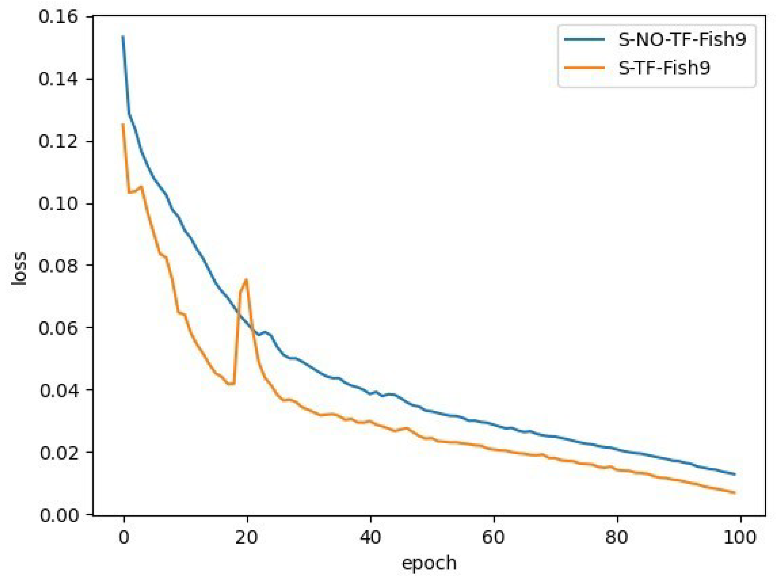
In this section, model S-TF-Fish9 is built on the basis of YOLOv5s using ImageNet pre-trained model initialization, and model S-NO-TF-Fish9 is built using random initialization. Other than that, their model structures, hyperparameters, etc., are unified. The model hyperparameters are set as follows: the training rounds epoch is 100, the batch size is 64, the SGD optimization algorithm is used, the momentum parameter momentum is 0.939, the weight decay is 0.0005. the learning rate is linear decay, the initial value is 0.01, the final value is 0.0001, the preheat warmup epochs are set to 3, the IoU threshold in training is set to 0.2, etc. The parameters in the subsequent subsections are the same.

The training process loss variation is shown in Figure 9.

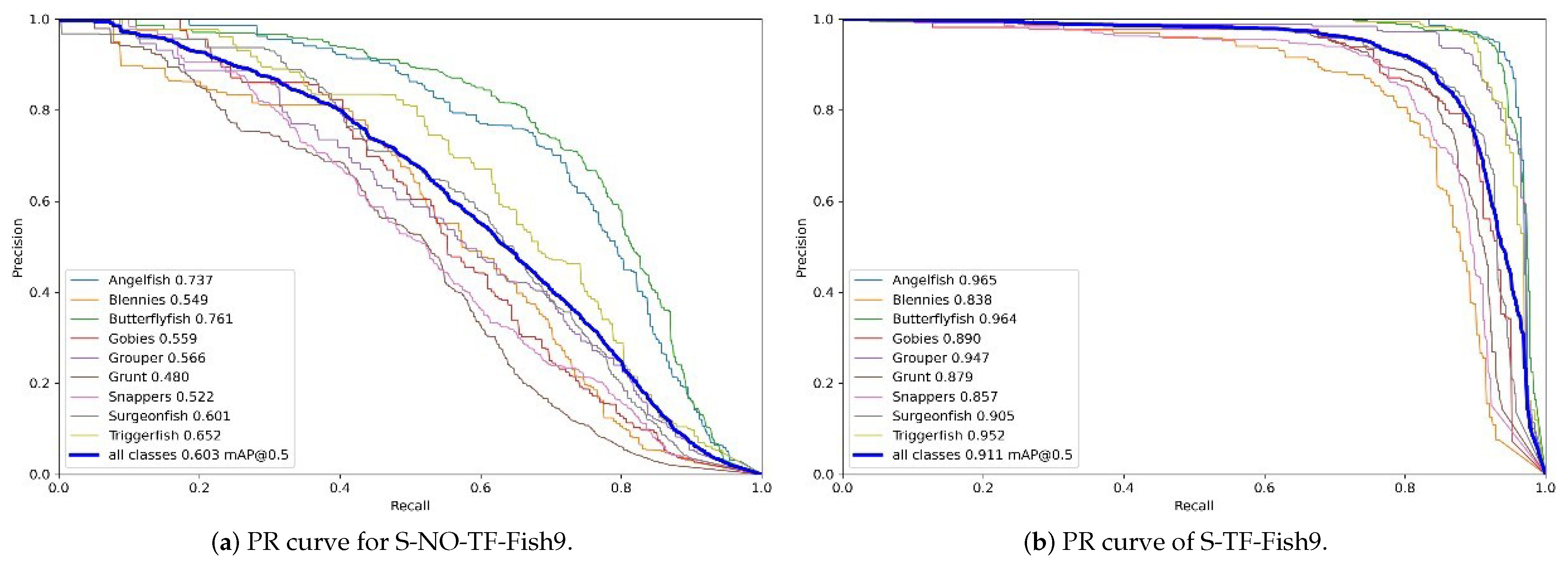
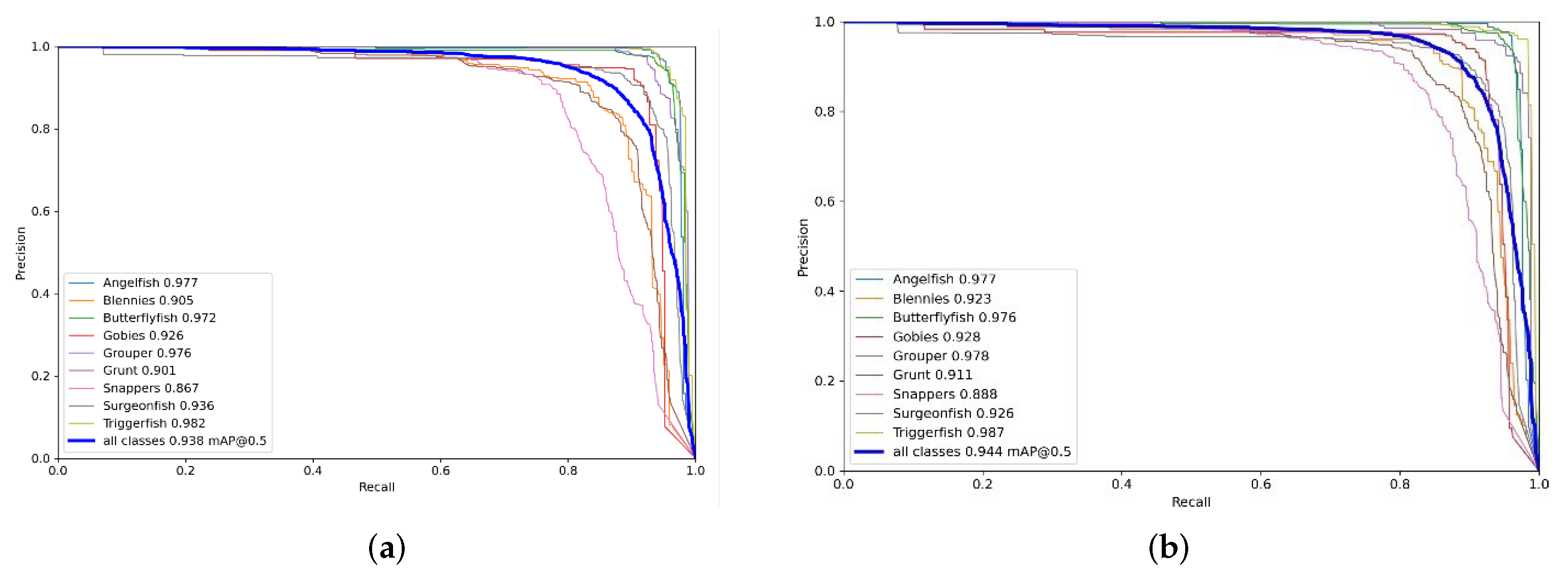
The curve of PR for model S-NO-TF-Fish9 is shown in Figure 10a The curve of PR for model S-TF-Fish9 is shown in Figure 10b. The performance comparison after the introduction of transfer learning is shown in

Table 5. Comparison of migration learning performance.

Model	[email protected]
S-NO-TF-Fish9	0.603
S-TF-Fish9	0.911

.

From the above experiments, it can be found that the performance of the model has been substantially improved after adding transfer learning, and the model also converges faster with smaller loss values. The AP values of each category are greatly improved, and the mAP is improved from 0.603 to 0.911, which is an improvement of about 51%, which shows that the pre-trained model we obtained on ImageNet is able to express the features better, and, even though there is no picture of the fish we detected on ImageNet, the general features of the object can be learned due to the massive data on ImageNet, which help to improve the feature representation of the model. Therefore, subsequent research will all be based on transfer learning.

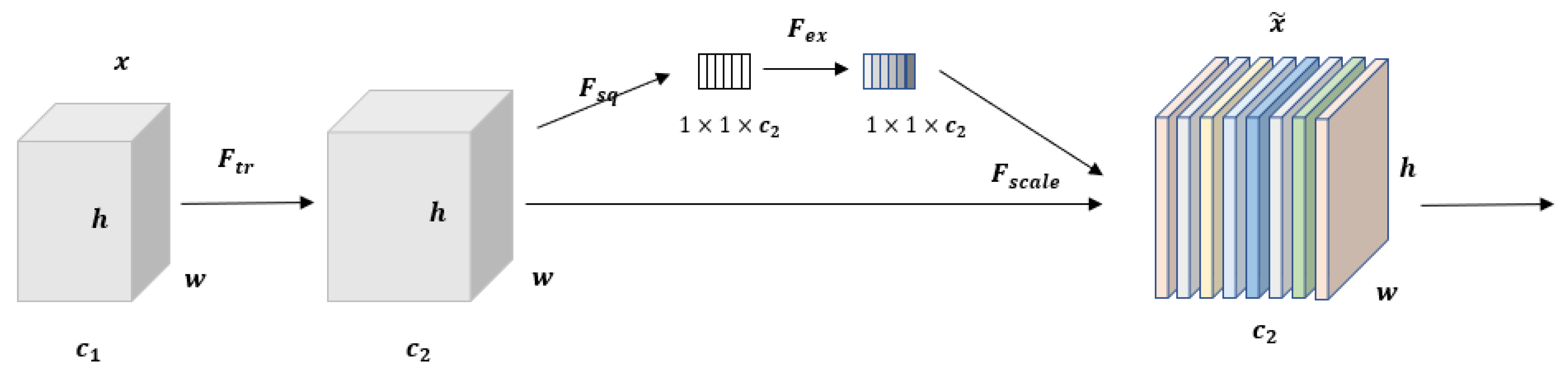
3.4. Attention Mechanisms

In order to strengthen the channel feature expression ability of the model, this paper introduces SENet into the C3 module, and the attention mechanism is introduced into the Backbone end and Head end of YOLOv5s, respectively, to carry out the research. As mentioned in the previous section, YOLOv5s has a total of eight C3 modules, and the Backbone end and Head end each account for four. In order to explore which part of SENet is added to improve the model performance the most, the results of a series of comparison experiments are described in

Table 6. Results of the study on the location of the addition of the attention mechanism.

Distribution Location	[email protected]	Model Size/Mb
Head end all	0.919	13.9
Backbone end all	0.660	14.5
The last two of Head end and Backbone end	0.774	14.5
The first two of Head end	0.916	13.8
The first of Head end	0.926	13.8
The second of Head end	0.900	13.8
The third of Head end	0.912	13.8
The fourth of Head end	0.876	13.8

.

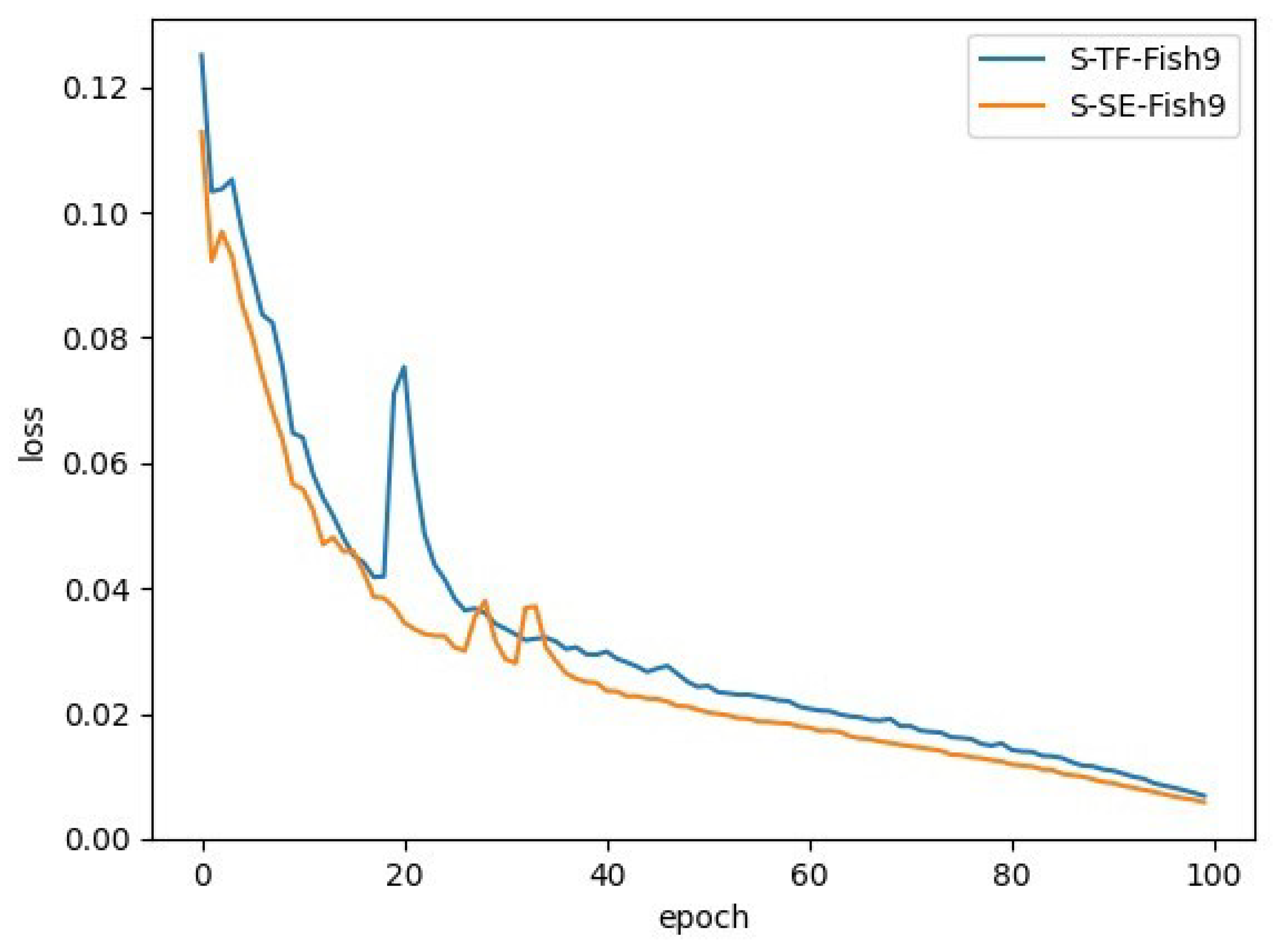
The experimental results show that the introduction of SENet leads to a small increase in the model size. Whether replacing all the C3 modules at the Head end or replacing them at both the Head and Backbone ends, the introduction of SENet at the Head end is optimal. Based on this, and replacing a C3 module individually at the Head end sequentially, the experimental results show that the introduction of SENet at the first C3 module at the Head end is optimal. The model is denoted as S-SE-Fish9, and there is no obvious difference in the size of the different models, and their detection times are almost the same. The variation of the loss curve is shown in Figure 11. The PR curve is shown in Figure 12.

A comparison of the performance of model S-SE-Fish9 and model S-TF-Fish9 is shown in

Table 7. Comparison of attention mechanism performance.

Distribution Location	[email protected]	Model Size/Mb	Detection Time/ms
S-TF-Fish9	0.911	13.7	16
S-SE-Fish9	0.926	13.8	16

.

It can be seen that during training, model S-SE-Fish9 converges faster, has smaller loss values, and has a smoother process of changing losses during training. The mAP of model S-SE-Fish9 is improved by about 1.6%. The time consumed for detecting a single image (size 448 × 640) is the same as the original model; both are 16 ms.

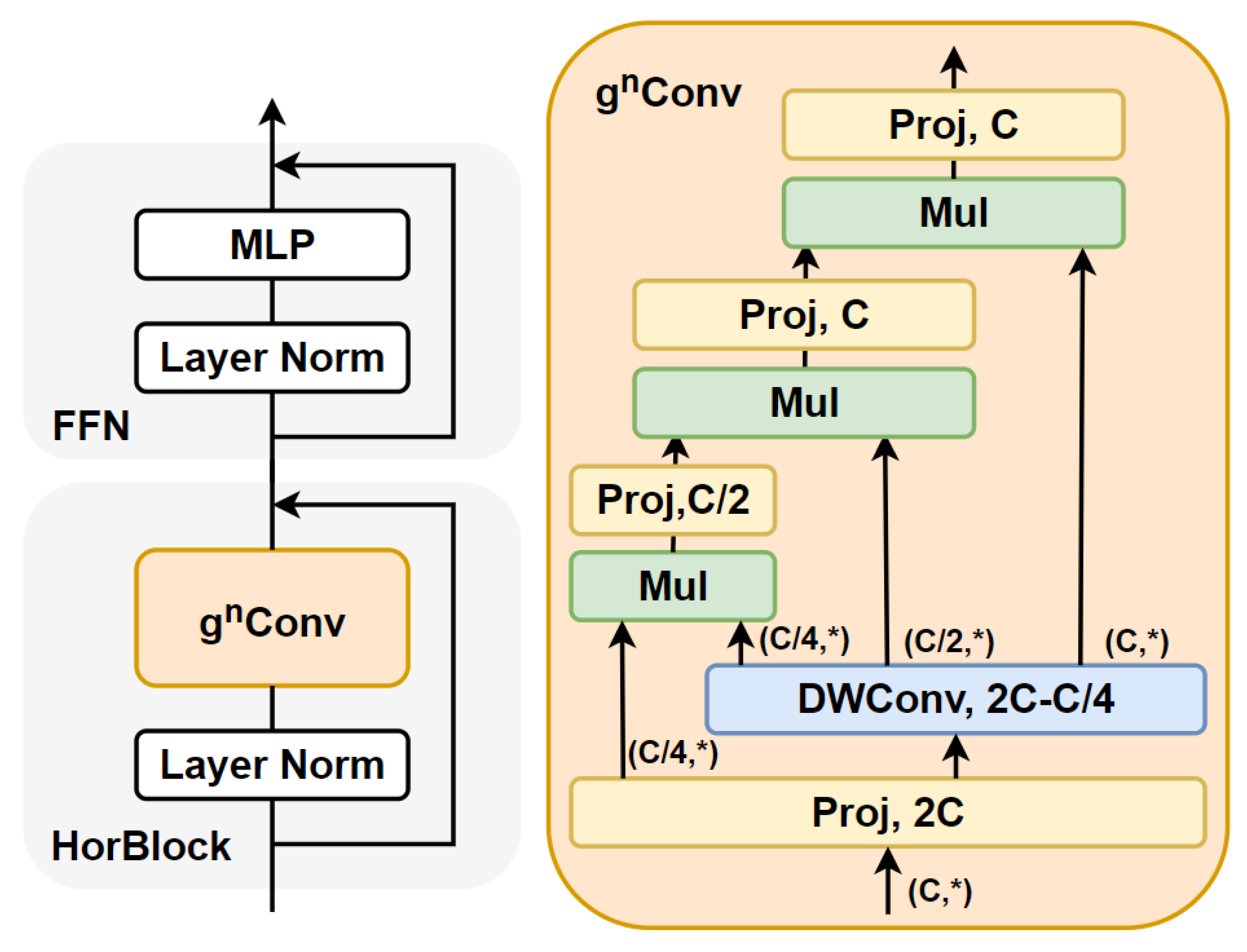
3.5. Gated Convolution

Similarly, in order to verify which place to add HorBlock at the Backbone side is more effective, this paper performs a series of comparative experiments in turn, and the results of the experiments are shown in

Table 8. Results of the study of gated convolutional additive positions.

Distribution Location	[email protected]	Model Size/Mb
Backbone end all	0.883	21.4
The first two of Backbone end	0.900	14.4
The last two of Backbone end	0.929	20.7
The first of Backbone end	0.902	13.8
The second of Backbone end	0.900	14.3
The third of Backbone end	0.880	17.1
The fourth of Backbone end	0.912	17.4

.

The experimental results show that the performance of the model is somewhat improved after the introduction of HorBlock, with the best performance being achieved when added to the last two C3s at the Backbone end, which is notated as S-HorBlock- Fish9. At the same time, it is worth noting that, unlike the attention mechanism module, which brings only a small amount of model size improvement, the gated convolution leads to a large amount of parameter enhancement due to the fact that it will be interacting with the feature layer domain space; it leads to a large number of parameter enhancements, which is visualized as a model size enhancement. 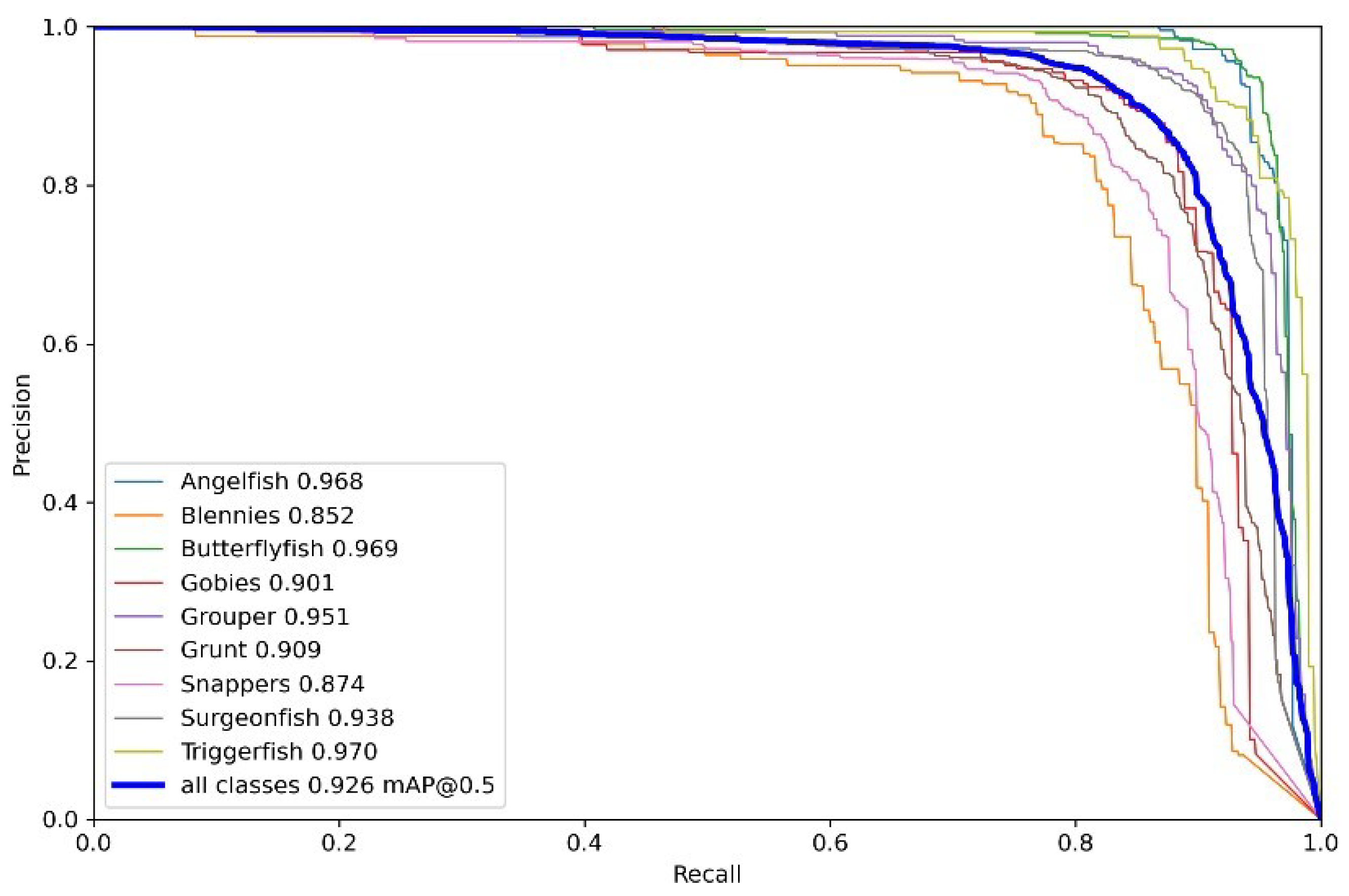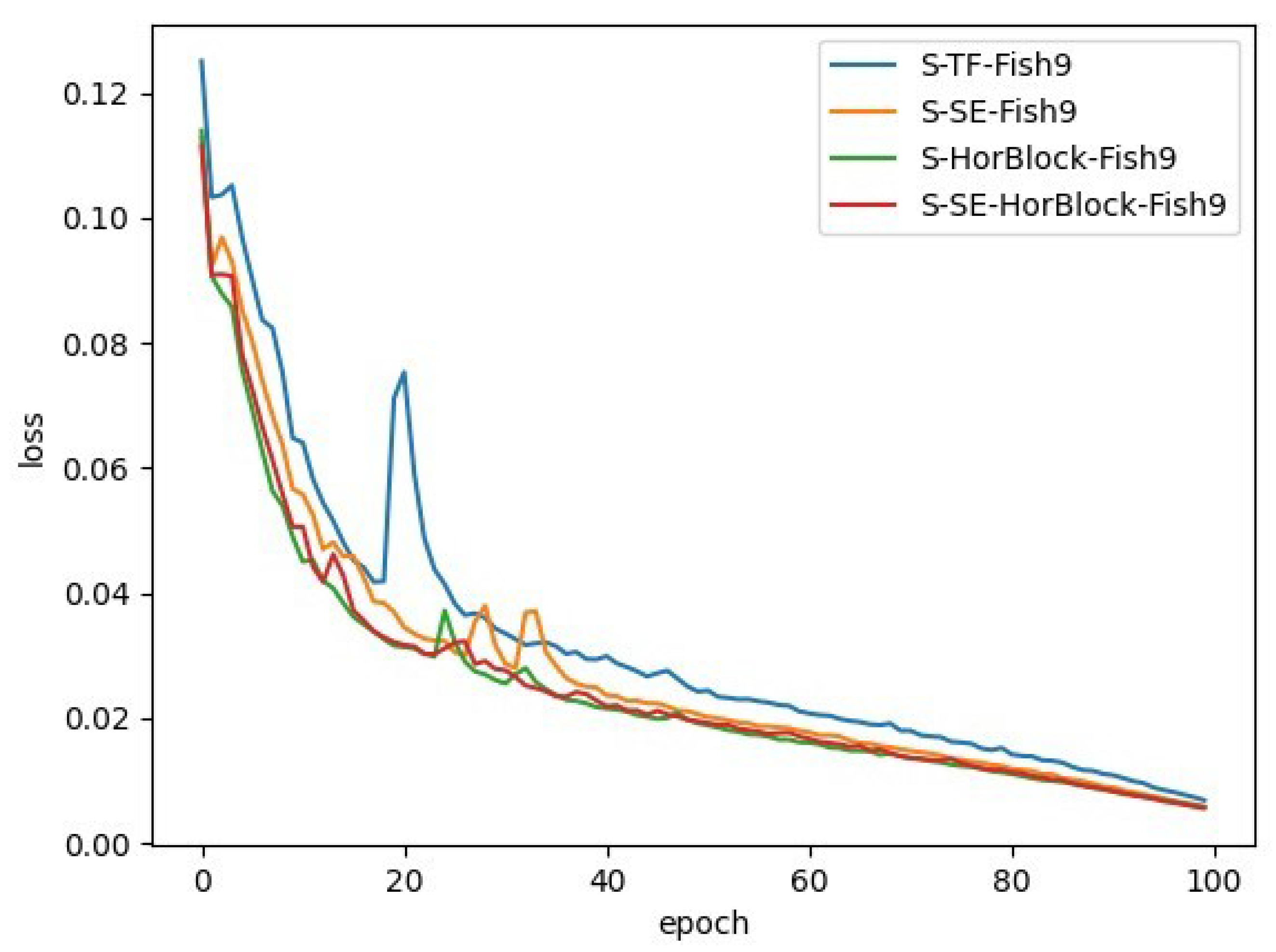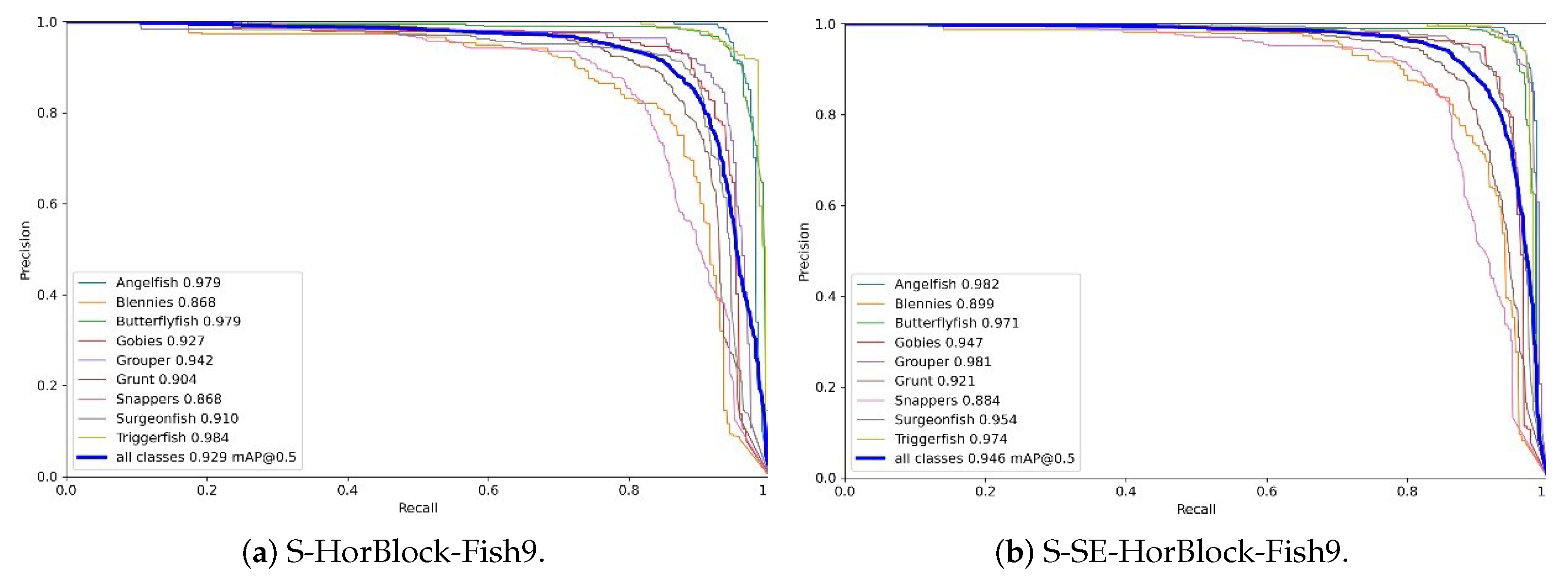In this study, both the gated convolution and the attention mechanism are introduced, where the attention mechanism is introduced in the first C3 part of the Head side as described in Section 3.4. Considering that the gated convolution will lead to a significant increase in the number of parameters (model size) as described earlier, the number of HorBlocks is reduced to one in this study, which is added in the last C3 part of the Backbone side. The model is denoted as S-SE-HorBlock-Fish9. The loss curves and PR curves for model S-HorBlock-Fish9 and model S-SE-HorBlock-Fish9 are shown in Figure 13 and Figure 14.

Compared to the original model, whether introducing the attention mechanism or gated convolution, the model can converge faster, and the training process has less jitter, smoother loss changes, and smaller loss values. When only HorBlock was introduced, the mAP value of the model also increased from the original 0.911 to 0.929; after introducing both SENet and HorBlock, the mAP value of the model increased from the original 0.911 to 0.946. The experimental results for each model are shown in

Table 9. Performance comparison of simultaneous introduction of attention mechanism and gated convolution.

Distribution Location	[email protected]	Model Size/Mb	Detection Time/ms
S-TF-Fish9	0.911	13.7	16
S-SE-Fish9	0.926	13.8	16
S-HorBlock-Fish9	0.929	20.7	19
S-SE-HorBlock-Fish9	0.946	17.4	17

.

From the above table, it can be seen that compared to model S-TF-Fish9, the model size of model S-SE-Fish9 is almost unchanged, and the model detection accuracy is improved by about 1.6%. In addition, the detection accuracy of model S-HorBlock-Fish9 is improved by about 2% but, at the same time, the model size is improved by about 51%. The detection accuracy of model S-SE-HorBlock-Fish9 has been improved the most, by about 3.8%, and the model size has been improved by about 27%. In addition, the detection time of the three models is basically the same.

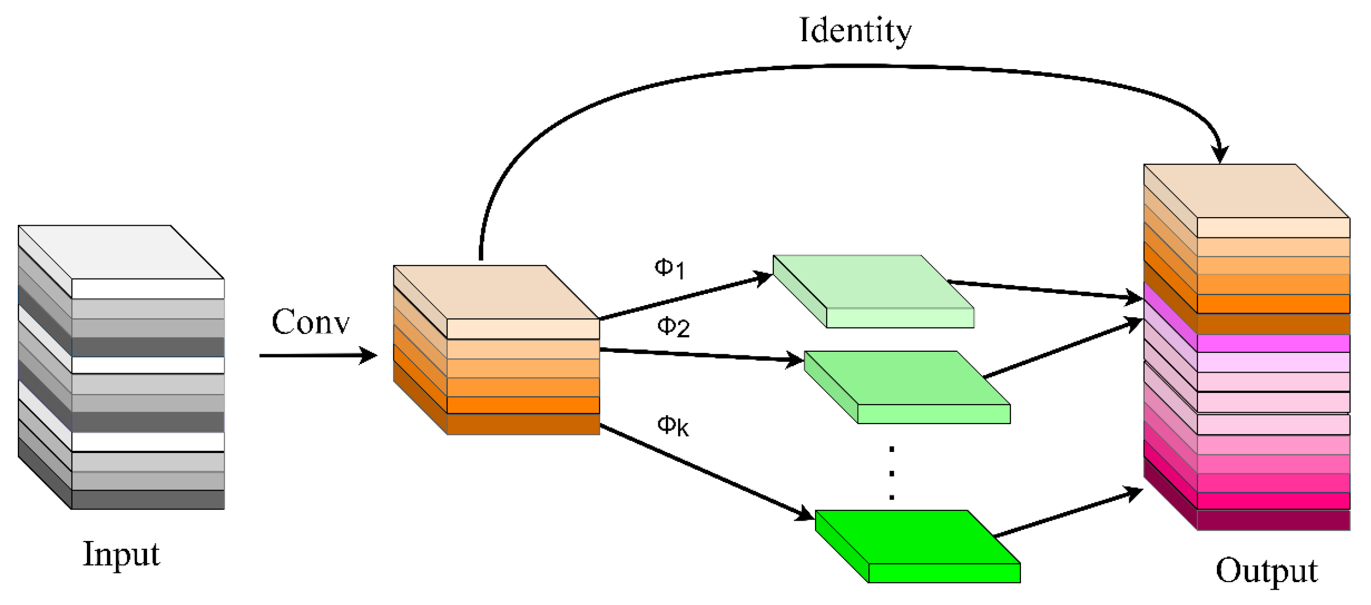
3.6. GhostNet

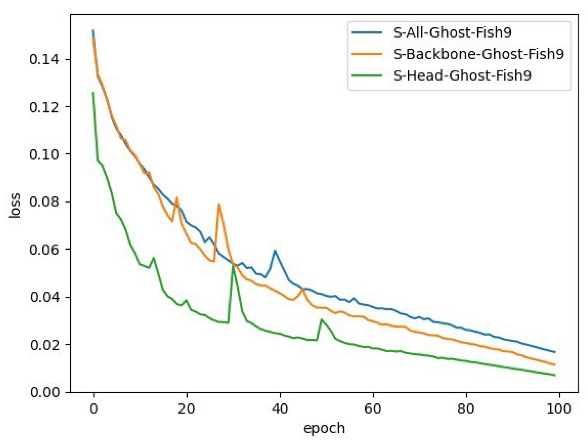
In this study, GhostNet was added to the Head end, Backbone end, and both Head and Backbone ends of YOLOv5s, respectively, to obtain three sets of control models named S-Head-Ghost-Fish9, S-Backbone-Ghost-Fish9, and S-All-Ghost-Fish9. Their loss variations are shown in Figure 15.

The experimental results are shown in

Table 10. GhostNet performance comparison.

Model	[email protected]	Model Size/Mb	Detection Time/ms
S-All-Ghost-Fish9	0.727	7.5	16
S-Backbone-Ghost-Fish9	0.751	10.1	16
S-Head-Ghost-Fish9	0.938	11.1	17

.

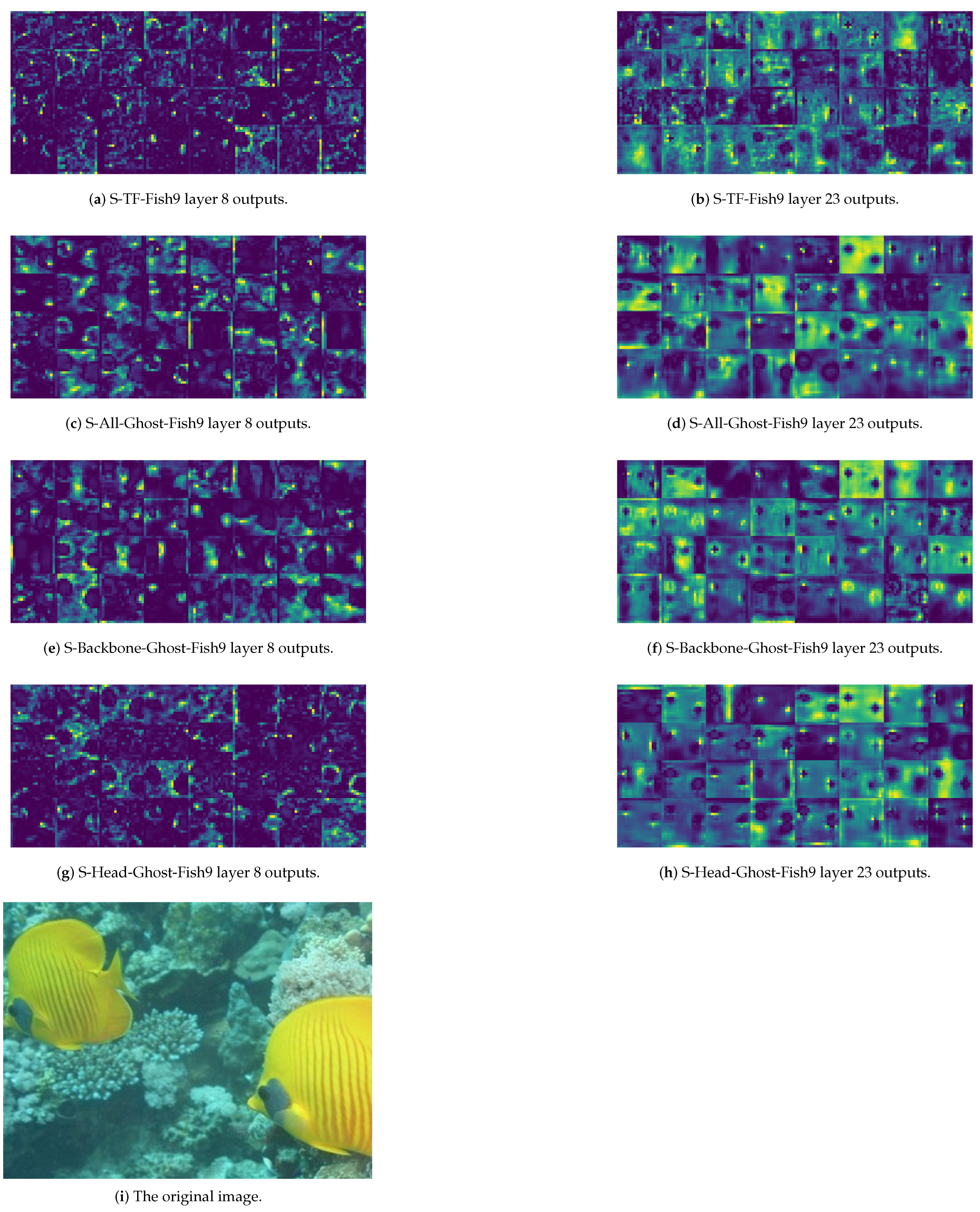
The outputs of the different models are also shown through feature map visualization. Specifically, this study inputs the same image to the models, respectively, and since the last convolutional layers at the Head end and Backbone end are the 8th and 23rd layers, respectively, this study visualizes the outputs of the four models and selects the first 32 of them (four rows and eight columns), as shown in Figure 16.

Comparing Table 10, there is no significant difference in the detection time of the three models, and, according to the mAP values of the different models, it can be found that S-Head-Ghost-Fish9 is more effective, and the mAP is improved by about 24.9% and 29% compared to S-All-Ghost-Fish9 and S-Backbone-Ghost-Fish9, respectively. To summarize, the GhostNet module added to the Head side of YOLOv5 can improve the accuracy of the model, and, at the same time, can have some model pruning effect.

3.7. Improved YOLOv5 Algorithm

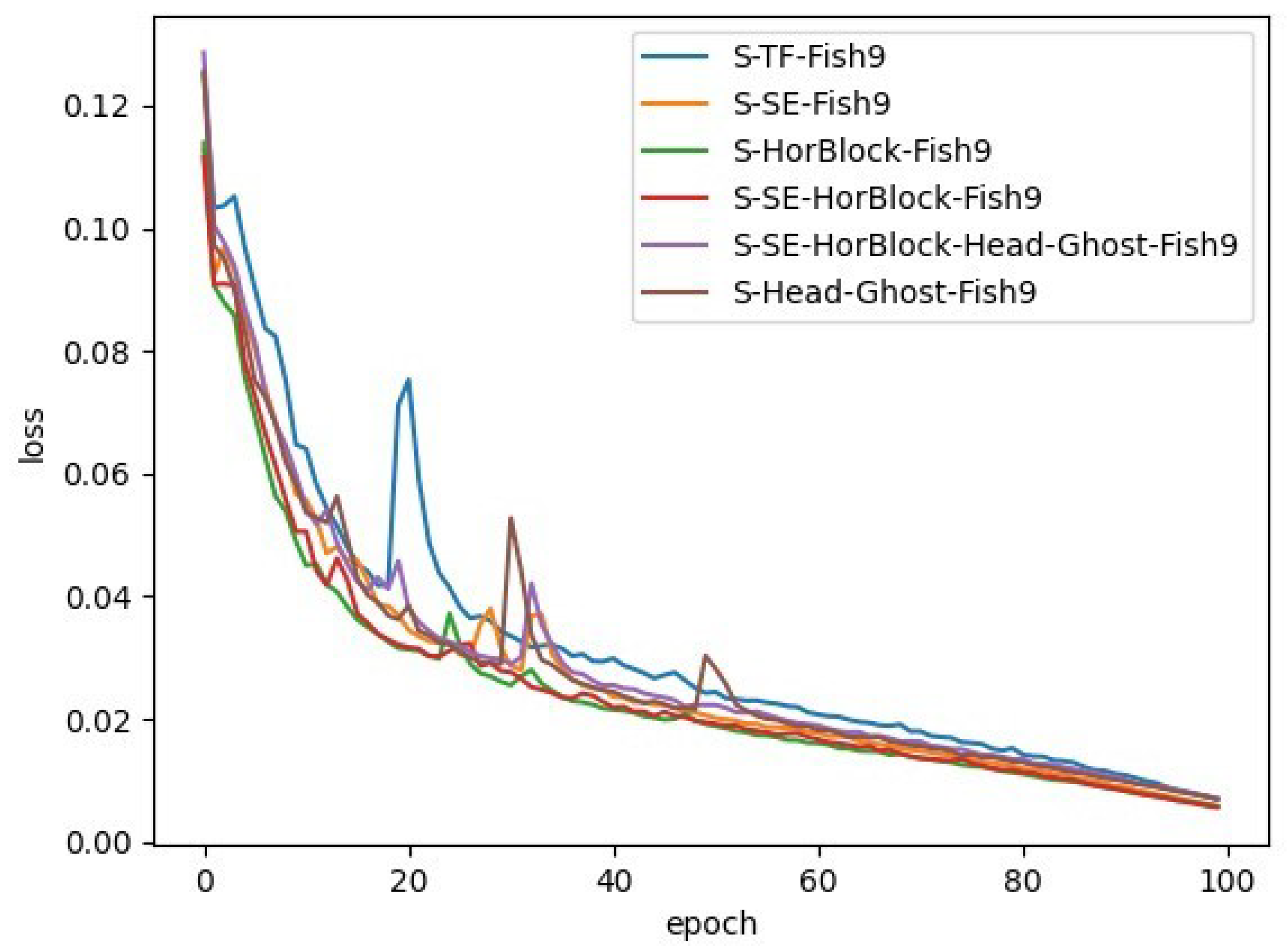
Based on the original YOLOv5s algorithm, through transfer learning research, attention mechanism research, gated convolution research, and GhostNet research, the experiments found that the transfer learning can significantly improve the detection accuracy of the model, and the mAP was improved by about 51% after the introduction of transfer learning. Meanwhile, the attention mechanism can enhance the channel expression ability of the model, and the gated convolution can strengthen the spatial modeling ability of the model; this paper finally determines two improvement schemes: one is to introduce GhostNet in the Head end, which is notated as S-Head-Ghost-Fish9, and the other is to build on the model S-SE-HorBlock-Fish9, and the Head part introduces GhostNet, which is notated as S-SE-HorBlock-Head-Ghost-Fish9. The training loss diagram of each model is shown in Figure 17, and the model performance comparison is shown in

Table 11. Performance comparison of different models.

Model	[email protected]	Model Size/Mb	GFLOPs	Detection Time/ms
S-TF-Fish9	0.911	13.7	15.9	16
S-SE-Fish9	0.926	13.8	15.9	16
S-HorBlock-Fish9	0.929	20.7	22.9	19
S-SE-HorBlock-Fish9	0.946	17.4	17.6	17
S-Head-Ghost-Fish9	0.938	11.1	13.4	17
S-SE-HorBlock-Head-Ghost-Fish9	0.944	15.0	15.4	18
YOLOv6-Fish9	0.935	38.7	45.2	8
YOLOv8-Fish9	0.954	21.4	28.7	16

. The PR curves of the improved models are shown in Figure 18.

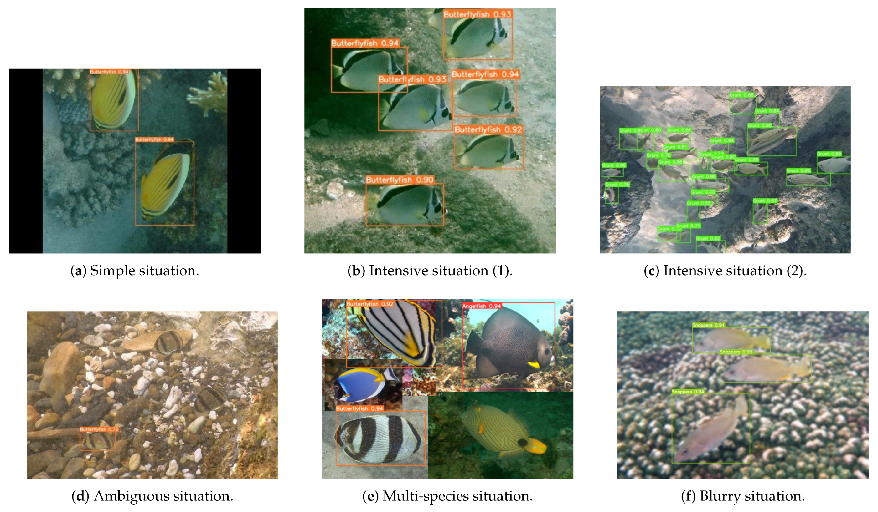
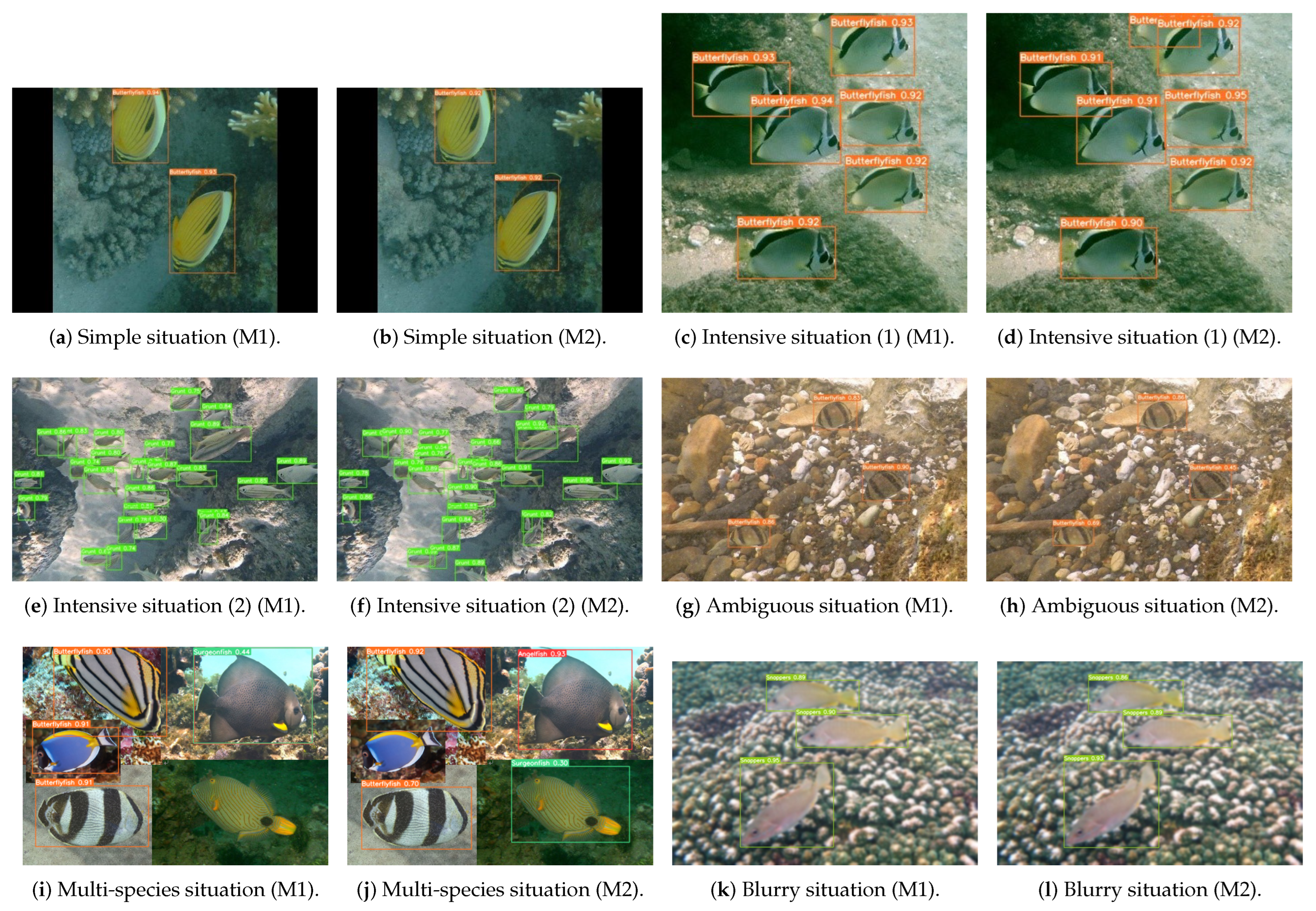
The two improved models were compared to the original model and some of the detection results are shown in Figure 19 and Figure 20.

Figure 18 corresponds to the original model S-TF-Fish9, Figure 19 corresponds to model S-Head-Ghost-Fish9 and model S-SE-HorBlock-Head-Ghost-Fish9. We have compared the performance of the original model and improved models under five different scenarios. Here, since most of the fish in the dataset live together in the same population, it is difficult to include different types of fish in the same image. We concentrated several images together to simulate the situation of different types of fish in the same image. In the simple situation, the improved model localizes the box more accurately and, in the intensive situation, there are fewer missed detections when using improved models. In addition, when the fish body is closer to the background color, the improved models still have better performance. In the multi-species situation, the original model has missed detections while our improved models reduce missed detections. As for the blurry situation, all the models have good detection results. The performance comparisons of the different models are shown in Table 11, in which YOLOv6 is the detection model released by Meituan for industrial applications, which adopts a large number of heavily parameterized modules and is characterized by fast speed, high accuracy, friendly deployment, etc. YOLOv8 is the model released by the YOLOv5 team in early 2023. In this study, the s-size models are used uniformly, and the above two models correspond to YOLOv6-Fish9 and YOLOv8-Fish9, respectively.

In this paper, from the comprehensive consideration of the mAP value, model size, computation amount, and detection time, we found that there was no significant difference in the detection time of each of the improved models, among which three models performed the best; model S-SE-HorBlock-Fish9 had the highest mAP value of 0.946; model S-Head-Ghost-Fish9 had the smallest size and computation amount of 11.1 Mb and 13.4 GFLOPs, respectively. However, model S-SE-HorBlock-Fish9 had a small increase in both size and computation compared to the original model, considering that the current model deployment tends to be lighter, while model S-SE-HorBlock-Head-Ghost-Fish9 had a difference of only 0.02 in mAP. And, the model size and computation are both reduced, so the best models in this study were selected as S-Head-Ghost-Fish9 and model S-SE-HorBlock-Head-Ghost-Fish9.

Relative to the original model, the former improves the mAP by about 3%, reduces the model size by about 19%, and reduces the computation by about 15.7%; the latter improves the mAP by about 3.6%, increases the model size by about 9.5%, and reduces the computation by about 3.1%. Compared to the latest detection models, in which YOLOv6 uses a large number of reparametrized modules, mainly to reduce the hardware latency, which tend to be deployed, the detection time is only 8 ms. YOLOv8, on the other hand, is structurally re-designed with a Decoupled-Head structure, which separates the classification and localization, alleviating the inherent conflicts therein, and the detection accuracy is slightly higher than that of the improved model. The model proposed in this study still has a comparable detection accuracy compared to the latest model, with a slight reduction of about 1%, but has a lower model size, lower model computation, and is more friendly for model deployment.

By introducing the attention mechanism, the representation ability of the model is improved, which allows the network to better focus on useful information. In addition, the gated convolution greatly improved the modeling capability of the model. Through these methods, the mAP of the proposed model is hugely improved. Moreover, the introduction of GhostNet reduces redundancy in the model parameters, so we achieve a lightweight model. Here, the reduction in the model size by the GhostNet module is not obvious; on the one hand, it is due to the fact that the model of YOLOv5s itself is small and the space for model compression is limited, and, on the other hand, after the study in Section 3.6, it is shown that it can still be compressed by 45% in the limiting case. However, from the perspective of the detection accuracy of mAP, the ability of introducing GhostNet at the Backbone side to improve model performance is still debatable. However, from the perspective of model deployment and mAP values, it still makes sense to bring limited model compression while significantly improving detection accuracy. Meanwhile, the above improvement scheme is still relevant to the large models of other versions of YOLOv5 (l and x) and the latest model.

4. Conclusions

In this paper, we first investigated the impact of transfer learning on the model and verified the benefits brought by the pre-trained model, i.e., the ability to accelerate the model convergence while significantly improving the model performance. Then, starting from the model’s channel expression ability and spatial interaction ability, the attention mechanism and gated convolution were introduced, respectively, and compared with the original model; the mAP was improved by 1.6% and 2%, respectively. However, at the same time, gated convolution brought more parameters, which meant the size of the model became larger. Therefore, the model was lightened by introducing GhostNet and added to different places (Head end and Backbone end) of the model, which was evaluated by the mAP value and feature map visualization. The experimental results showed that GhostNet was more effective when added to the Head end of the model. Finally, the decision-making basis of the model was visualized by means of the heat map, and the improved model has a more accurate decision-making range, as well as localization ability.

Through a series of model comparisons, this paper finalized two improved models, S-Head-Ghost-Fish9 and S-SE-HorBlock-Head-Ghost-Fish9, with the former being smaller in model size. In terms of detection speed, a single image took about 17 ms, both of which can meet the demand of real-time detection, and in terms of detection accuracy, compared with the original model, the former was improved by 3% and the latter by 3.6%. Compared with the latest detection algorithms, the above-proposed model has a lower size and computational effort while maintaining a comparable accuracy, which is more conducive to the deployment of the model.

In this paper, by adding improvements to the original YOLOv5s model, we finally achieved the accurate detection of marine fish through our improved lightweight object detection model. Since we used supervised learning to train the object detection model, the improved models could only detect and recognize the nine fish species annotated in our dataset. If we want to achieve the detection of more fish species, we only need to expand our dataset and train the model.

In the future, this proposed method can be applied to seabed removable equipment to obtain the population and number of marine fish and make certain assessments of the marine ecological environment, so as to better realize the protection of marine fish resources.

References

1. Moniruzzaman, M.; Islam, S.M.S.; Bennamoun, M.; Lavery, P. Deep Learning on Underwater Marine Object Detection: A Survey. In Advanced Concepts for Intelligent Vision Systems, Proceedings of the 18th International Conference (ACIVS 2017), Antwerp, Belgium, September 18-21, 2017; Lecture Notes in Computer Science; BlancTalon, J., Penne, R., Philips, W., Popescu, D., Scheunders, P., Eds.; Springer: Cham, Switzerland, 2017; Volume 10617, pp. 150–160. [Google Scholar] [CrossRef]
2. Garcia, G.S.; Dias, M.S.; Longo, G.O. Trade-off between number and length of remote videos for rapid assessments of reef fish assemblages. J. Fish Biol. 2021, 99, 896–904. [Google Scholar] [CrossRef] [PubMed]
3. Hsiao, Y.H.; Chen, C.C.; Lin, S.I.; Lin, F.P. Real-world underwater fish recognition and identification, using sparse representation. Ecol. Informatics 2014, 23, 13–21. [Google Scholar] [CrossRef]
4. Cutter, G.; Stierhoff, K.; Zeng, J. Automated Detection of Rockfish in Unconstrained Underwater Videos Using Haar Cascades and a New Image Dataset: Labeled Fishes in the Wild. In Proceedings of the 2015 IEEE Winter Applications and Computer Vision Workshops, Waikoloa, HI, USA, 6–9 January 2015; pp. 57–62. [Google Scholar] [CrossRef]
5. Ravanbakhsh, M.; Shortis, M.R.; Shafait, F.; Mian, A.; Harvey, E.S.; Seager, J.W. Automated fish detection in underwater images using shape-based level sets. Photogramm. Rec. 2015, 30, 46–62. [Google Scholar] [CrossRef]
6. Aiadi, O.; Khaldi, B.; Saadeddine, C. MDFNet: An unsupervised lightweight network for ear print recognition. J. Ambient. Intell. Humaniz. Comput. 2023, 14, 13773–13786. [Google Scholar] [CrossRef] [PubMed]
7. Khasawneh, N.; Fraiwan, M.; Fraiwan, L. Detection of K-complexes in EEG waveform images using faster R-CNN and deep transfer learning. BMC Med Informatics Decis. Mak. 2022, 22, 297. [Google Scholar] [CrossRef] [PubMed]
8. Li, X.; Shang, M.; Qin, H.; Chen, L. Fast accurate fish detection and recognition of underwater images with Fast R-CNN. In Proceedings of the OCEANS 2015—MTS/IEEE Washington, Washington, DC, USA, 19–22 October 2015; pp. 1–5. [Google Scholar] [CrossRef]
9. Sung, M.; Yu, S.C.; Girdhar, Y. Vision based real-time fish detection using convolutional neural network. In Proceedings of the OCEANS 2017—Aberdeen, Aberdeen, UK, 19–22 June 2017; pp. 1–6. [Google Scholar] [CrossRef]
10. Miyazono, T.; Saitoh, T. Fish Species Recognition Based on CNN Using Annotated Image. In Proceedings of the iCatse International Conference on IT Convergence and Security (ICITCS), Seoul, Republic of Korea, 25–28 September 2017; Lecture Notes in Electrical Engineering. Kim, K., Kim, H., Baek, N., Eds.; Springer: Singapore, 2018; Volume 449, pp. 156–163. [Google Scholar] [CrossRef]
11. Xu, W.; Matzner, S. Underwater Fish Detection Using Deep Learning for Water Power Applications. In Proceedings of the 2018 International Conference on Computational Science and Computational Intelligence (CSCI), Las Vegas, NV, USA, 12–14 December 2018; pp. 313–318. [Google Scholar] [CrossRef]
12. Cai, K.; Miao, X.; Wang, W.; Pang, H.; Liu, Y.; Song, J. A modified YOLOv3 model for fish detection based on MobileNetv1 as backbone. Aquac. Eng. 2020, 91, 102117. [Google Scholar] [CrossRef]
13. Zhao, Z.; Liu, Y.; Sun, X.; Liu, J.; Yang, X.; Zhou, C. Composited FishNet: Fish Detection and Species Recognition From Low-Quality Underwater Videos. IEEE Trans. Image Process. 2021, 30, 4719–4734. [Google Scholar] [CrossRef] [PubMed]
14. Connolly, R.M.; Jinks, I.K.; Shand, A.; Taylor, M.D.; Gaston, T.F.; Becker, A.; Jinks, E.L. Out of the shadows: Automatic fish detection from acoustic cameras. Aquat. Ecol. 2022, 57, 833–844. [Google Scholar] [CrossRef]
15. Underwater Photography—Fish Database. Available online: http://www.fishdb.co.uk/ (accessed on 20 October 2023).
16. Redmon, J.; Divvala, S.; Girshick, R.; Farhadi, A. You Only Look Once: Unified, Real-Time Object Detection. In Proceedings of the 2016 IEEE Conference on Computer Vision and Pattern Recognition (CVPR), Las Vegas, NV, USA, 27–30 June 2016; pp. 779–788. [Google Scholar] [CrossRef]
17. Redmon, J.; Farhadi, A. YOLO9000: Better, Faster, Stronger. In Proceedings of the 2017 IEEE Conference on Computer Vision and Pattern Recognition (CVPR), Honolulu, HI, USA, 21–26 July 2017; pp. 6517–6525. [Google Scholar] [CrossRef]
18. Redmon, J.; Farhadi, A. YOLOv3: An Incremental Improvement. arXiv 2018, arXiv:1804.02767. [Google Scholar]
19. Wang, C.Y.; Bochkovskiy, A.; Liao, H.Y.M. Scaled-YOLOv4: Scaling Cross Stage Partial Network. In Proceedings of the 2021 IEEE/CVF Conference on Computer Vision and Pattern Recognition (CVPR), Nashville, TN, USA, 20–25 June 2021; pp. 13024–13033. [Google Scholar] [CrossRef]
20. Lin, T.Y.; Dollar, P.; Girshick, R.; He, K.; Hariharan, B.; Belongie, S. Feature Pyramid Networks for Object Detection. In Proceedings of the 2017 IEEE Conference on Computer Vision and Pattern Recognition (CVPR), Honolulu, HI, USA, 21–26 July 2017; pp. 936–944. [Google Scholar] [CrossRef]
21. Liu, S.; Qi, L.; Qin, H.; Shi, J.; Jia, J. Path Aggregation Network for Instance Segmentation. In Proceedings of the 2018 IEEE/CVF Conference on Computer Vision and Pattern Recognition, Salt Lake City, UT, USA, 18–23 June 2018; pp. 8759–8768. [Google Scholar] [CrossRef]
22. Hu, J.; Shen, L.; Sun, G. Squeeze-and-Excitation Networks. In Proceedings of the 2018 IEEE/CVF Conference on Computer Vision and Pattern Recognition, Salt Lake City, UT, USA, 18–23 June 2018; pp. 7132–7141. [Google Scholar] [CrossRef]
23. Rao, Y.; Zhao, W.; Tang, Y.; Zhou, J.; Lim, S.N.; Lu, J. HorNet: Efficient High-Order Spatial Interactions with Recursive Gated Convolutions. arXiv 2022, arXiv:2207.14284. [Google Scholar]
24. Han, K.; Wang, Y.; Xu, C.; Guo, J.; Xu, C.; Wu, E.; Tian, Q. GhostNets on Heterogeneous Devices via Cheap Operations. Int. J. Comput. Vis. 2022, 130, 1050–1069. [Google Scholar] [CrossRef]
25. Han, K.; Wang, Y.; Tian, Q.; Guo, J.; Xu, C.; Xu, C. GhostNet: More Features from Cheap Operations. In Proceedings of the 2020 IEEE/CVF Conference on Computer Vision and Pattern Recognition (CVPR), Seattle, WA, USA, 13–19 June 2020; pp. 1577–1586. [Google Scholar] [CrossRef]
26. Pan, S.J.; Yang, Q. A Survey on Transfer Learning. IEEE Trans. Knowl. Data Eng. 2010, 22, 1345–1359. [Google Scholar] [CrossRef]
Figure 1. Fish4knowledge dataset.
Jmse 11 02156 g001
Figure 2. Labeled Fishes in the Wild dataset.
Jmse 11 02156 g002
Figure 3. ImageCLEF dataset.
Jmse 11 02156 g003
Figure 4. Partial image of the Fish9 dataset.
Jmse 11 02156 g004
Figure 5. YOLOv5 structure.
Jmse 11 02156 g005
Figure 6. SENet structure diagram.
Jmse 11 02156 g006
Figure 7. HorBlock Structure.
Jmse 11 02156 g007
Figure 8. GhostNet structure.
Jmse 11 02156 g008
Figure 9. Comparison of migration learning loss.
Jmse 11 02156 g009
Figure 10. Comparison of migration learning PR curves.
Jmse 11 02156 g010
Figure 11. Change in S-SE-Fish9 losses.
Jmse 11 02156 g011
Figure 12. PR curves of S-SE-Fish9.
Jmse 11 02156 g012
Figure 13. Loss curves for S-HorBlock-Fish9 and S-SE-HorBlock-Fish9.
Jmse 11 02156 g013
Figure 14. PR curves for S-HorBlock-Fish9 and S-SE-HorBlock-Fish9.
Jmse 11 02156 g014
Figure 15. Loss profile with the introduction of GhostNet.
Jmse 11 02156 g015
Figure 16. Feature maps of different models.
Jmse 11 02156 g016
Figure 17. Loss curves for different models.
Jmse 11 02156 g017
Figure 18. PR curve of the improved model. (a) PR curves for model S-Head-Ghost-Fish9. (b) PR curves for model S-SE-HorBlock-Head-Ghost-Fish9.
Jmse 11 02156 g018
Figure 19. Original model detection results.
Jmse 11 02156 g019
Figure 20. Improved model detection results. M1 means model S-Head-Ghost-Fish9, M2 means model S-SE-HorBlock-Head-Ghost-Fish9.
Jmse 11 02156 g020