Article

Discrete Element Analysis of Ice-Induced Vibrations of Offshore Wind Turbines in Level Ice

1
Naval Architecture and Ocean Engineering College, Dalian Maritime University, Dalian 116023, China
2
School of Naval Architecture Engineering, Dalian University of Technology, Dalian 116024, China
3
State Key Laboratory of Structural Analysis for Industrial Equipment, Dalian University of Technology, Dalian 116024, China
*
Author to whom correspondence should be addressed.
J. Mar. Sci. Eng. 2023, 11(11), 2153; https://doi.org/10.3390/jmse11112153
Submission received: 19 October 2023 / Revised: 3 November 2023 / Accepted: 7 November 2023 / Published: 11 November 2023
(This article belongs to the Section Ocean Engineering)

Abstract

:
Self-excited vibrations of offshore structures interacting with sea ice, characterized by low frequency and high amplitudes, pose significant hazards to offshore wind turbines (OWTs) in cold seas. This study employs the discrete element method (DEM) with a parallel bonding model to investigate the interaction between sea ice and OWTs. Two bond-failure models are compared, with the results showing that the model considering stiffness softening and fracture energy provides better alignment with field data in the Bohai Sea. The DEM is employed to analyze the ice-induced vibration of OWTs under varying ice velocities, revealing that brittle failure of sea ice occurs at higher ice speeds, leading to random structure vibration. At slower ice speeds, both brittle and ductile sea ice failure modes result in self-excited vibrations. This suggests a strong connection between self-excited vibration and the brittle-ductile failure of sea ice, influenced by the relative speeds between ice and the structure. This study employs the DEM to elucidate the mechanism of self-excited vibrations in OWTs from the perspective of brittle-ductile sea ice failure. The results show that the DEM model accurately describes the brittle-ductile transition in sea ice failure, and that the structural motion aligns well with field measurements.

1. Introduction

Wind power has gained increasing attention worldwide as countries advance their carbon-neutral policies. With the widespread application of offshore wind turbines (OWTs), the vibration problem of structures under the action of sea ice in cold regions has also attracted a lot of attention.

1.1. Ice-Induced Vibrations in OWTs

OWTs play a crucial role in wind power generation. In Europe, the proportion of new installations comprising OWTs reached 23% in 2019, and a growing trend toward their adoption is also evident on other continents [1]. Notably, large offshore wind farms have been established in cold seas, such as the Baltic Sea (16 GW) and the Bohai Sea and northern Yellow Sea of China (900 MW) [2], with prospects for further expansion into Arctic regions, including the Barents Sea and Kara Sea [3,4]. The construction and operation of OWT farms in cold seas necessitate careful consideration of the sea ice parameters due to potential structural safety risks posed by sea ice [5,6]. Similar to lighthouses and offshore oil platforms in these regions, monopiles or multiple piles of OWTs frequently encounter interactions with sea ice at the waterline. This interaction leads to dynamic ice loads on the structure and ice-induced structural vibrations, which are primary threats to OWTs in cold seas [7,8,9]. In the past, there have been incidents such as the partial liquefaction of the sand-filled core of the caisson-type offshore structure Molikpaq due to cyclic ice loading in April 1986 [10]. These events, resulting from cyclic ice loading on offshore structures, have driven research interest in dynamic ice loads and ice-induced vibrations, which can lead to severe fatigue and structural damage [11]. To mitigate the risks associated with excessive ice loads and ice-induced vibrations, which could potentially lead to structural failure, a conical structure known as an isolation cone has been widely deployed at the waterline of monopile OWTs and offshore oil platforms in the Bohai Sea and northern Yellow Sea. However, the deployment of these anti-ice cones comes at a high economic cost during construction and maintenance, and it also increases wave loads during warmer seasons. Therefore, there is a pressing need to uncover the underlying mechanism of ice-induced vibrations in OWTs to develop more cost-effective strategies for mitigating structural safety risks associated with sea ice.
Offshore wind turbines, characterized by their typical flexible, vertically sided structures, inevitably face ice loads and ice-induced vibrations during interactions with level ice. Previous studies have extensively examined ice loads on monopile structures, such as jacket oil platforms and lighthouses, particularly in regions like the Bohai Sea and Baltic Sea. The ice load on cone-shaped structures exhibits cyclic oscillating characteristics due to regular bending failures in sea ice. An ice force spectrum for narrow conical structures was established using multi-year field measurement data from an oil platform in the northern Bohai Sea [12]. Numerical methods were also employed to predict and analyze ice load characteristics on lighthouses in level ice [13]. On the other hand, structural vibration induced by ice loads poses a significant threat to jacket platforms operating in sea ice conditions. ISO19906 [14] categorizes ice-induced vibrations into three types based on full-scale measurements in the Bohai Sea: intermittent crushing at low ice speeds, frequency lock-in (FLI) at intermediate ice speeds, and continuous brittle crushing at high ice speeds (>0.1 m/s) [14]. Early studies attempted to separate the structural response from the ice load, suggesting that the structural response depends on the breaking frequency of the sea ice [15]. However, the interaction between the sea ice and the structure constitutes a coupled system, where the sea ice dynamics, including sea ice failure and movement, play a vital role. Cyclic loading should also consider the relative speed between the structure and the sea ice as the loading speed. Recent studies on ice-induced vibration have aimed to model the ice–structure interaction as a self-excited vibration system [16]. Dynamic models, such as the van der Pol equation, have been employed to study FLI phenomena [17]. The FLI has also been examined using a nonlinear mathematical model with the structure modeled as an Euler–Bernoulli beam [18]. Notably, low ice speeds typically lead to ductile sea ice failure, while high speeds result in brittle sea ice failure [19]. Consequently, the brittle and ductile failures of the sea ice may manifest in different phases of the vibration, generating a sawtooth-shaped ice load history that serves as an external excitation in the governing equation of structural vibration [20]. Moreover, numerical approaches, such as LS-Dyna, have been utilized to simulate ice spallation during ice–structure interactions, modeling the sea ice with hard zone spalls and crushed soft zones to reproduce regular spallation events [21]. Therefore, the dynamics of sea ice have garnered increased attention in the study of ice-induced vibrations.

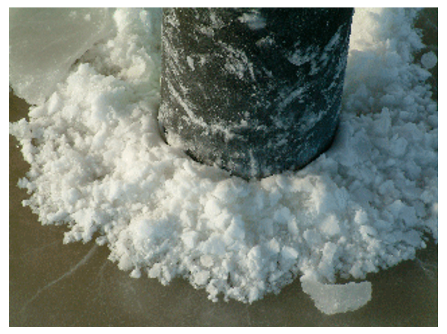
1.2. Failure Mode of Sea Ice

Sea ice possesses a polycrystalline structure at the mesoscale, and its physical and mechanical properties at the macroscale are profoundly influenced by temperature and salinity. As previously mentioned, sea ice exhibits ductile failure at low loading rates and brittle failure at high loading rates, which implies distinct failure strengths under different loading conditions [22]. In the realm of sea ice engineering, the failure modes induced by vertical and conical structures differ, particularly for flexible fixed platforms such as jacket platforms, offshore wind turbines, and lighthouses. Interactions between sea ice and vertical piles tend to result in crushing failure. As the reciprocating motion of the structure involves varying loading rates, the transition between ductile and brittle sea ice failure modes leads to steady-state vibrations of the structure [23]. Of notable concern is the possibility of structural resonance when the ice loading frequency coincides with the structural natural frequency [24]. In the case of interactions between sea ice and wide vertical structures, the ice pressure distribution on the contact surface exhibits a high-pressure zone (HPZ) that decreases from the middle toward both vertical sides. The pressure within the middle of the HPZ can reach several hundred times the average pressure in the contact area [25]. An illustrative example is the Molikpaq, a steel caisson structure with a wide contact area with sea ice. During its deployment in the Canadian Beaufort Sea, the intense ice-induced vibrations of the structure led to the partial liquefaction of the sand-filled core, posing a severe threat to the structural base [10]. Conversely, when sea ice interacts with conical structures, bending failure is the common outcome, and the breaking length becomes a critical factor affecting the ice load [26]. Typically, the frequency of the ice load on conical structures can be much lower than the structural natural frequency, mitigating the risk of structural resonance [11,27]. Therefore, one of the central challenges in the analysis of ice-induced vibrations lies in constructing a mathematical model capable of fully describing the intricate mechanical behavior of sea ice, while also being applicable for engineering-scale analysis. It is difficult to observe the formation mode of internal cracks in sea ice using experimental methods, making it difficult to explain this mechanism. Numerical methods can analyze sea ice failure modes from a microscopic perspective, which can better study structural vibration modes.

1.3. Numerical Methods of Sea Ice

Numerical methods offer a valid approach to model the complex breaking processes of sea ice, with various techniques such as the finite element method, smoothed particle hydrodynamics, and peridynamics having been employed [28]. Among these methods, the discrete element method (DEM) originally designed for simulating granular materials stands out. The DEM tracks the trajectory of individual particles, making it a valuable tool for the detailed analysis of sea ice behavior [29,30,31]. It made its initial foray into sea ice simulations in the 1980s, focusing on aspects like ice floe drift and collision dynamics [32]. Today, the DEM is capable of capturing sea ice deformation, fracture under loading, and fragmentation post-fracture, effectively simulating the entire breaking process [33,34]. In the realm of sea ice dynamics, the DEM has earned a reputation as one of the most effective simulation approaches [35]. DEM simulations of sea ice utilize different geometric elements, including spheres, disks, and polyhedra [36,37,38]. Sphere-based DEM, in particular, offers advantages in contact detection and ease of implementation, making it suitable for large-scale parallel computation using graphics processing units (GPUs) [39]. Typically, spherical elements are bonded to form a continuous ice sheet, with bonds capable of failing under external loads, employing specific bond-failure models. The parallel bonding model (PBM) is one of the most frequently used models for simulating brittle materials, including sea ice and rock. The calibration and application of sphere-based DEM with the PBM in sea ice engineering have advanced rapidly [40,41]. Additionally, several bond-failure criteria have been considered in the DEM simulations of brittle materials, such as criteria accounting for bilinear/trilinear stress-strain relationships, stiffness softening, hybrid fracture energy models, and more [42,43]. Notably, the failure criterion incorporating stiffness softening and hybrid fracture energy can effectively mitigate the instantaneous release of energy, resulting in more stable simulations of brittle material breaking processes [44,45]. These advancements point to potential directions for further research on bond-failure criteria in the DEM simulations of sea ice.
This study introduces a bond-failure model considering the stiffness softening and the hybrid fracture energy in the sphere-based DEM. The interactions between the sea ice and monopile OWT are simulated with the proposed DEM, where the monopile OWT is simplified as a single pile with 3 degrees of freedom (DOF). The field measurement of the oil platform in the Bohai Sea is employed to validate the numerical method. Then, the ice speed effect is studied to analyze different types of ice-induced vibrations of OWT. The innovation of this article lies in analyzing the failure mode and ductile-brittle transition characteristics of sea ice from a microscopic perspective. By explaining the interaction between wind turbine structural vibration and sea ice damage, this article reveals the mechanism of self-excited vibration of the structure.

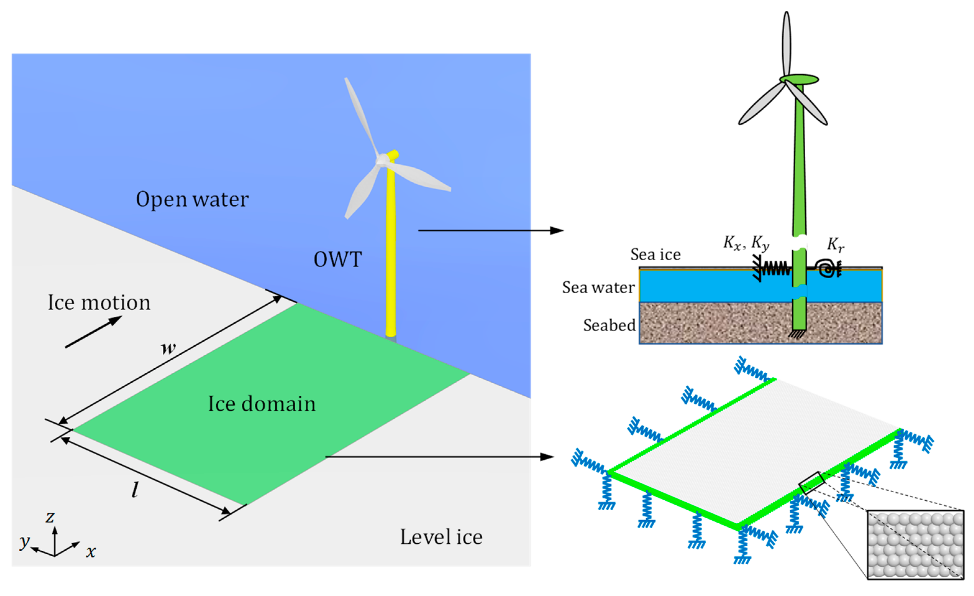
2. Methodology of Sphere-Based DEM for Sea Ice Simulation

Within the sphere-based DEM, the parallel bonding model plays a pivotal role in connecting adjacent sphere elements to create a representation of the continuous ice sheet. To assess bond failures, two traction-deformation models are employed. The first model resembles the traditional unilinear approach, akin to the one originally proposed in the study that introduced the PBM. This approach establishes bonds between adjacent elements based on beam theory and subsequently breaks them using tensile and shear strengths [46]. In contrast, the second model follows the same bonding approach but incorporates a hybrid fracture energy model to govern bond failures. This approach provides an alternative method for modeling bond failure in sphere-based DEM simulations.

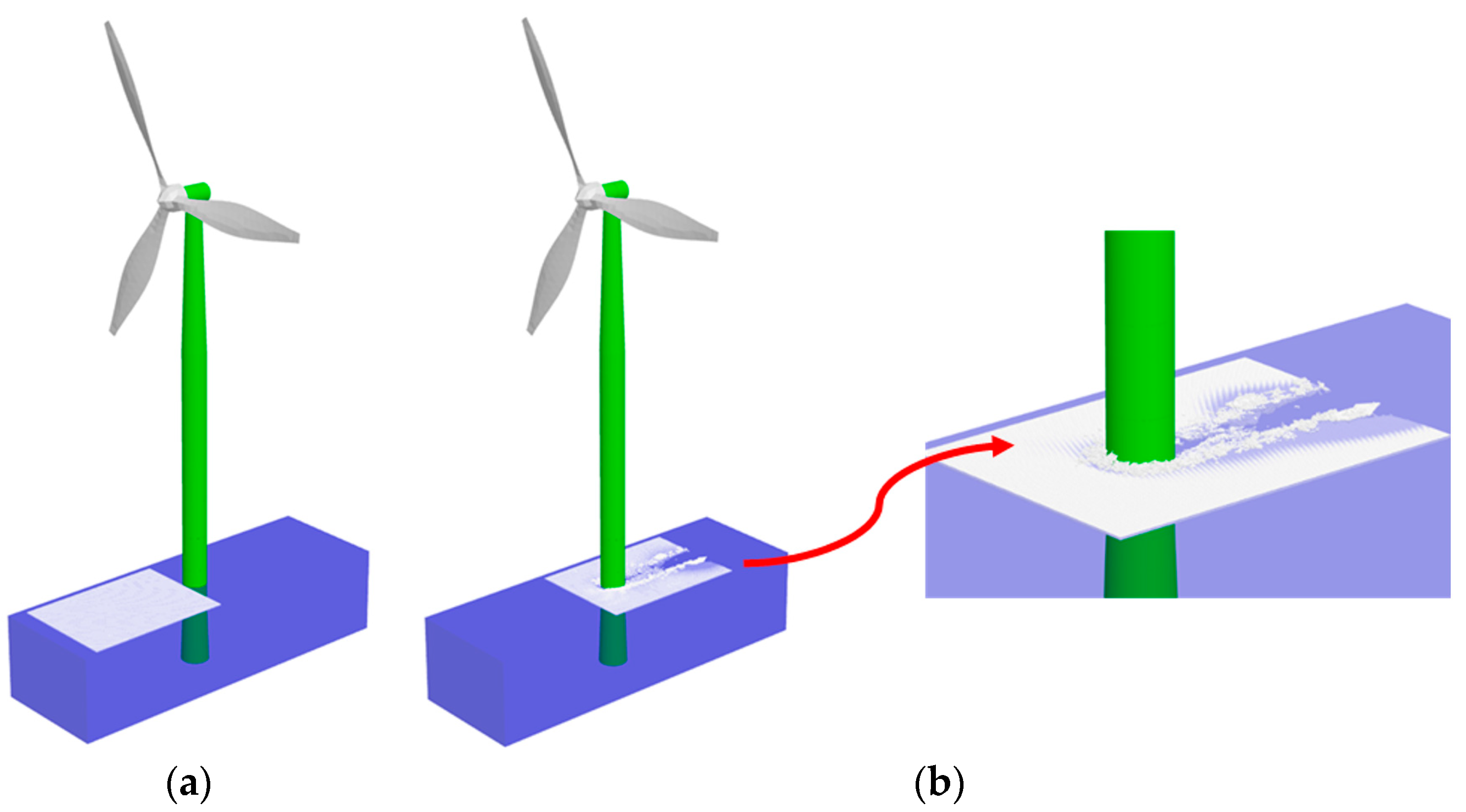
2.1. Model Description of Ice–Structure Interaction in DEM

Sea ice is represented as a collection of equal-sized spheres organized in a hexagonal close packing (HCP) lattice structure [47]. Notably, the HCP lattice structure introduces anisotropic elasticity, in contrast to the statistical isotropic elasticity resulting from random packing. This lattice-structured model effectively reproduces the cracking and fragmentation observed in brittle materials, albeit differing from traditional continuous models. Moreover, the HCP lattice structure provides a framework for establishing a consistent and predictable mechanical behavior, offering a unique local–global parametric relationship. This relationship allows the determination of particle-scale parameters based on given macroscopic elastic parameters such as strength, stiffness, and failure patterns specific to the material. Previous studies have successfully applied the HCP lattice with spherical elements to simulate sea ice fractures during interactions with structures [48,49]. It is worth noting that the local–global parametric relationship within the HCP-structured model is influenced by the size of the spheres [50]. Strength determination is achieved through formula fitting between strengths and sphere size, derived from compressive and bending tests on sea ice in the Bohai Sea [51]. This approach is then validated by comparing simulated ice loads on monopiles with field measurements in the Bohai Sea and model tests at the Hamburg Ship Model Basin [36]. Consequently, employing the HCP arrangement within sphere-based DEM proves to be a valid and effective method for simulating sea ice failure.
In this study, the level ice is assumed to extend infinitely in the horizontal plane. However, directly representing this infinite ice domain within the DEM simulation presents challenges. To address this, a boundary condition incorporating springs, dampers, and constant velocity is employed. As illustrated in Figure 1, three sides of the rectangular ice domain, namely y+, y−, and x−, feature multiple layers of spherical elements. These boundary elements are subject to various constraints to emulate the behavior of an infinite ice domain. To account for the constant motion imparted by the current, these elements are velocity-constrained, with the assumption that the current direction aligns with the x− direction. Consequently, the velocity in the x− direction of the boundary elements matches the current speed. Additionally, the boundary elements are equipped with spring and damper constraints, with stiffness and damping coefficients set to values consistent with those used for spherical elements in the bond force model. By constraining the z direction motion of the boundary elements, the ice model composed of spherical elements can be initialized at a level where gravitational and buoyant forces are balanced. This boundary condition approach effectively addresses the challenge of representing an infinite ice domain within the DEM simulation.
In the DEM simulation, the monopile offshore wind turbine (OWT) is anchored to the seabed, remaining fixed in position. The simulation models only the portion of the structure interacting with the sea ice, as the DEM is not suitable for simulating flexible bodies. This approach is also driven by the fact that the section of the structure near the waterline is the primary region of interest for ice-induced vibration. To model ice-induced vibrations analytically and numerically, a single-degree-of-freedom oscillator is employed, consistent with prior research [16,17]. However, this study extends the model to consider rotational motion within the horizontal plane, encompassing three degrees of freedom: translational motion in the x and y directions and rotational motion along the z-axis. This approach allows for a more comprehensive representation of ice-induced vibrations and their effects on the structure.
Contact detection is a pivotal step in implementing simulations of sea ice failure and the interactions between the structure and the sea ice. Typically, contact detection involves three main phases: neighbor search utilizing a world grid, bounding box detection, and pinpointing contact points [52]. The initial two phases are collectively known as the broad phase search. It is worth noting that contact detection tends to be the most time-consuming aspect of the DEM simulations, particularly when dealing with irregularly shaped elements. In some cases, contact detection can account for a significant portion of the total computation time, often ranging from 70% to 90% [52,53,54]. For spherical elements, contact detection is less complex since the primary geometric feature is the radius. Therefore, the broad phase search is the predominant challenge for spherical elements. In this study, a 3-dimensional grid-based broad phase search algorithm is employed. Conversely, when detecting contact between spherical elements and the monopile, the process is abstracted as a minimum distance solver between a point and a cylinder, with the monopile near the waterline being regarded as a cylinder. Consequently, contact detection in the DEM simulations of this study encompasses detection between spheres and between spheres and a cylinder. Importantly, both types of contact detection can be resolved using analytical solutions, enhancing the efficiency and accuracy of the simulations.

2.2. Governing Equations

The translational and rotational motions of each spherical element are written as follows:
m s d u s d t = F c + F b + F h + F p I s d ω s d t = M c + M b + M h + M p
where m s and I s are the mass and rotational inertia of the sphere, I s = 0.4 m R 2 ; u s and ω s are the translational and rotational velocities, respectively; t is the time; F c is the contact force from all adjacent elements, F b is the bond force from all bonded elements, M c and M b are the torques caused by F c and F b , respectively; F h is the summation of the buoyancy and drag force from the water, M h is the drag moment from the water; F p and M p are the contact force and moment from the pile. The contact and bond force will be introduced in the following sections. The buoyancy of a sphere can be calculated with its immersed volume entirely or partly submerged under the waterline. The drag force, F d , and drag moment, M d , can be calculated with the following formulas [55]:
F d = 1 2 C d F ρ w A s u b u s u w u u w M d = 1 2 C d M r 2 ρ w A s u b ω s ω s
where C d F and C d M are the drag coefficients corresponding to F d and M d , respectively; ρ w is the density of seawater; A s u b is the area immersed in the water; r is the sphere radius; u w is the current speed.
The structural motion considers three degrees of freedom, translational motion in the x and y directions, and the rotational motion in the z direction. The governing equations are as follows:
m p x ¨ + c x ˙ + k x + F x p = 0 m p y ¨ + c y ˙ + k y + F y p = 0 I z θ ¨ z + c θ ˙ z + k θ z + M z p = 0
where m p is the mass of the cylindric pile, and I z is the rotational inertia along the z-axis.
The motion equation is solved explicitly by using the Verlet integral scheme, including the translational displacement (position) and speed, and the rotational speed [56]. The rotational angle is not solved explicitly because it is not required in calculating the contact force, while the bond force demands the increment of the rotational angle only. The time step is determined as [57]
t = γ π r 0.163 ν + 0.877 ρ G
where γ is a constant scalar, normally γ = 0.1 ; r is the radius of the spherical element, ν is the Poisson’s ratio, ρ is the material density, G is the shear modulus, G = E / ( 2 ( 1 + ν ) ) where E and ν are the elastic modulus and Poisson’s ratio, respectively.

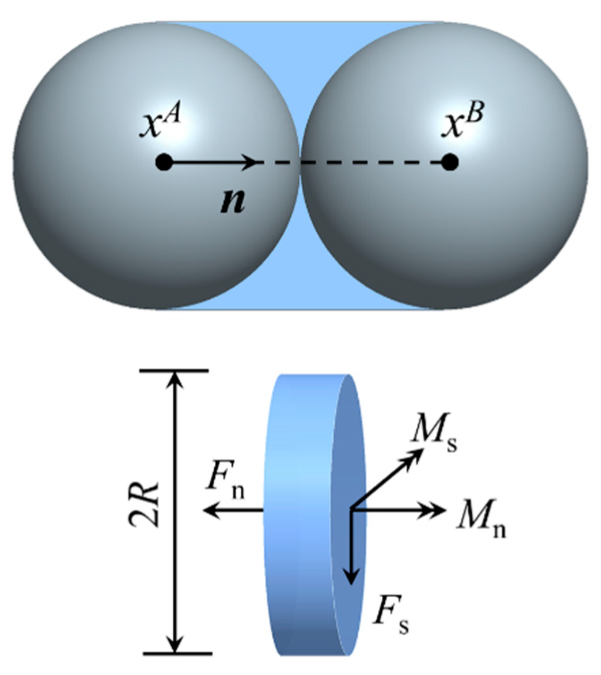
2.3. Contact Force Model of Spherical Elements

The contact force between spherical elements considers the elastic and viscous forces in the normal and shear directions. A linear contact force model is used in this study. The normal contact force, F n c , considering the elastic and viscous components ( F n c e and F n c v , respectively) can be written as
F n c = F n c e + F n c v = K n δ n C n δ ˙ n
where K n is the normal stiffness between two adjacent elements, δ n is the normal overlap of the contact, C n is the normal damping coefficient, and δ ˙ n is the normal relative velocity between two contact points belonging to two elements. The stiffness, K n , can be written as
K n = π E R i R j R i + R j
where E is the elastic modulus of the sea ice, R is the radius of the spherical element, and i and j denote two adjacent spherical elements. The damping coefficient, C n , can be expressed as follows:
C n = ξ n 2 m i j K n
where m i j is the equivalent mass, m i j = m i m j / ( m i + m j ) ; ξ n is the dimensionless damping coefficient, ξ n = ln e / π 2 + ln 2 e , where e is the restitution coefficient.
The shear contact force, F s c , satisfies the Coulomb friction law:
F s c = m i n K s δ s t C s δ ˙ s t ˙ , μ F n
where K s is the shear stiffness between two adjacent elements; C s is the shear damping coefficient; t and t ˙ are the unit vectors of the shear contact overlap and relative shear velocity, respectively; δ s is the shear contact overlap, which is obtained according to the relative tangential velocity and integral step-by-step; δ ˙ s is the relative velocity between two contact points belonging to two elements; and μ is the friction coefficient. K s and C s are proportional to K n and C n with constant parameters α and β , respectively, as follows:
K s = α K n ,   C s = β C n
The two parameters α and β are both equal to 0.1 according to Long et al. [36].
The contact force, F c , and moment, M c , caused by the shear contact force between adjacent elements can be written as follows:
F c = F n c n + F s c s M c = R n × F s c s
where n is the unit normal vector of the contact; s is the unit vector in the shear direction, s = n o r m ( K s δ s t C s δ ˙ s t ˙ ) .

2.4. Parallel Bonding Model of Spherical Elements

In the DEM simulation, the sea ice is represented as an assembly of regularly arranged spherical elements, following a hexagonal packing pattern. The bonding between adjacent spherical elements is established using the parallel bonding model, as proposed by Potyondy and Cundall [46].
The bonding model operates on the premise of a bonding disc, featuring a radius, R, and centered on the contact point within the adjacent region of two elements. This bonding disc serves as a conduit through which bonding forces and moments are concurrently transmitted between the elements, as illustrated in Figure 2. The core principle of the parallel bonding model involves conceptualizing an array of linear springs with consistent normal and tangential stiffness. These springs are centered at the contact point between the two units and are uniformly distributed across the bonded disc. Consequently, the bonding disc effectively facilitates the transfer of bonding forces and moments. In line with the beam theory model, the maximum tensile and shear stresses experienced by the bonded disc can be mathematically expressed as follows:
σ m a x = F n A + M s I R τ m a x = F s A + M n J R
where F n and F s are the normal force and tangential force, respectively; M n and M s are the normal moment and tangential moment, respectively; R is the radius of the disc; A is the area of the disc, J is the polar moment of inertia of the disk, I is the moment of inertia of the disk, expressed as
A = π R 2 , I = 1 4 π R 4 , J = 1 2 π R 4

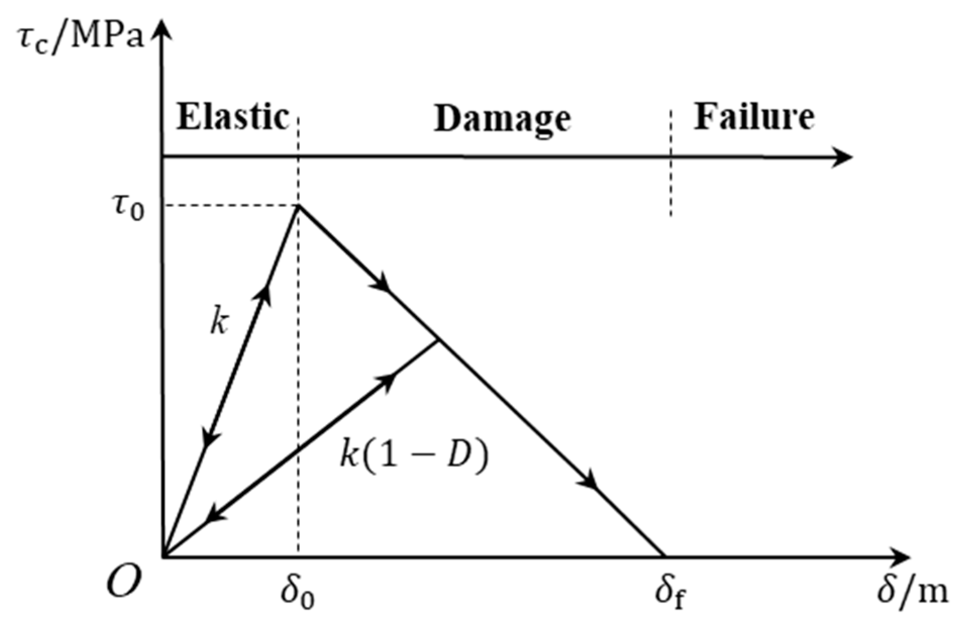
2.5. Bond-Failure Models

(1)
Mohr–Coulomb criterion-based bond-failure model
The tensile and shear strengths, σ t and τ s , satisfy the Mohr–Coulomb criterion, written as [58]
τ s = σ t + μ b σ m a x
where μ b is the internal friction coefficient, and μ b = t a n φ and φ is the angle of internal friction. When the maximum tensile stress and shear stress of the bonded disk exceeds the critical strengths, i.e., σ m a x > σ t and τ m a x > τ s , the bonded disk fails. Thus, the process of the sea ice breakage can be simulated. The Mohr–Coulomb criterion-based bond-failure model is already reported in publications. The size effect of this model has also been studied to determine the relationship between the simulation parameters and the mechanical parameters of the target material. Here, the relationship of the bonding strengths and the mechanical strengths for the sea ice simulation is used [51].
(2)
Hybrid fracture energy-based bond-failure model
The bond-failure model employed in this simulation adopts a linear softening model to characterize the failure process. This choice enables the gradual dissipation of energy generated during the bond-failure process, preventing its instantaneous release and the associated element splashing, particularly when fast energy release occurs. The failure process is divided into three distinct stages, as illustrated in Figure 3: the elastic stage, damage stage, and failure stage. The stiffness of the bonding disc (k) changes during these three stages. To ascertain the elastic stage, the model relies on the comparison of maximum normal and tangential stresses with the strengths. These stages together provide a comprehensive framework for understanding the progression of bond failure in the simulation. The condition that elastic stage ends and damage starts is written as [43]
σ m a x σ t 2 + τ m a x τ s 2 1
The equivalent stress, τ ¯ , and the equivalent deformation, δ ¯ , is calculated by the normal and tangential deformation δ n and δ s , expressed as
τ ¯ = σ m a x 2 + τ m a x 2 δ ¯ = δ n 2 + δ s 2
If Equation (10) is satisfied, the equivalent stress and the equivalent deformation at this point is recorded as τ 0 and δ 0 . The damage coefficient, D , can be calculated as
D = δ f δ 0 δ ¯ δ 0 δ f δ ¯
where δ f is the deformation when the failure occurs.
The damage, D , affects the stiffness of the bonding disc. The stiffness of the bonding disc should be weaker if D increases. Thus, when the bonding disc is in the damage stage, the normal and shear stiffnesses of the bonding disc, K n 0 and K s 0 , are calculated as
K n 0 = K n ( 1 D ) ,   K s 0 = K s ( 1 D )
where K n and K s are the normal and shear stiffnesses in the elastic stage, respectively. On the other hand, the hybrid critical fracture energy, G c , is defined based on the Benzeggagh–Kenane model [59,60].
G c = G I c + ( G I I c G I c ) G I I G I + G I I η
where G I c and G I I c are the fracture energies in the tensile and shear mode, respectively; η is equal to 1.75 for brittle materials [61], and G I I / G I = δ s 2 / δ n 2 . Then, δ f can be determined as δ f = 2 G c / τ 0 . The bond disc will fail if δ ¯ > δ f .
The damage in the bond-failure model used in this study is reflected by the linear softening model, while the hybrid fracture means that the failure criterion considers both normal and tangential forces and deformation to determine the bonding and failure between elements. This approach is different from the determination of the bonding and failure in normal and shear directions separately in Mohr–Coulomb criterion-based bond-failure model introduced above. Moreover, the hybrid fracture energy-based bond-failure model can increase the stability of the simulation in which sea ice compression occurs and many elements are in crushing failure, because the fracture energy is dissipated gradually.

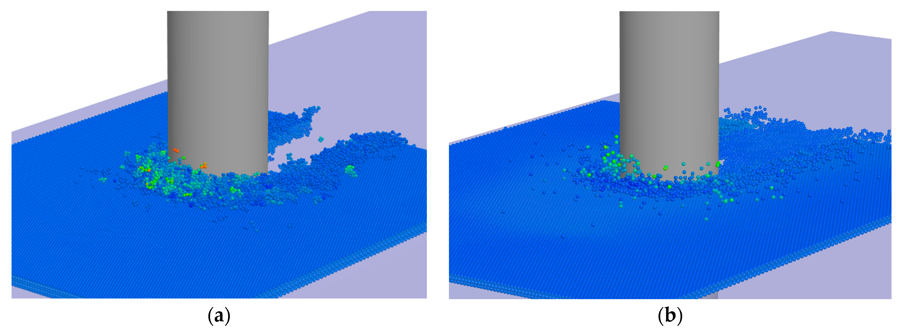
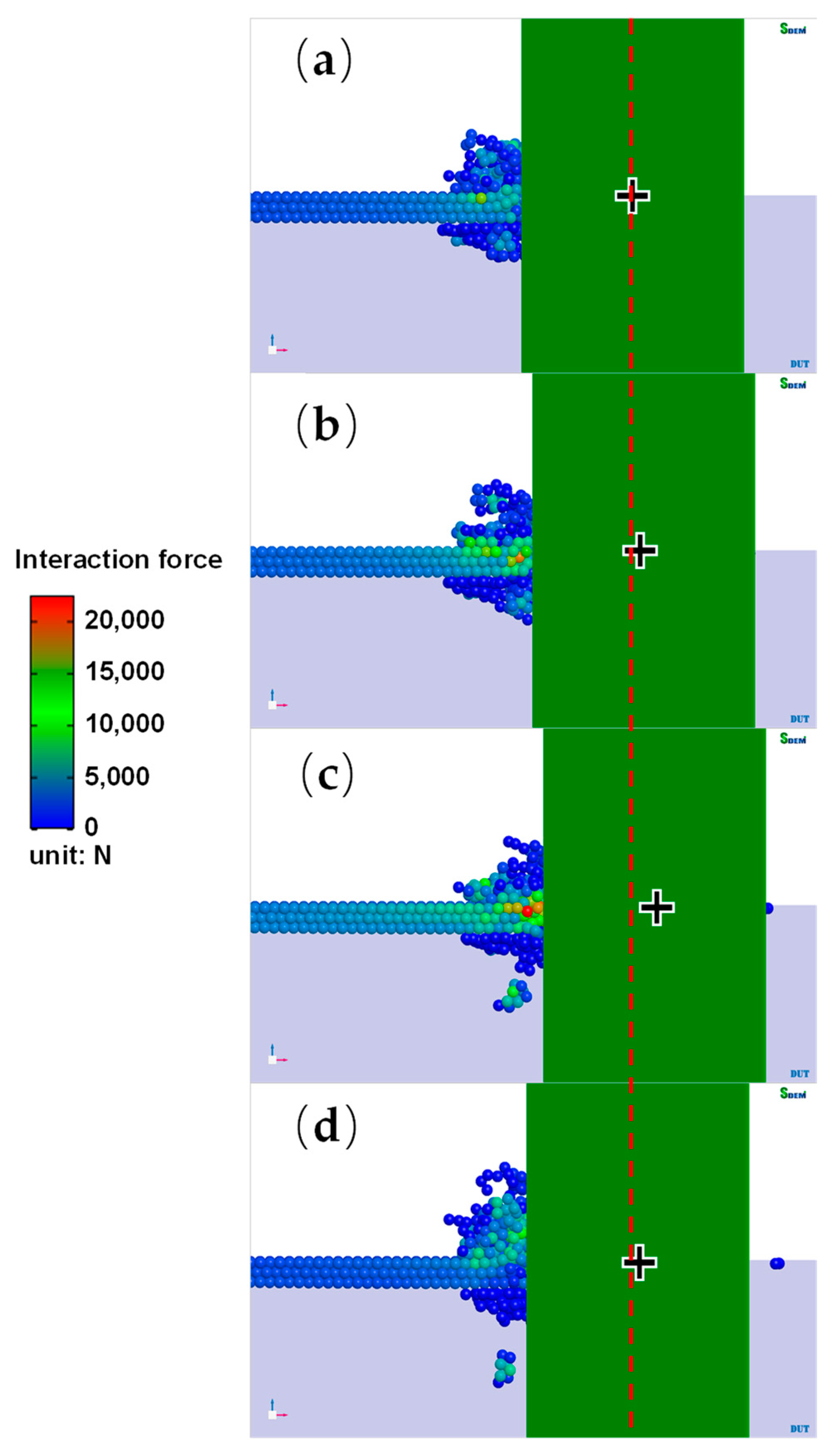
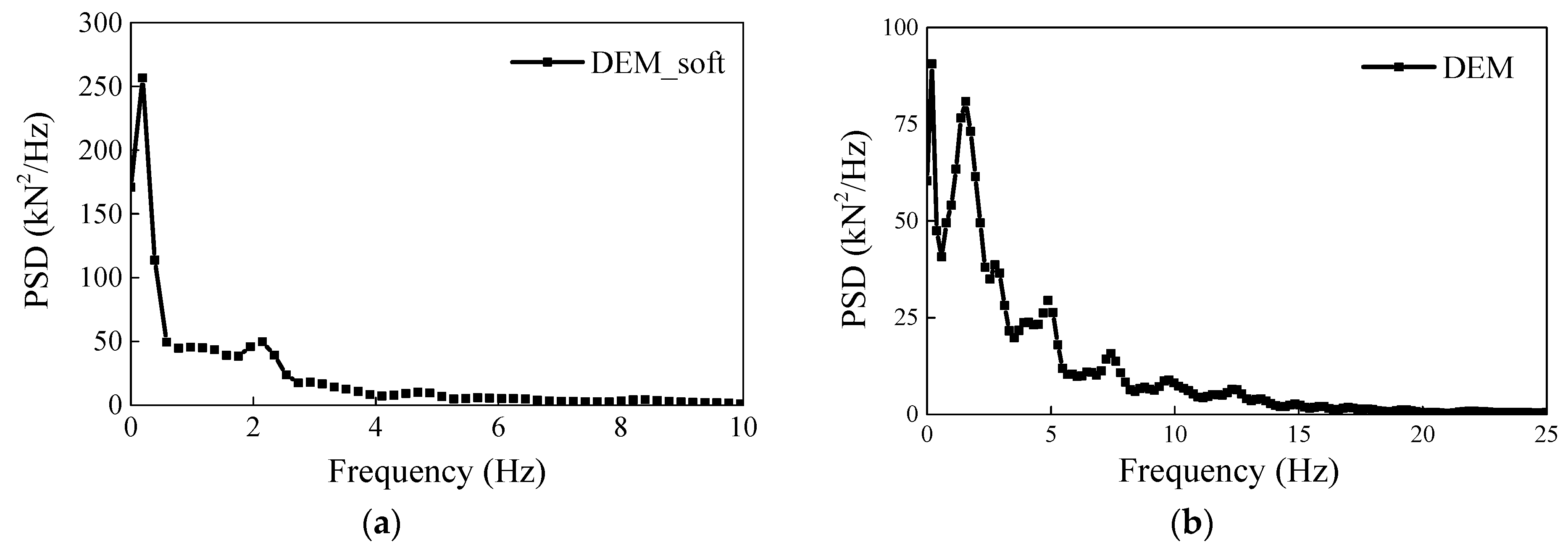
3. Ice Loads on Cylindric Pile Simulated with Different Bond-Failure Models

The algorithm for the DEM simulation is implemented by in-house C++ code and CUDA parallel computing techniques. The neighboring list is built first to detect the adjacent element. The contact force and bond force will be calculated if two adjacent elements are detected. Then, the motion of each element will be solved by the Verlet integral scheme. Thus, new positions are obtained and new neighbors will be generated. The dynamics of the sea ice can then be simulated.
To verify the accuracy of the bond-failure model proposed in this article, two models with or without considering damage were compared to simulate the crush failure of the sea ice during the interaction between the sea ice and the vertical structures. By comparing with the calculation results of the data measured in the Bohai Sea, the differences can be found between the two bond-failure models in simulating the breaking of the sea ice.
The discrete element model has been developed to study the interaction between the sea ice and the vertical pile legs. The model is based on the real dimensions of the JZ9-3MDP vertical pile leg structure in the Bohai region, and it incorporates measured data related to the sea ice. In the simulation, regularly arranged and bonded spherical elements are used to represent the sea ice. The model includes three boundaries where the sea ice does not contact with the structure, and these boundaries are characterized by spring boundaries with fixed stiffness and motion velocity. The chosen sea ice thickness aligns with actual ice conditions in the Bohai Sea, measuring 0.18 m. The actual sea ice size is much larger than the structural size, so the simulated sea ice size should be set as large as possible to offset the impact of size effects [36]. Furthermore, the sea ice velocity is set at 0.2 m/s, and the sea ice strength is specified as 2.3 MPa. For further clarity, the specific discrete element parameters are detailed in Table 1.
Figure 4 illustrates the interaction process between the sea ice and the vertical structures observed in the Bohai Sea. The fractured sea ice depicted in the image takes on a powdered form, consistently being squeezed out of the contact surface. When the ice velocity is high, the sea ice consistently interacts with the structure, resulting in sustained ice loading. Figure 5 showcases simulations of the crushing process between sea ice and vertical structures using two distinct bond-failure models. The simulation outcomes reveal that under both bond-failure models, the sea ice undergoes crushing failure, giving rise to small fragments. This observation aligns with the measurements obtained in the Bohai Sea. However, disparities emerge in how the two bond-failure models simulate the process of sea ice fragmentation. In the bond-failure model considering the softening process, a stiffness softening stage precedes bond failure, with some elements impacting on the structure without undergoing bond failure. These interconnected units can aggregate to form smaller sea ice fragments scattered in proximity to the structure. Conversely, in the tensile-shear fracture criterion model, bond failure occurs as soon as the element contacts the structure, and the scattered elements move at higher speeds without forming a stable accumulation effect. In line with field measurements of sea ice compression, the front end of the ice sheet is pulverized into powder and adheres to each other after interaction with the structure, accompanied by a limited number of fragments. This observation indicates that the mixed fracture criterion, which considers damage, is more aligned with the measured results in the Bohai Sea, and better suited for describing the failure mode of the sea ice.
As a consequence of the brittle crushing failure of the sea ice, the ice load curve following collision with the structure consistently maintains a high frequency and remains greater than 20.0 kN, as depicted in Figure 6. The ongoing fragmentation of the sea ice ensures its continuous contact with the structure, resulting in the persistence of ice loading. This form of ice loading poses a significant threat to the structure. Figure 7 presents a comparison of calculation results using two distinct fracture criteria. When contrasted with Figure 6, it becomes evident that the ice load simulated using the mixed fracture criterion exhibits more continuity and concentration, closely resembling the measured data from the Bohai Sea. This difference arises because the mixed fracture criterion considers the gradual consumption of energy generated during the brittle crushing process of the unit, making energy changes within the unit system more stable. In contrast, when employing the tensile-shear zoning fracture criterion, the instantaneous release of fracture energy due to unit compression causes the unit to splash and rapidly detach from the contact surface between the sea ice and the structure. Furthermore, the influence of unit size results in gaps between the sea ice and the structure upon contact, making it challenging for the ice load to maintain a continuous and stable state. Moreover, when examining the peak and average values of the ice load time history curve, the results of the discrete element simulation using the mixed fracture criterion are notably closer to the measured data from the Bohai Sea.
Spectral analysis is presently the primary method for scrutinizing the random vibration of structures under environmental load excitation. Qu et al. [27] conducted a power spectral density (PSD) analysis on the sea ice crushing load time history data obtained from field experiments. They derived a general form of continuous crushing ice force spectrum characteristics. To delve deeper into the analysis of ice load characteristics on vertical structures, the improved periodic Welch method (pwelch) is employed by MATLAB software (ver. 2009a) to perform self-power spectral density analysis. This analysis encompassed both the ice load data obtained from actual measurements in the Bohai Sea and discrete element simulations. In Figure 8, the self-power spectral density curve of the measured ice load in the Bohai Sea reveals that the power spectral energy predominantly resides in the low-frequency region, diminishing as frequency increases. Notably, no significant peak emerges in the self-power spectral density near the structural vibration frequency, suggesting that the sea ice experiences continuous brittle compression and fragmentation at higher ice speeds, unaffected by random structural vibrations. Figure 9 presents a comparative analysis of the ice force spectrum for discrete element simulations of ice loads under different fracture criteria. When evaluating the ice force spectrum, it becomes evident that the tensile-shear fracture criterion manifests multiple peaks in the low-frequency stage, a deviation from the characteristics of brittle compression fracture observed in the sea ice. In contrast, the ice force spectrum under the mixed fracture criterion aligns more closely with the measured data in the Bohai Sea.
To sum up, the hybrid fracture energy-based failure criterion, which takes into account damage, not only closely aligns with the measured data in ice load values during simulations of sea ice crushing but also accurately represents the brittle crushing failure characteristics of the sea ice in the ice load power spectrum analysis. Therefore, it is better suited for the calculation and analysis of the interaction between sea ice and wind turbine structures.

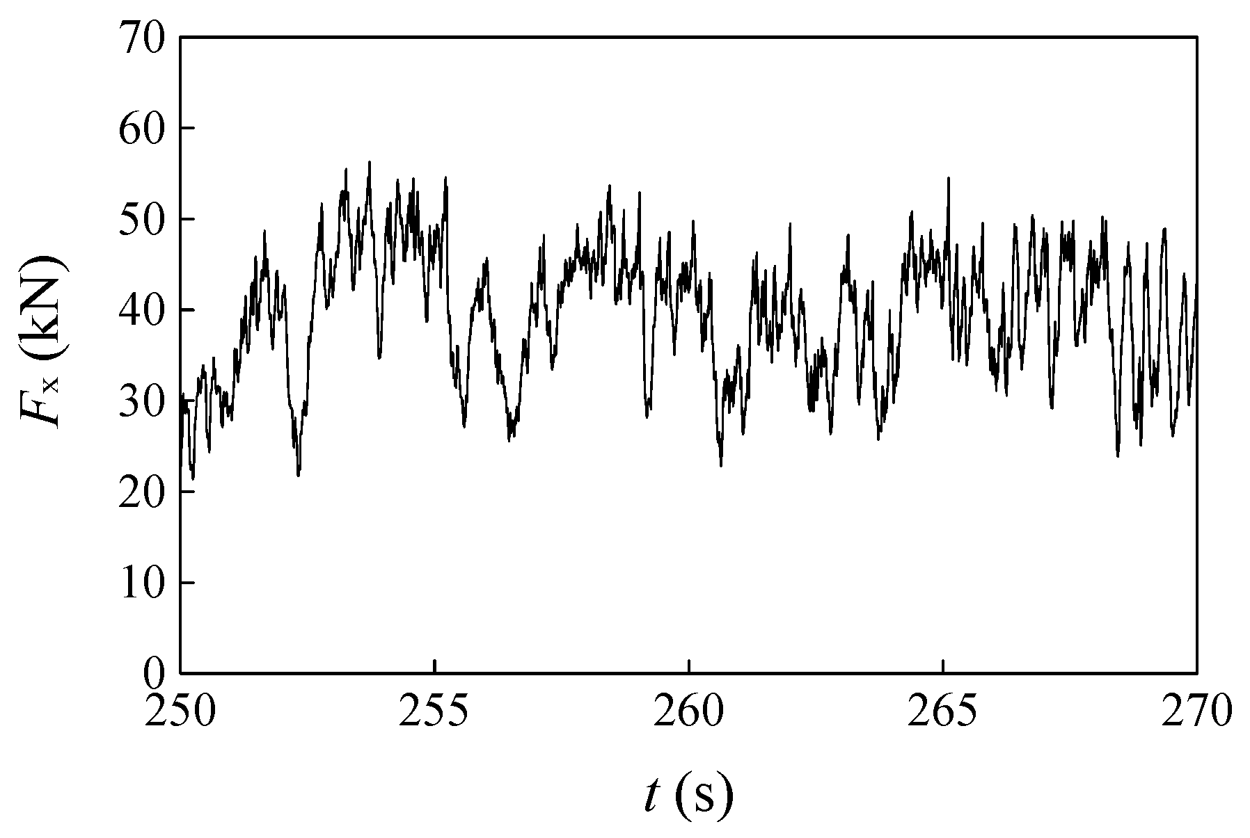
4. Ice-Induced Vibration of Offshore Wind Turbine

Given the expanding utilization of offshore wind turbine structures in cold regions, the occurrence of ice-induced vibration during their interaction with sea ice has garnered significant interest. To investigate the various types, underlying principles, and influencing factors related to self-excited vibration in wind turbine structures, the discrete element method provides a valuable means of assessing the impact of ice velocity on both the ice load and ice-induced vibrations experienced by these structures.

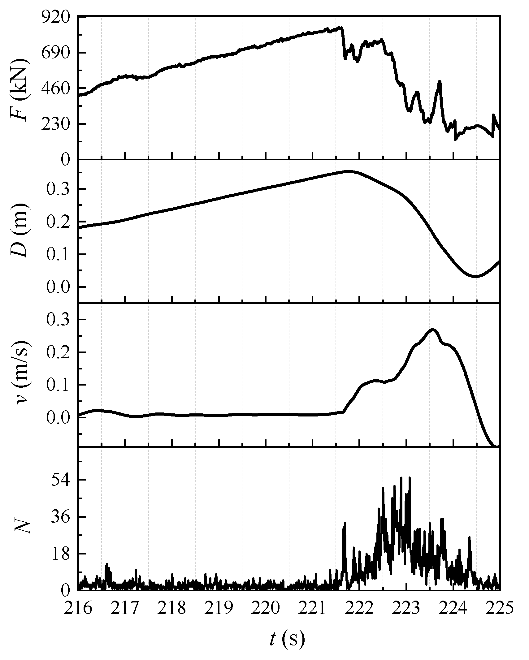
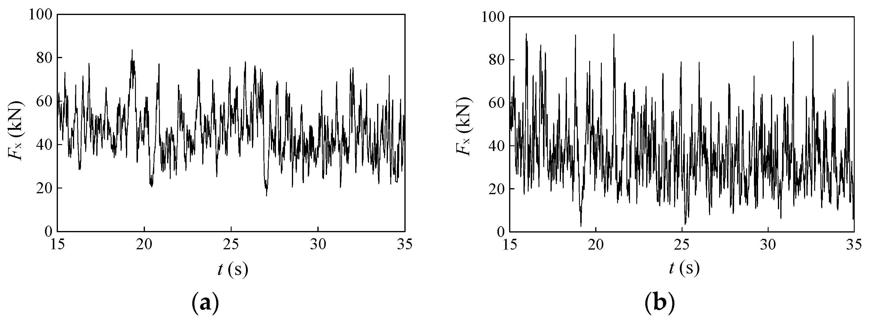
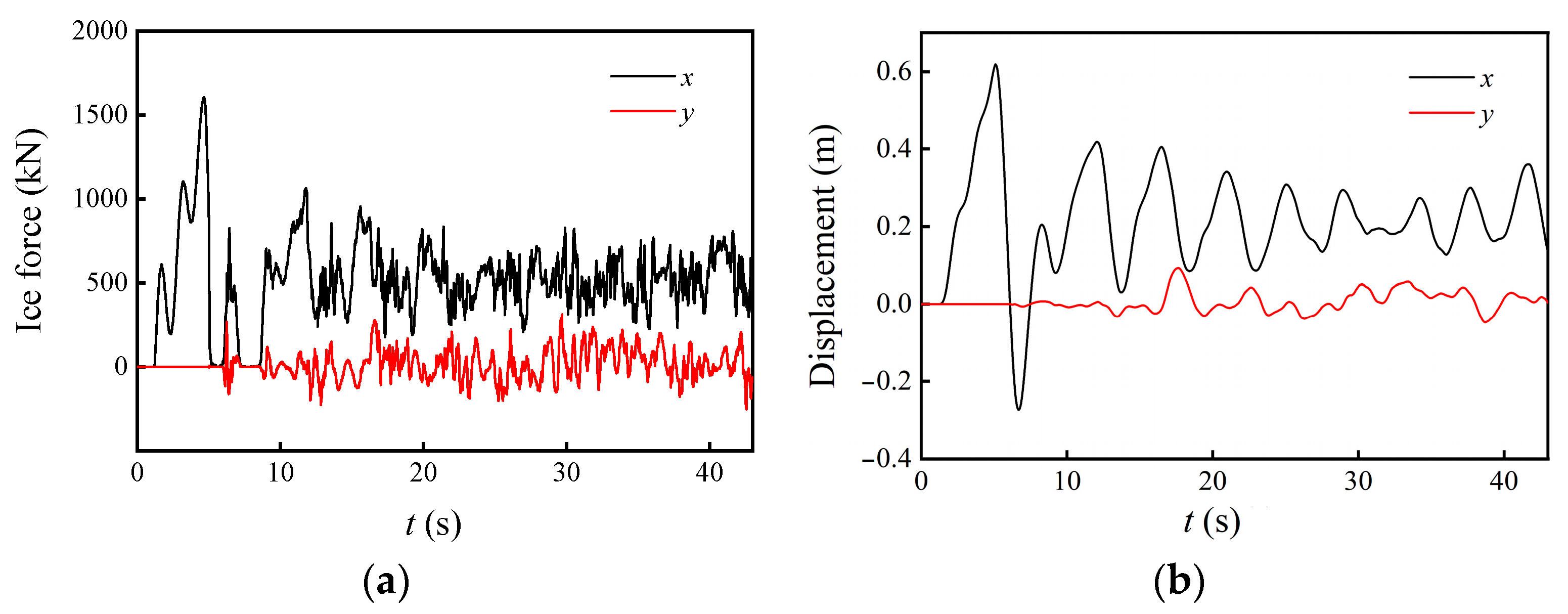
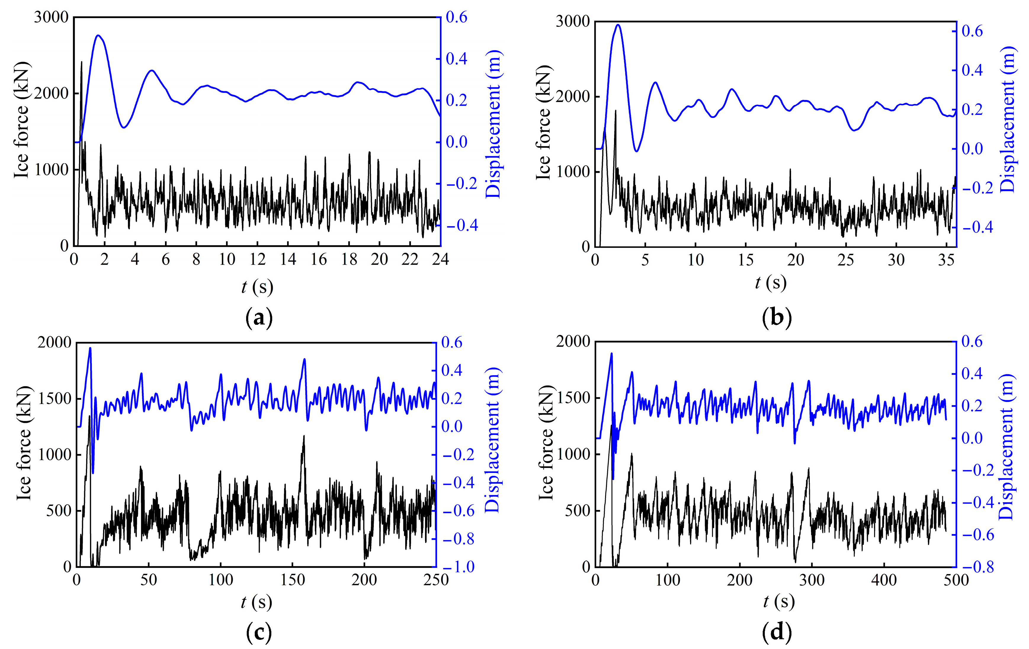
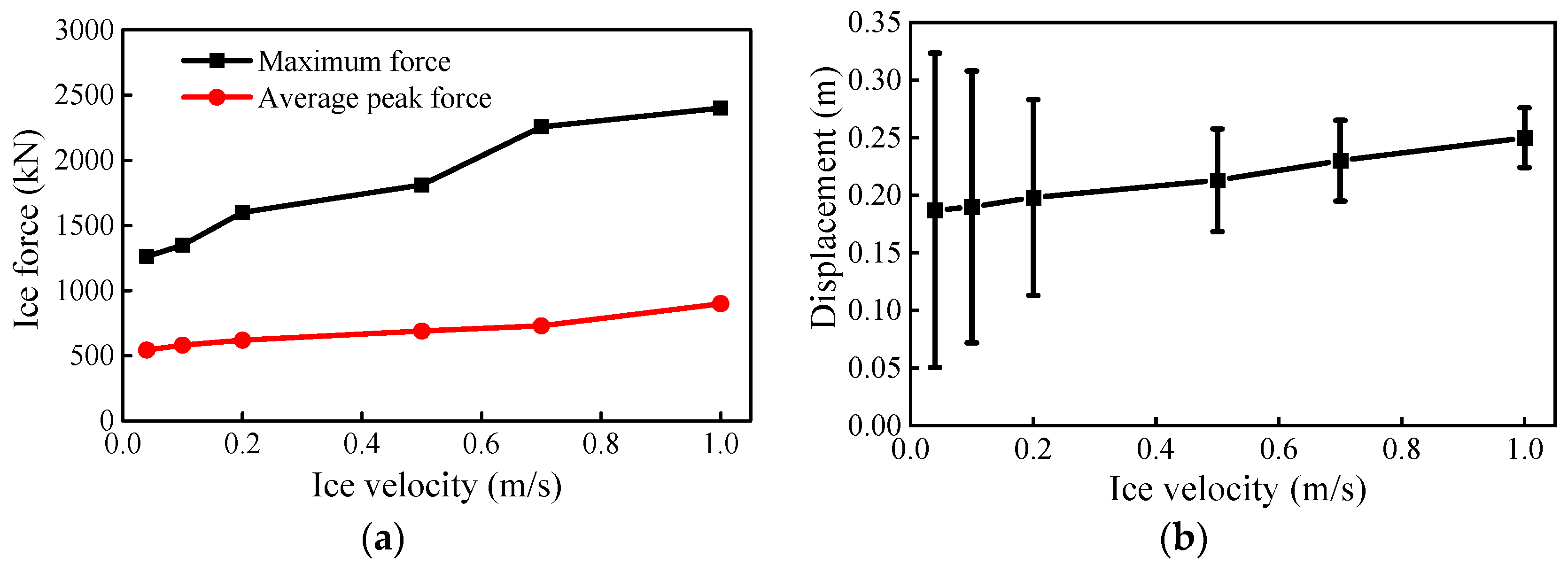
4.1. Influence of Ice Velocity
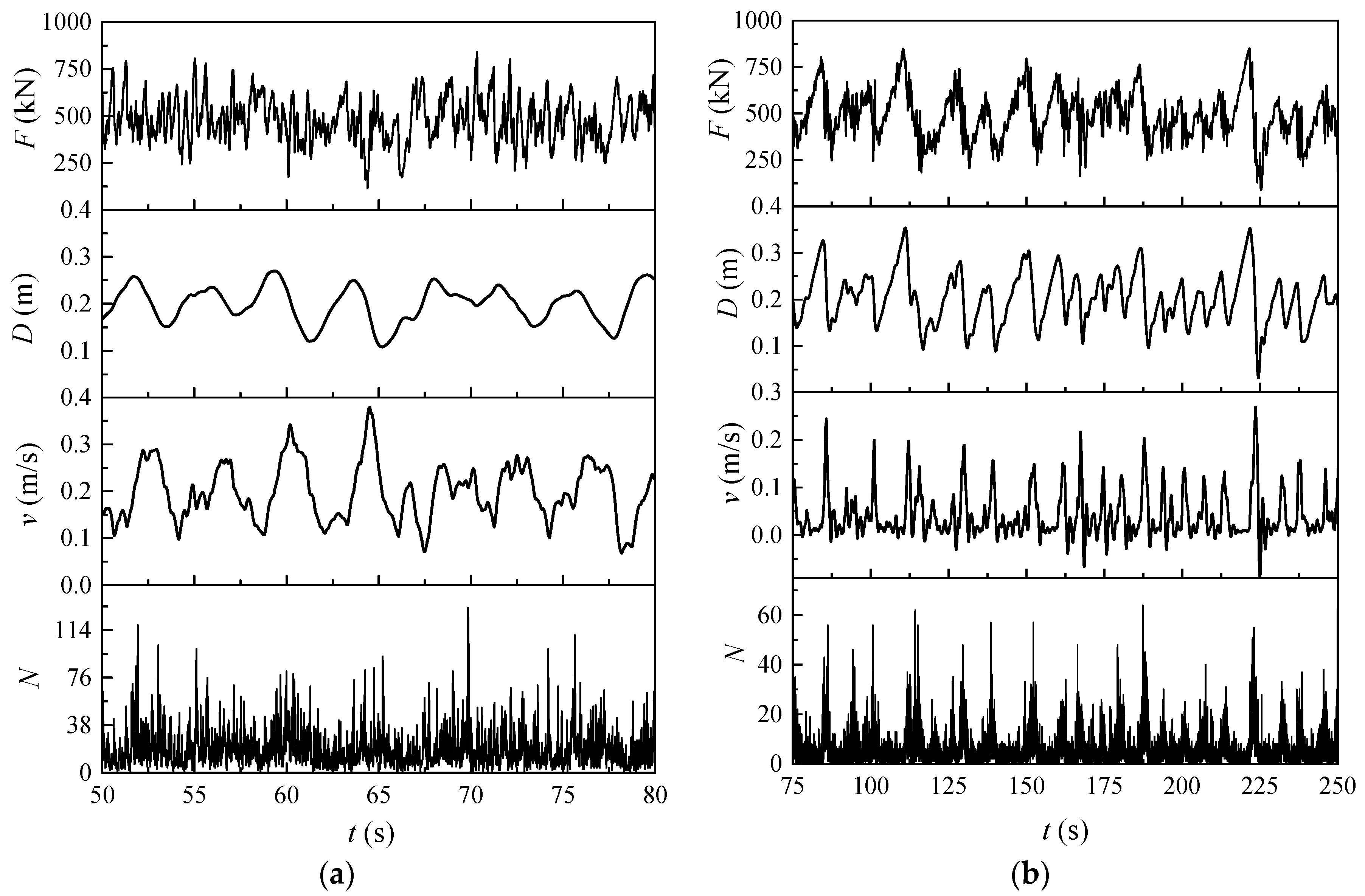
The primary structural parameters of the offshore wind turbine in the simulation are established based on its actual dimensions. Table 2 provides a comprehensive listing of the mass, stiffness, and other pertinent parameters. In the context of considering the interaction between the sea ice and the structures, it is important to note that the structure is treated as a rigid body, and any local deformations of the structure are disregarded. In terms of external loads acting on offshore wind turbines, these typically encompass the effects of waves and wind. However, when considering the substantial impact of the sea ice loads, this study omits the consideration of wind and wave loads. In the simulation, the structure exhibits three degrees of freedom, namely horizontal translation in both directions and vertical rotation. Consequently, this simulation is well-suited for calculating the vibration of the structure under the influence of ice loads.
In Figure 10, the interaction process between the sea ice and the wind turbine structure at an ice speed of 0.2 m/s is depicted. During this process, the sea ice experiences crushing failure, and the structure exhibits a vibrational response under the influence of the ice loads. Fragmented sea ice accumulates in front of the structure and is continuously pushed away by the subsequent sea ice, closely resembling the real-world phenomenon of sea ice crushing failure. To investigate the impact of ice velocity on the structural vibration, this study considers a range of ice velocities, varying from 0.04 m/s to 1.0 m/s. Figure 11 shows the ice force and displacement in the x and y directions when v = 0.2 m/s. It shows that the ice force and displacement in the x-direction are both larger than that in the y-direction. But the vibration in the y direction cannot be ignored because it affects the ice dynamics and breakage. The simulation results reveal that the sea ice consistently experiences crushing failure across different ice velocities, and the ice load exerts a sustained influence on the structure. However, the form of structural vibration exhibits significant variation. As the ice velocity increases, both the amplitude and frequency of structural vibration gradually decrease, as depicted in Figure 12. The direction of structural displacement consistent with the direction of ice velocity is positive, while the opposite is negative. To specifically explain the impact of ice velocity on ice load and structural vibration, the important data are summarized in Figure 13.
Figure 13a illustrates that both the maximum and mean values of the peak ice loads increase as the ice velocity rises. This behavior is attributed to the fact that, following the collision between the sea ice and the structure, the kinetic energy of the sea ice is converted into the structural kinetic energy and energy associated with the sea ice breaking. When the ice speed is elevated, the sea ice possesses greater kinetic energy, leading to an increase in the force acting on the structure. Nonetheless, it is important to note that at higher ice speeds, the fragmentation of the sea ice becomes more prevalent. As a result, the structural ice load does not increase at a proportionally significant rate with the escalation of the ice speed. In other words, the additional kinetic energy imparted by faster-moving sea ice does not translate into a commensurate increase in the structural ice load due to the concurrent fragmentation of the sea ice.
Figure 13b summarizes the mean vibration amplitude and mean structural displacement during the stable stage of the structural vibration under different ice velocities. It also highlights the changes in vibration amplitude of the structure at the mean point of the vibration displacement. The results reveal that as the ice velocity increases, the force exerted by the sea ice on the structure also increases, leading to a rise in the average displacement of the structure. However, a notable observation is that the amplitude of structural vibration decreases as the ice velocity increases. This phenomenon is connected to the changes in the types of structural vibration under different loading rates. When the ice speed is high, the structural displacement experiences minimal variation, and the structural vibration frequency is very low. On the other hand, when the ice speed is low, the structural vibration frequency significantly increases, resulting in periodic vibrations. When the frequency of the sea ice fragmentation aligns with the frequency of the structural vibration, the amplitude of the structural vibration increases. Consequently, the structural vibration at higher ice speeds can be characterized as random vibration, while lower ice speeds lead to larger structural vibrations with a periodic pattern. The vibrations of the sea ice at lower ice speeds can be classified as self-excited vibrations. The vibration patterns of the structures under the different ice velocities are influenced not only by factors such as their own mass and stiffness but also by the sustained action of the ice loads. The forthcoming analysis will compare these two vibration behaviors and elucidate the relationship between the sea ice fragmentation, the ice load, and the structural vibration to explain the mechanism of the self-excited vibration.

4.2. Discussions

In order to understand the influence of ice velocity on the forms of structural vibration, a comparison was made between the ice load (F), the structural vibration displacement (D), the relative motion velocity (v) between sea ice and the structure, and the number of bond failures of spherical elements within sea ice (N) under two different ice velocity conditions: 0.2 m/s and 0.04 m/s, as depicted in Figure 14. When the ice speed is 0.2 m/s, there is no discernible interaction between the changes in these four parameters; their behaviors appear independent of each other. However, when the ice speed is reduced to 0.04 m/s, the changes in all four parameters exhibit periodicity, and their change periods are nearly identical. This observation indicates that, at low ice speeds, the structural vibration and the ice load exhibit mutual influence. In other words, as the structural vibrations intensify, they affect the process of sea ice fragmentation, and in turn, the structural vibration is impacted by the variations in the ice loads. On the contrary, at high ice speeds, the structural vibrations and ice load changes occur independently, and the structural vibrations do not interfere with the process of sea ice fragmentation. This suggests that the mechanism of self-excited vibration is more pronounced at low ice velocities, where the vibrations of the structure and the sea ice are intertwined and synchronized, resulting in a periodic vibration pattern. At high ice velocities, the structural vibrations are more likely to follow a random vibration pattern.
The presence of synchronous periodicity is closely linked to the sea ice fragmentation process. When the ice velocity is 0.2 m/s, the relative motion velocity between the sea ice and the structure consistently remains greater than zero, and the ice velocity always exceeds the velocity of the structure. In this scenario, the sea ice continuously exerts a driving force on the structure. The sustained interaction leads to a consistently high number of bond failures, indicating that the sea ice experiences ongoing brittle fragmentation at high ice velocities. In contrast, when the ice speed is reduced to 0.04 m/s, the relative motion velocity between the sea ice and the structure approaches zero or even becomes negative. This suggests that the structure can detach from the sea ice. When pushed by the sea ice, the structure can attain significant movement speed, which results in an increased number of bond failures, intensifying the sea ice damage and promoting brittle failure. The front portion of the sea ice sustains severe damage, and the structural movement speed accelerates, causing the sea ice to gradually detach from the structure and lose its interaction force. Simultaneously, the number of bond failures decreases, or even falls to zero, and the rate of the sea ice failure slows down, showing characteristics of ductile failure. Significant differences are observed in the sea ice fragmentation process at different ice velocities. At high ice speeds, the sea ice consistently experiences brittle failure, while at low ice speeds, the sea ice transitions from brittle to ductile failure. The failure process of the sea ice at low ice speeds is relatively complex and requires further detailed examination and discussion.
The variation process of an ice load cycle at an ice speed of 0.04 m/s is further amplified in Figure 15, and it is presented alongside the structural displacement, the relative motion velocity between the sea ice and the structure, and the number of unit bond failures within the same cycle. This illustration aims to provide insight into the detailed dynamics during the ice load cycle. The cycle can be divided into three distinct stages: the loading stage, load transition stage, and unloading stage. Analyzing these stages necessitates an understanding of the sea ice fragmentation process, as represented in Figure 16. In this figure, colors are used to denote the interaction forces between individual elements, and auxiliary dashed lines are utilized to indicate changes in the structural position. The specific analysis process is as follows.
Loading stage (from t = 216.0 s to t = 221.5 s): As shown in Figure 15, taking t = 216.0 s as the initial point of the structural motion cycle, the relative motion velocity between the sea ice and the structure is zero. During the loading stage, the displacement of the structure gradually increases under the push of the sea ice, and the ice load increases. However, the relative velocity between the structure and the sea ice is always zero, and the number of bonding failures also varies near a small value. From Figure 16a,b, it can be seen that at this time, there is less sea ice fracture and the structure is pushed to move together and always maintains close contact. At the same time, the force acting on the elements at the front of the sea ice gradually increases, and the ice load on the structure also gradually increases. From the number of bonding failures and the macroscopic effect of sea ice fragmentation and accumulation, it can be seen that at this stage, due to the relatively low movement speed between the sea ice and the structure, there is no significant damage to the sea ice, and only cumulative cracks are generated inside it. Its failure mode belongs to ductile failure.
Load transition stage (from t = 221.5 s to t = 222.5 s): In this stage, the vertical structure moves forward under the push of the sea ice to reach the maximum displacement position, and the ice load reaches the maximum value. Due to the decrease in the speed of movement of the structure, the relative velocity between the sea ice and the structure begins to increase. Meanwhile, the increase in the loading rate of the structure on the sea ice leads to a gradual increase in the number of bonding failures. From Figure 16c, it can be seen that there is an increase in the sea ice that has been compressed and broken at this time, and the stacking height in front of the structure also increases. It can be seen that during this process, the structural stiffness changes the speed of the structural motion, thereby affecting the failure process of the sea ice. The failure mode of the sea ice is usually influenced by the loading rate. When the loading rate is low, it is ductile failure, and while when the loading rate is high, it is brittle failure. At this stage, the loading rate is increasing, and the fragmentation of the sea ice also intensifies, indicating that the failure mode of the sea ice has shifted from ductile failure to brittle failure.
Unloading stage (from t = 222.5 s to t = 224.5 s): After the structural movement reaches the maximum displacement, it quickly rebounds, and the rebound process manifests as accelerating first and then decelerating. When the structure accelerates rebound, the relative velocity with the sea ice also rapidly increases, and a large amount of compression occurs at the front end of the ice sheet. When the displacement of the structure reaches its maximum value, the number of unit bond failures also reaches its maximum. At this point, the sea ice exhibits brittle failure, and the front end of the ice sheet cannot maintain a significant contact force with the structure due to fragmentation, resulting in a rapid decrease in the ice load. When the structure rebounds at a reduced speed, the number of unit bond failures begins to decrease, while the ice load continues to decrease but decreases slowly and tends to stabilize. When the structure rebounds to the minimum position, the ice load decreases to the minimum value, the relative velocity between the sea ice and the structure approaches zero, and the number of bonding failures also decreases to a smaller value. At this point, the interaction between the sea ice and the structure completes a periodic change.
The analysis reveals that during the periodic vibration of the structure, the nature of the sea ice failure varies depending on the relative velocity between the sea ice and the structure. These observations can be summarized as follows.
  • Ductile crushing failure: When the relative velocity between the sea ice and the structure is relatively small, the sea ice undergoes ductile crushing failure. In this scenario, the interaction between the sea ice and the structure occurs in a manner that leads to ductile failure characteristics. The ice tends to accumulate and crack, and its failure mode is ductile.
  • Brittle crushing failure: Conversely, when the relative velocity between the sea ice and the structure is relatively high, the sea ice undergoes brittle crushing failure. This high relative velocity leads to a more brittle failure mode, where the ice fragmentation is rapid, and the front end of the ice sheet loses contact with the structure.
  • Ductile-brittle transition: In certain transition regions where the relative velocities are intermediate, a ductile-brittle transition can occur. This implies that the failure mode of the sea ice in these areas may exhibit characteristics of both ductile and brittle compression.
These observations highlight the dynamic nature of the sea ice failure during the interaction with the structures. Sea ice failure depends not only on its inherent strength but is also significantly influenced by the structural stiffness and vibration. Moreover, the nature of the structural vibration, particularly during steady-state vibrations, has a feedback effect on the ice load. This implies that, under specific conditions and lower ice speeds, the structural vibration exhibits self-excited characteristics, where the structural motion and sea ice failure mutually influence one another, leading to a sustained and dynamic interaction.
The analysis suggests that the steady-state vibration of a structure under the influence of the sea ice can lead to significant structural damage and should be avoided in engineering practice. To prevent or minimize the occurrence of steady-state vibration, it is important to address the key factor contributing to this type of vibration–ductile crushing of the sea ice. Steady-state vibration of the structures is often associated with ductile failure of the sea ice. Ductile failure involves the slow accumulation and gradual cracking of the sea ice. The structural motion and vibration are sustained due to the slow, continuous interaction with the sea ice. Ductile failure of the sea ice is influenced by the loading rate (relative velocity between sea ice and structure) and the shape of the structure. A higher loading rate, which typically occurs at lower ice speeds, is more likely to induce ductile failure. To mitigate ductile failure and prevent steady-state vibration, one effective strategy is to modify the structural surface by adding rib plates or other features. These rib plates can be strategically designed to induce radial cracks at the front end of the ice sheet when in contact with the structure. The concept of using rib plates to control the interaction between the sea ice and the structures is to disrupt the sustained, ductile failure mode of the sea ice. By inducing cracks and altering the manner in which the sea ice accumulates and fails, the structure can avoid the detrimental effects of steady-state vibration and the potential for damage. Hence, controlling ductile crushing of the sea ice by modifying the structural shape with rib plates or similar features is a practical engineering approach to prevent steady-state vibrations and minimize structural damage during interactions with sea ice.

5. Conclusions

This paper investigates sea ice failure modes and structural vibration at different ice speeds, shedding light on the impact of ice-induced vibration. When the ice speed is fast, the sea ice undergoes random brittle failure, resulting in randomness of the ice load and the structural vibration. When the ice speed is slow, the breaking process of the sea ice undergoes a ductile-brittle transition with periodicity. The failure mode of the sea ice leads to periodic changes in the ice load and the structural vibration, indicating that the structure undergoes self-excited vibration at this time. Moreover, when self-excited vibration occurs in OWTs, the vibration amplitude is larger and the vibration frequency is higher, which poses the greatest harm to the structural strength. There is a coupling relationship between the sea ice failure mode and the structural vibration, which interact with each other. Therefore, limiting the ductile-brittle transition of the sea ice can become a way to avoid the occurrence of structural self-excited vibration, such as adding anti-ice cone structures. Understanding and managing self-excited vibrations in such systems are crucial for the safe and effective operation of offshore wind turbine structures in cold regions.

Author Contributions

Conceptualization and methodology, X.L. and S.J.; methodology, X.L. and S.J.; validation, X.L. and L.L.; writing and editing, X.L. All authors have read and agreed to the published version of the manuscript.

Funding

This research was funded by the National Natural Science Foundation of China (Grant Nos. 52001041, 12102083) and the Fundamental Research Funds for the Central Universities (Grant No. 3132022114).

Institutional Review Board Statement

Not applicable.

Informed Consent Statement

Not applicable.

Data Availability Statement

The data presented in this study are available on request from the corresponding author.

Acknowledgments

The authors would like to thank all colleagues and reviewers who provided assistance and advice to this study.

Conflicts of Interest

The authors declare no conflict of interest.

References

  1. Yu, Y.; Wu, S.; Yu, J.; Xu, Y.; Song, L.; Xu, W. A hybrid multi-criteria decision-making framework for offshore wind turbine selection: A case study in China. Appl. Energy 2022, 328, 120173. [Google Scholar] [CrossRef]
  2. Wei, S. Offshore Wind Turbine-Ice Interactions. In Encyclopedia of Ocean Engineering; Cui, W., Fu, S., Hu, Z., Eds.; Springer: Singapore, 2020. [Google Scholar]
  3. Swenson, L.; Gao, L.; Hong, J.; Shen, L. An efficacious model for predicting icing-induced energy loss for wind turbines. Appl. Energy 2022, 305, 117809. [Google Scholar] [CrossRef]
  4. Barstad, I.; Sorteberg, A.; Mesquita, M.S. Present and future offshore wind power potential in northern Europe based on downscaled global climate runs with adjusted SST and sea ice cover. Renew. Energy 2012, 44, 398–405. [Google Scholar] [CrossRef]
  5. Wang, X.; Zeng, X.; Yang, X.; Li, J. Feasibility study of offshore wind turbines with hybrid monopile foundation based on centrifuge modeling. Appl. Energy 2018, 209, 127–139. [Google Scholar] [CrossRef]
  6. Dinh, Q.V.; Doan, Q.V.; Ngo-Duc, T.; Dinh, V.N.; Duc, N.D. Offshore wind resource in the context of global climate change over a tropical area. Appl. Energy 2022, 308, 118369. [Google Scholar] [CrossRef]
  7. Nord, T.S.; Samardzija, I.; Hendrikse, H.; Bjerkås, M.; Høyland, K.V.; Li, H. Ice-induced vibrations of the Norströmsgrund lighthouse. Cold Reg. Sci. Technol. 2018, 155, 237–251. [Google Scholar] [CrossRef]
  8. Huang, S.; Huang, M.; Lyu, Y.; Xiu, L. Effect of sea ice on seismic collapse-resistance performance of wind turbine tower based on a simplified calculation model. Eng. Struct. 2021, 227, 111426. [Google Scholar] [CrossRef]
  9. Wang, X.; Zeng, X.; Yang, X.; Li, J. Seismic response of offshore wind turbine with hybrid monopile foundation based on centrifuge modelling. Appl. Energy 2019, 235, 1335–1350. [Google Scholar] [CrossRef]
  10. Frederking, R.; Sudom, D. Maximum ice force on the Molikpaq during the April 12, 1986 event. Cold Reg. Sci. Technol. 2006, 46, 147–166. [Google Scholar] [CrossRef]
  11. Wang, S.; Yue, Q.; Zhang, D. Ice-induced non-structure vibration reduction of jacket platforms with isolation cone system. Ocean Eng. 2013, 70, 118–123. [Google Scholar] [CrossRef]
  12. Yue, Q.; Qu, Y.; Bi, X.; Kärnä, T. Ice force spectrum on narrow conical structures. Cold Reg. Sci. Technol. 2007, 49, 161–169. [Google Scholar] [CrossRef]
  13. Nord, T.S.; Øiseth, O.; Lourens, E.M. Ice force identification on the Norströmsgrund lighthouse. Comput. Struct. 2016, 169, 24–39. [Google Scholar] [CrossRef]
  14. ISO19906; Petroleum and Natural Gas Industries—Arctic Offshore Structures. International Organization for Standardization: Geneva, Switzerland, 2010.
  15. Sodhi, D.S. A theoretical model for Ice-Structure Interaction. In Proceedings of the OMAE-94 Conference; ASME: New York, NY, USA, 1994; Volume IV, pp. 29–34. [Google Scholar]
  16. Hendrikse, H.; Metrikine, A. Interpretation and prediction of ice induced vibrations based on contact area variation. Int. J. Solids Struct. 2015, 75–76, 336–348. [Google Scholar] [CrossRef]
  17. Ji, X.; Oterkus, E. A dynamic ice-structure interaction model for ice-induced vibrations by using van der pol equation. Ocean Eng. 2016, 128, 147–152. [Google Scholar] [CrossRef]
  18. Abramian, A.K.; Vakulenko, S.A.; Horssen, W.T.V. A mathematical analysis of an extended model describing sea ice-induced frequency lock-in for vertically sided offshore structures. Nonlinear Dyn. 2022, 107, 683–699. [Google Scholar] [CrossRef]
  19. Snyder, S.A.; Schulson, E.M.; Renshaw, C.E. Effects of prestrain on the ductile-to-brittle transition of ice. Acta Mater. 2016, 108, 110–127. [Google Scholar] [CrossRef]
  20. Seidela, M.; Hendrikse, H. Analytical assessment of sea ice-induced frequency lock-in for offshore wind turbine monopiles. Mar. Struct. 2018, 60, 87–100. [Google Scholar] [CrossRef]
  21. Gagnon, R. Spallation-based numerical simulations of ice-induced vibration of structures. Cold Reg. Sci. Technol. 2022, 194, 103465. [Google Scholar] [CrossRef]
  22. Schulson, E.M. Brittle failure of ice. Eng. Fract. Mech. 2001, 68, 1839–1887. [Google Scholar] [CrossRef]
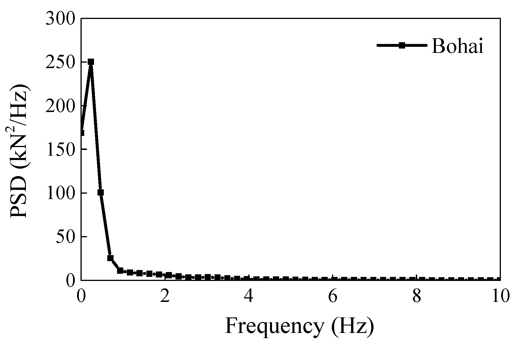
  23. Zhang, D.Y.; Wang, G.J.; Yue, Q.J. Evaluation of ice-induced fatigue life for a vertical offshore structure in the Bohai Sea. Cold Reg. Sci. Technol. 2018, 154, 103–110. [Google Scholar] [CrossRef]
  24. Zhu, B.; Sun, C.; Jahangiri, V. Characterizing and mitigating ice-induced vibration of monopile offshore wind turbines. Ocean Eng. 2021, 219, 108406. [Google Scholar] [CrossRef]
  25. Dempsey, J.P.; Palmer, A.C.; Sodhi, D.S. High pressure zone formation during compressive ice failure. Eng. Fract. Mech. 2001, 68, 1961–1974. [Google Scholar] [CrossRef]
  26. Tian, Y.; Huang, Y. The dynamic ice loads on conical structures. Ocean Eng. 2013, 59, 37–46. [Google Scholar] [CrossRef]
  27. Qu, Y.; Yue, Q.; Bi, X.; Kärnä, T. A random ice force model for narrow conical structures. Cold Reg. Sci. Technol. 2006, 45, 148–157. [Google Scholar]
  28. Xue, Y.Z.; Liu, R.W.; Li, Z.; Han, D.F. A review for numerical simulation methods of ship–ice interaction. Ocean Eng. 2020, 215, 107853. [Google Scholar] [CrossRef]
  29. Banerjee, S.; Agarwal, R. Transient reacting flow simulation of spouted fluidized bed for coal-direct chemical looping combustion with different Fe-based oxygen carriers. Appl. Energy 2015, 160, 552–560. [Google Scholar] [CrossRef]
  30. Gaviño, D.; Cortés, E.; García, J.; Calderón-Vásquez, I.; Cardemil, J.; Estay, D.; Barraza, R. A discrete element approach to model packed bed thermal storage. Appl. Energy 2022, 325, 119821. [Google Scholar] [CrossRef]
  31. Feng, Y.H.; Dai, Y.J.; Wang, R.Z.; Ge, T.S. Insights into desiccant-based internally-cooled dehumidification using porous sorbents: From a modeling viewpoint. Appl. Energy 2022, 311, 118732. [Google Scholar] [CrossRef]
  32. Shen, H.H.; Hibler, W.D.; Leppäranta, M. On applying granular flow theory to a deforming broken ice field. Acta Mech. 1986, 63, 143–160. [Google Scholar] [CrossRef]
  33. Wang, C.; Xu, Z.; Koeppel, B. A discrete element model simulation of structure and bonding at interfaces between cathode and cathode contact paste in solid oxide fuel cells. Renew. Energy 2020, 157, 998–1007. [Google Scholar] [CrossRef]
  34. Li, Z.; Yu, J.; Yue, Q.; Yu, Y.; Guo, X. Study on meso-mechanical mechanism and energy of moisture content on densification of salix psammophila particles. Renew. Energy 2023, 205, 1071–1081. [Google Scholar] [CrossRef]
  35. Tuhkuri, J.; Polojärvi, A. A review of discrete element simulation of ice–structure interaction. Phil. Trans. R. Soc. A 2018, 376, 20170335. [Google Scholar] [CrossRef] [PubMed]
  36. Long, X.; Liu, S.; Ji, S. Discrete element modelling of relationship between ice breaking length and ice load on conical structure. Ocean Eng. 2020, 201, 107152. [Google Scholar] [CrossRef]
  37. Sun, S.; Shen, H.H. Simulation of pancake ice load on a circular cylinder in a wave and current field. Cold Reg. Sci. Technol. 2012, 78, 21–39. [Google Scholar] [CrossRef]
  38. Pradana, M.R.; Qian, X.; Ahmed, A. Efficient discrete element simulation of managed ice actions on moored floating platforms. Ocean Eng. 2019, 190, 106483. [Google Scholar] [CrossRef]
  39. Brædstrup, C.F.; Damsgaard, A.; Egholm, D.L. Ice-sheet modelling accelerated by graphics cards. Comput. Geosci. 2014, 72, 210–220. [Google Scholar] [CrossRef]
  40. Jou, O.; Celigueta, M.A.; Latorre, S.; Arrufat, F.; Oñate, E. A bonded discrete element method for modeling ship–ice interactions in broken and unbroken sea ice fields. Comput. Part. Mech. 2019, 6, 739–765. [Google Scholar] [CrossRef]
  41. Di, S.; Xue, Y.; Wang, Q.; Bai, X. Discrete element simulation of ice loads on narrow conical structures. Ocean Eng. 2017, 146, 282–297. [Google Scholar] [CrossRef]
  42. Guo, L.; Latham, J.P.; Xiang, J. Numerical simulation of breakages of concrete armour units using a three-dimensional fracture model in the context of the combined finite-discrete element method. Comput. Struct. 2015, 146, 117–142. [Google Scholar] [CrossRef]
  43. Ma, G.; Zhou, W.; Chang, X.L.; Chen, M.X. A hybrid approach for modeling of breakable granular materials using combined finite-discrete element method. Granul. Matter 2016, 18, 7. [Google Scholar] [CrossRef]
  44. Mcdowell, G.R.; Bolton, M.D.; Robertson, D. The fractal crushing of granular materials. J. Mech. Phys. Solids 1996, 44, 2079–2102. [Google Scholar] [CrossRef]
  45. Lu, W.; Lubbad, R.; Løset, S. Simulating ice-sloping structure interactions with the cohesive element method. J. Offshore Mech. Arct. Eng. 2014, 136, 031501. [Google Scholar] [CrossRef]
  46. Potyondy, D.O.; Cundall, P.A. A bonded-particle model for rock. Int. J. Rock Mech. Min. Sci. 2004, 41, 1329–1364. [Google Scholar] [CrossRef]
  47. Wang, Y.; Mora, P. Macroscopic elastic properties of regular lattices. J. Mech. Phys. Solids 2008, 56, 3459–3474. [Google Scholar] [CrossRef]
  48. Pradana, M.R.; Qian, X. Bridging local parameters with global mechanical properties in bonded discrete elements for ice load prediction on conical structures. Cold Reg. Sci. Technol. 2020, 173, 102960. [Google Scholar] [CrossRef]
  49. Morgan, D.; Sarracino, R.; McKenna, R.; Thijssen, J.W. Simulations of ice rubbling against conical structures using 3D DEM. In Proceedings of the 23rd International Conference on Port and Ocean Engineering under Arctic Conditions (POAC ‘15), Trondheim, Norway, 14–18 June 2015. [Google Scholar]
  50. Di, S.; Xue, Y.; Bai, X.; Wang, Q. Effects of model size and particle size on the response of sea-ice samples created with a hexagonal-close-packing pattern in discrete- element method simulations. Particuology 2018, 36, 106–113. [Google Scholar] [CrossRef]
  51. Long, X.; Ji, S.; Wang, Y. Validation of microparameters in discrete element modeling of sea ice failure process. Part. Sci. Technol. 2019, 37, 550–559. [Google Scholar] [CrossRef]
  52. Zhou, Q.; Xu, W.J.; Liu, G.Y. A contact detection algorithm for triangle boundary in GPU-based DEM and its application in a large-scale landslide. Comput. Geotech. 2021, 138, 104371. [Google Scholar] [CrossRef]
  53. Williams, J.R.; O’connor, R. A linear complexity intersection algorithm for discrete element simulation of arbitrary geometries. Eng. Comput. 1995, 12, 185–201. [Google Scholar] [CrossRef]
  54. Huang, P.; Ding, Y.; Miao, Q.; Sang, G.; Jia, M. An improved contact detection algorithm for bonded particles based on multi-level grid and bounding box in DEM simulation. Powder Technol. 2020, 374, 577–596. [Google Scholar] [CrossRef]
  55. Hopkins, M.; Shen, H. Simulation of pancake-ice dynamics in a wave field. Ann. Glaciol. 2001, 33, 355–360. [Google Scholar] [CrossRef]
  56. Govender, N.; Wilke, D.N.; Kok, S.; Els, R. Development of a convex polyhedral discrete element simulation framework for NVIDIA Kepler based GPUs. J. Comput. Appl. Math. 2014, 270, 386–400. [Google Scholar] [CrossRef]
  57. Raji, A.; Favier, J. Discrete element modelling of the compression of an oil-seed bed. In Proceedings of the ASAE International Conference, Toronto, ON, Canada, 18–21 July 1999. [Google Scholar]
  58. Long, X.; Liu, L.; Liu, S.; Ji, S. Discrete element analysis of high-pressure zones of sea ice on vertical structures. J. Mar. Sci. Eng 2021, 9, 348. [Google Scholar] [CrossRef]
  59. Benzeggagh, M.L.; Kenane, M. Measurement of Mixed-Mode Delamination Fracture Toughness of Unidirectional Glass/Epoxy Composites with Mixed-Mode Bending Apparatus. Compos. Sci. Technol. 1996, 56, 439–449. [Google Scholar] [CrossRef]
  60. Ma, G.; Zhou, W.; Chang, X.L. Modeling the particle breakage of rockfill materials with the cohesive crack model. Comput. Geotech. 2014, 61, 132–143. [Google Scholar] [CrossRef]
  61. Camanho, P.P.; Davila, C.G.; Moura, M.F.D. Numerical Simulation of Mixed-Mode Progressive Delamination in Composite . Mater. J. Compos. Mater. 2003, 37, 1415–1438. [Google Scholar] [CrossRef]
Figure 1. DEM setup of the interaction between level ice and monopile OWT.
Jmse 11 02153 g001
Figure 2. Parallel bond model for spherical elements.
Jmse 11 02153 g002
Figure 3. Fracture criterion considering damage.
Jmse 11 02153 g003
Figure 4. Crushing failure of sea ice on the vertical pile structure in field data of the Bohai Sea.
Jmse 11 02153 g004
Figure 5. DEM simulation of ice crushing failure under different bond-failure models: (a) hybrid fracture criterion with damage; (b) tensile-shear fracture criterion.
Jmse 11 02153 g005
Figure 6. Time history of ice load in field data of the Bohai Sea.
Jmse 11 02153 g006
Figure 7. DEM simulation of time history of ice load under different fracture criterion: (a) hybrid fracture criterion with damage; (b) tensile-shear fracture criterion.
Jmse 11 02153 g007
Figure 8. Spectrum analysis of ice load in field data of Bohai Sea.
Jmse 11 02153 g008
Figure 9. DEM simulation of spectrum analysis of ice load under different fracture criterion: (a) hybrid fracture criterion with damage; (b) tensile-shear fracture criterion.
Jmse 11 02153 g009
Figure 10. The failure process of sea ice under the interaction of wind turbine structure: (a) t = 0 s; (b) t = 70.0 including the entire view (left) and locally enlarged view (right).
Jmse 11 02153 g010
Figure 11. The ice force and displacement in x and y directions when v = 0.2 m/s: (a) ice force; (b) displacement.
Jmse 11 02153 g011
Figure 12. Structural ice load and vibration response under different ice velocities: (a) v =1.0 m/s; (b) v = 0.5 m/s; (c) v = 0.1 m/s; (d) v = 0.04 m/s.
Jmse 11 02153 g012
Figure 13. Effect of ice velocity on structural ice load and amplitude: (a) ice load; (b) structural amplitude.
Jmse 11 02153 g013
Figure 14. Number of failures between elements at different ice velocity versus time: (a) t = 0.2 m/s; (b) t = 0.04 m/s.
Jmse 11 02153 g014
Figure 15. Relationship between ice load, structural vibration, relative velocity between sea ice and structure and element bonding failure times during self-excited vibration of the structure.
Jmse 11 02153 g015
Figure 16. Crushing failure process of the interaction between sea ice and vertical pile structure: (a) t = 216 s; (b) t = 220 s; (c) t = 222 s; (d) t = 223 s. The plus sign denotes the center position of the structure.
Jmse 11 02153 g016
Table 1. DEM parameters of the interaction between sea ice and vertical pile structure.
DefinitionSymbolValue
Density of sea ice ρ i 920 kg/m3
Density of seawater ρ w 1035 kg/m3
Sample size L × W × H 20 m × 10 m × 0.18 m
Element size D 4.48 cm
Normal stiffness k n 1.72 × 10⁷ N/m
Shear stiffness k s 1.72 × 10⁶ N/m
Internal friction μ b 0.2
Normal bonding strength σ b n 0.5 MPa
Shear bonding strength σ b s 0.5 MPa
Sea ice velocity V 0.2 m/s
Drag coefficient C d 0.05
Element number N p 608,790
Table 2. The main structural parameters of the offshore wind turbine.
DefinitionsValues
Structure mass7.69 × 105 kg
Structure stiffness2.42 × 106 N/m
Structure damping0.15
Natural frequency of structure1.77 Hz
Structure diameter in waterline5.50 m
Sea ice thickness0.30 m
Element size0.11 m
Bonding strength1.01 MPa
Disclaimer/Publisher’s Note: The statements, opinions and data contained in all publications are solely those of the individual author(s) and contributor(s) and not of MDPI and/or the editor(s). MDPI and/or the editor(s) disclaim responsibility for any injury to people or property resulting from any ideas, methods, instructions or products referred to in the content.

