
Numerical Study of Turbulent Wake of Offshore Wind Turbines and Retention Time of Larval Dispersion


Abstract
:1. Introduction
2. Model Description
2.1. Hydrodynamic Model
2.1.1. Governing Equations
2.1.2. Boundary Conditions and Initial Conditions
2.2. Lagrangian Model
2.2.1. Governing Equations
2.2.2. Boundary Conditions and Initial Conditions
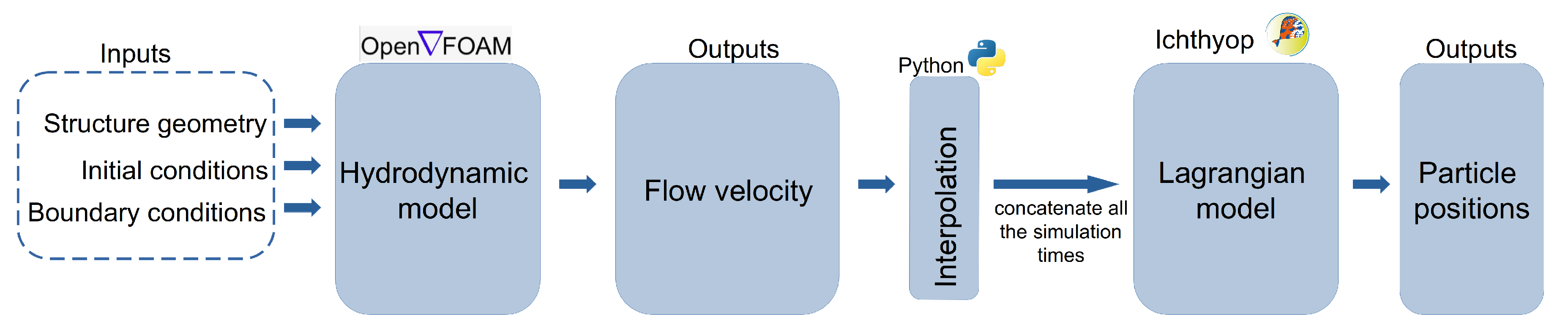
2.3. Models’ Coupling
3. A Laboratory Test Case
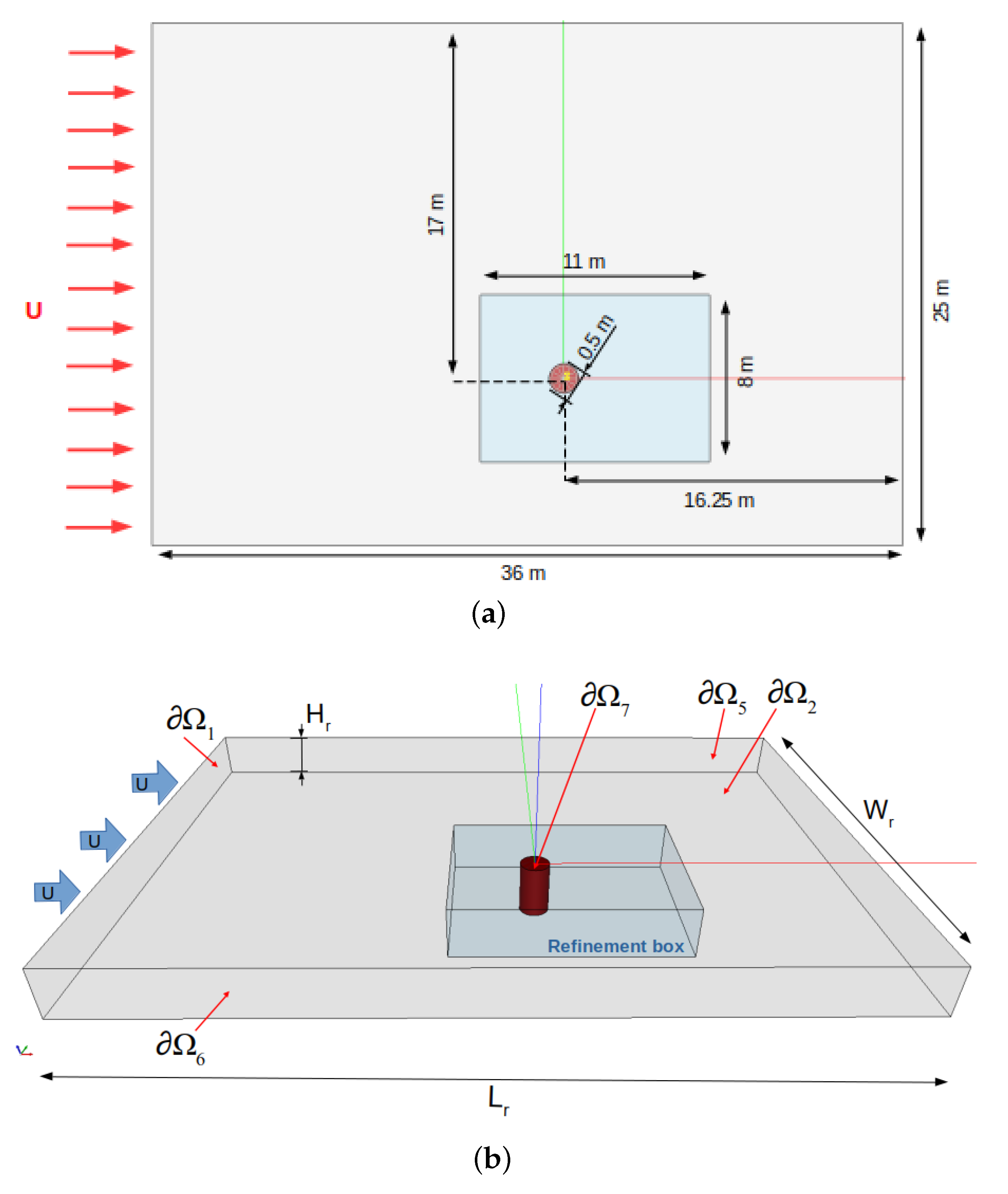
3.1. Domain Geometry
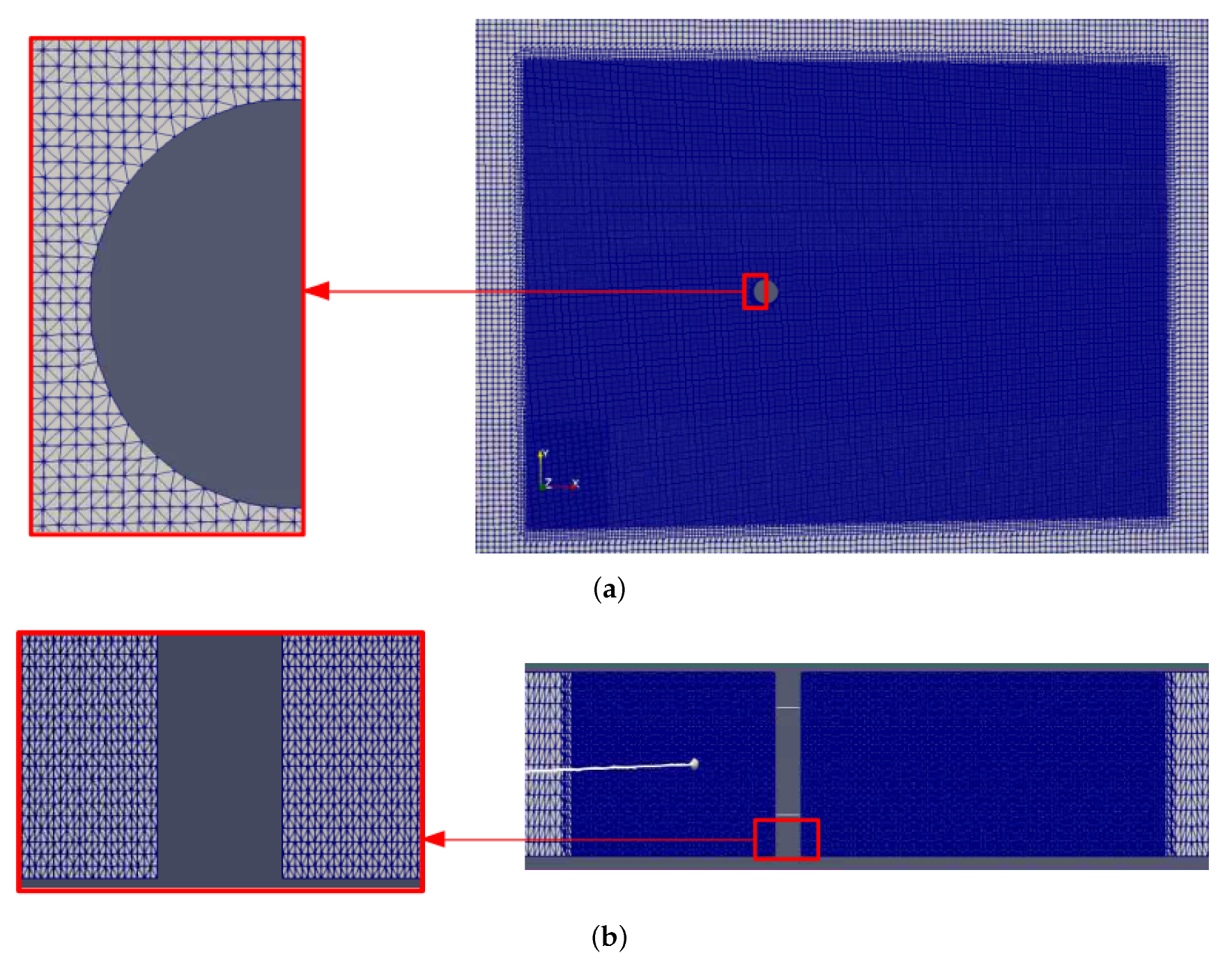
3.2. Mesh
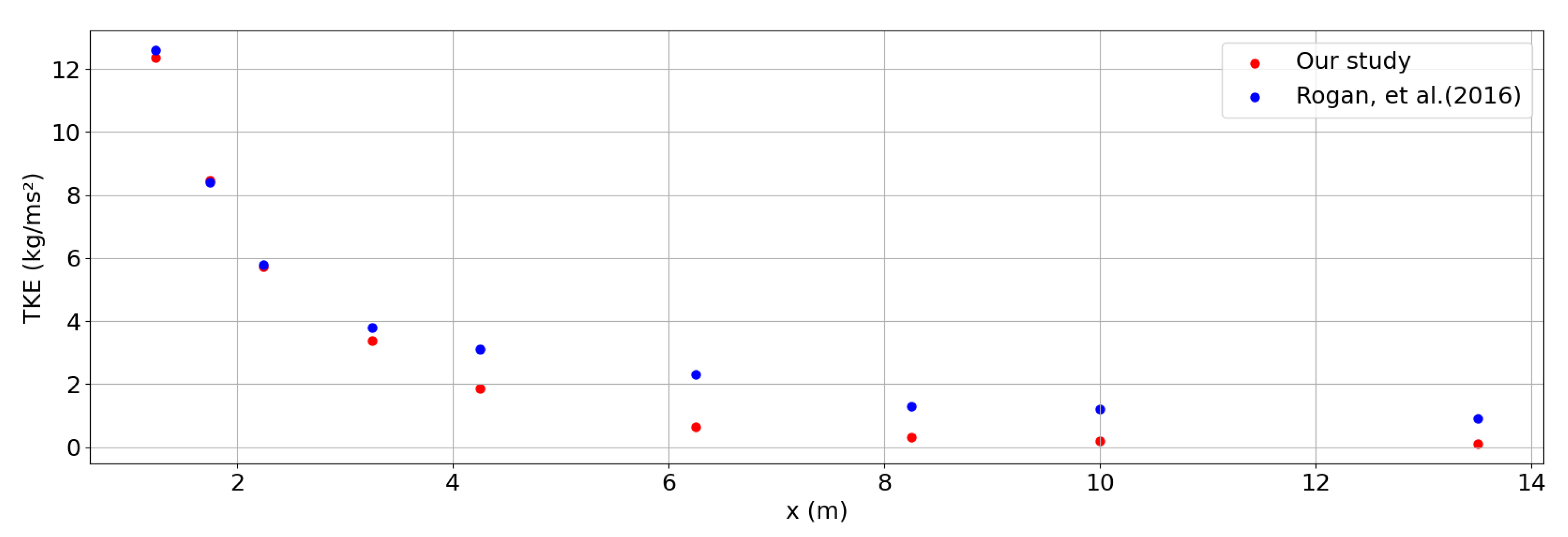
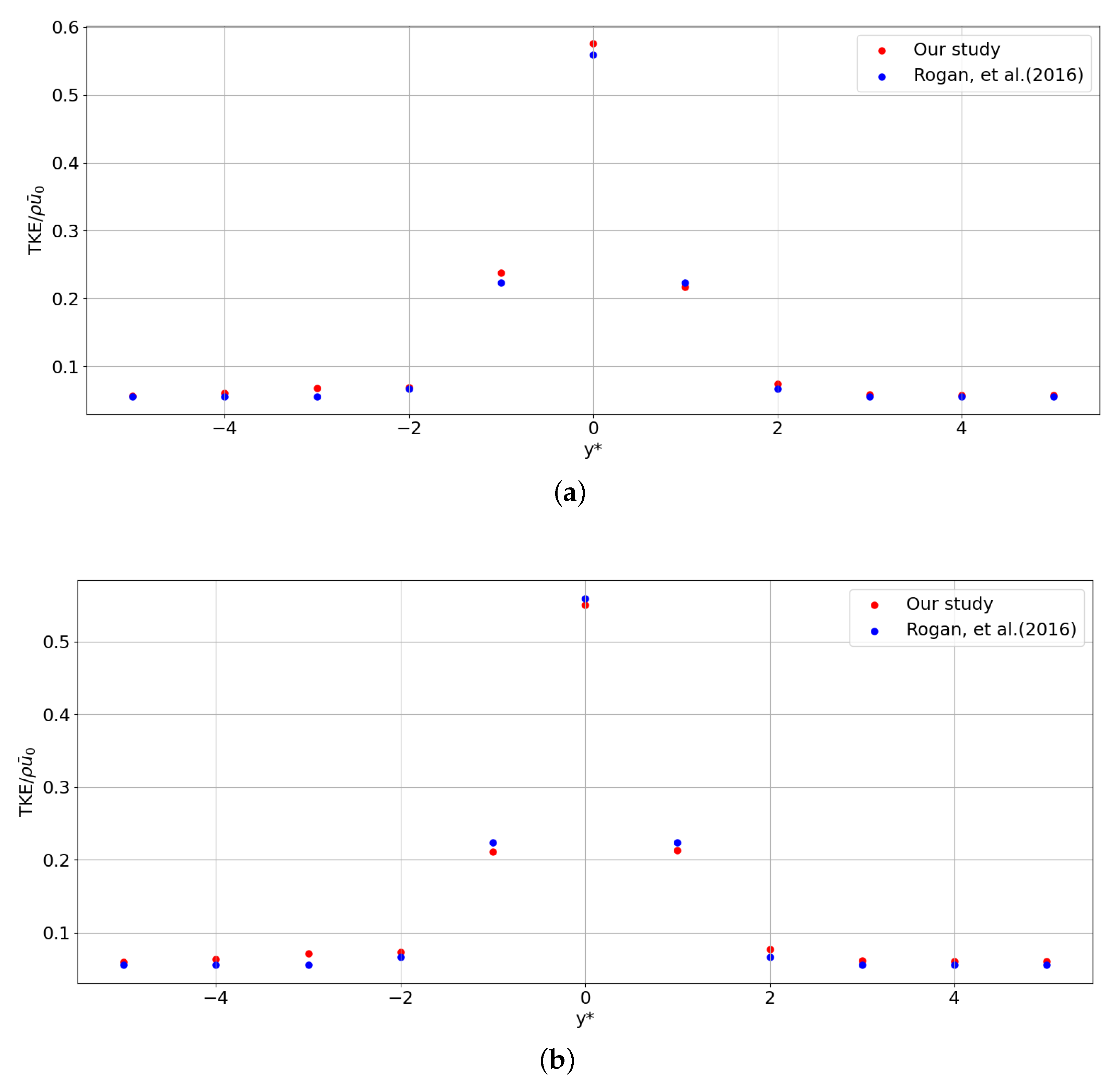
3.3. Results
4. A Real Test Case
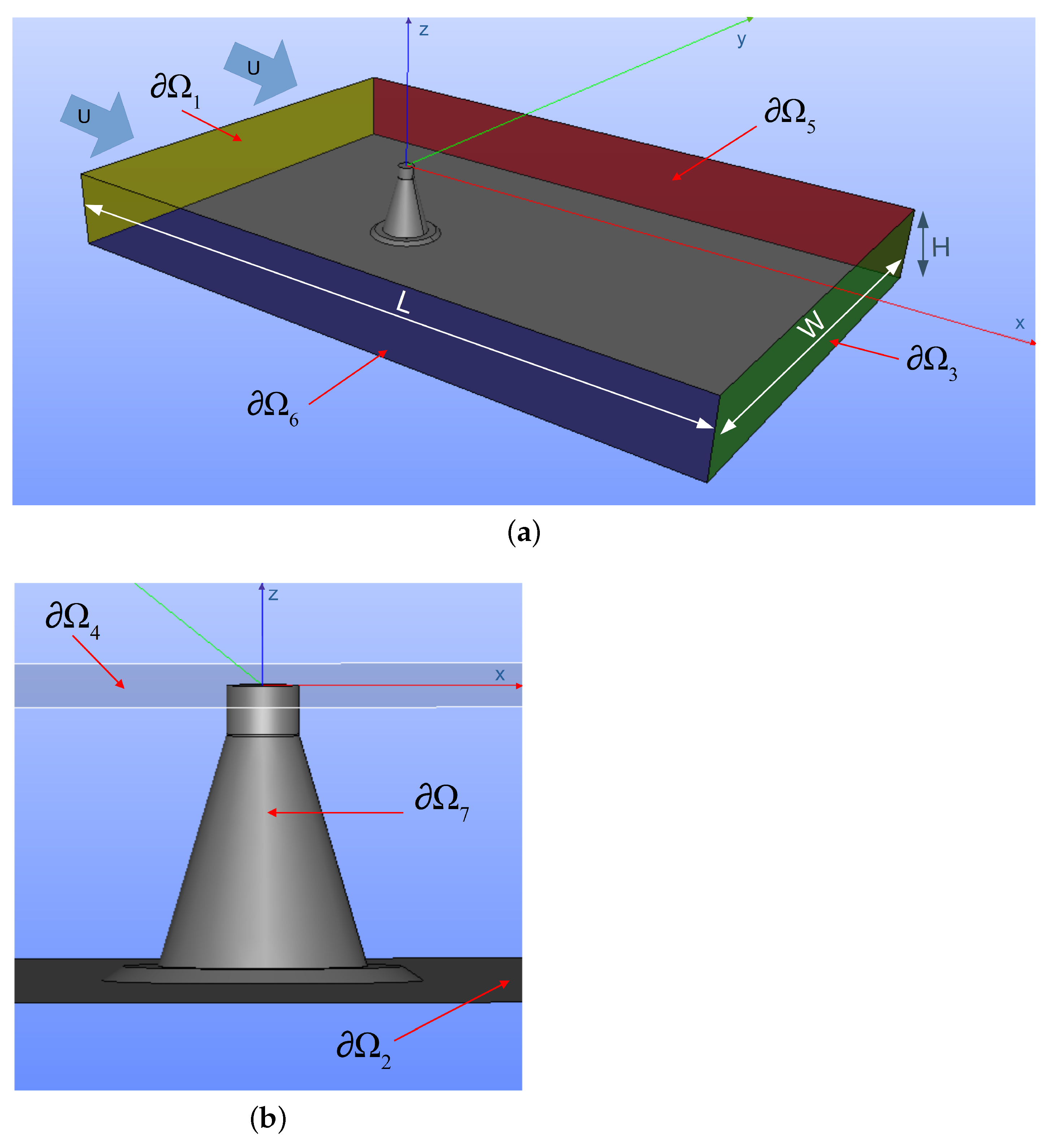
4.1. Domain Geometry
4.2. Mesh
4.3. Larvae Dispersion Simulations
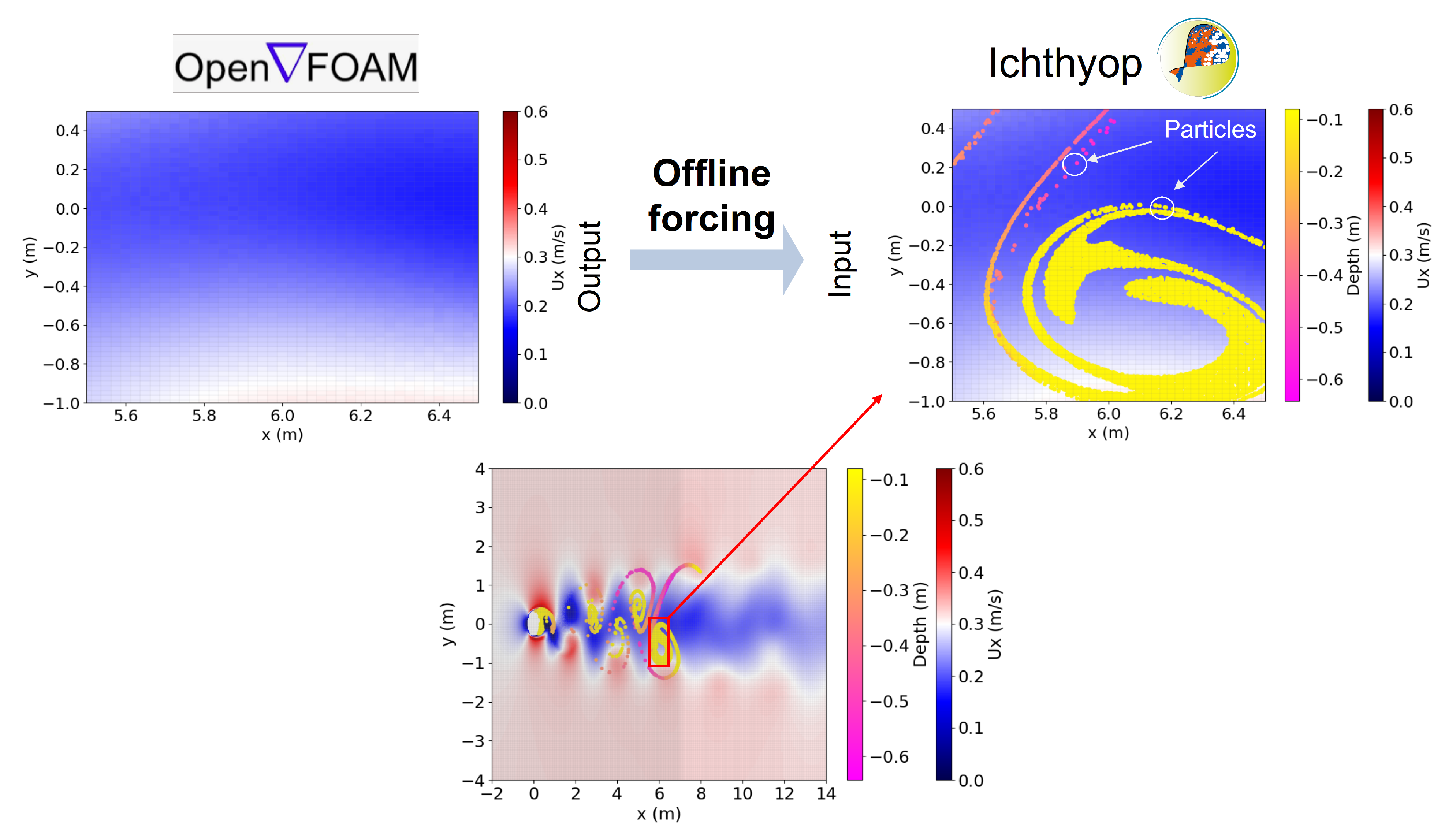
4.4. Coupling Procedure
4.5. Results
4.5.1. General Hydrodynamics
4.5.2. Sensitivity Tests
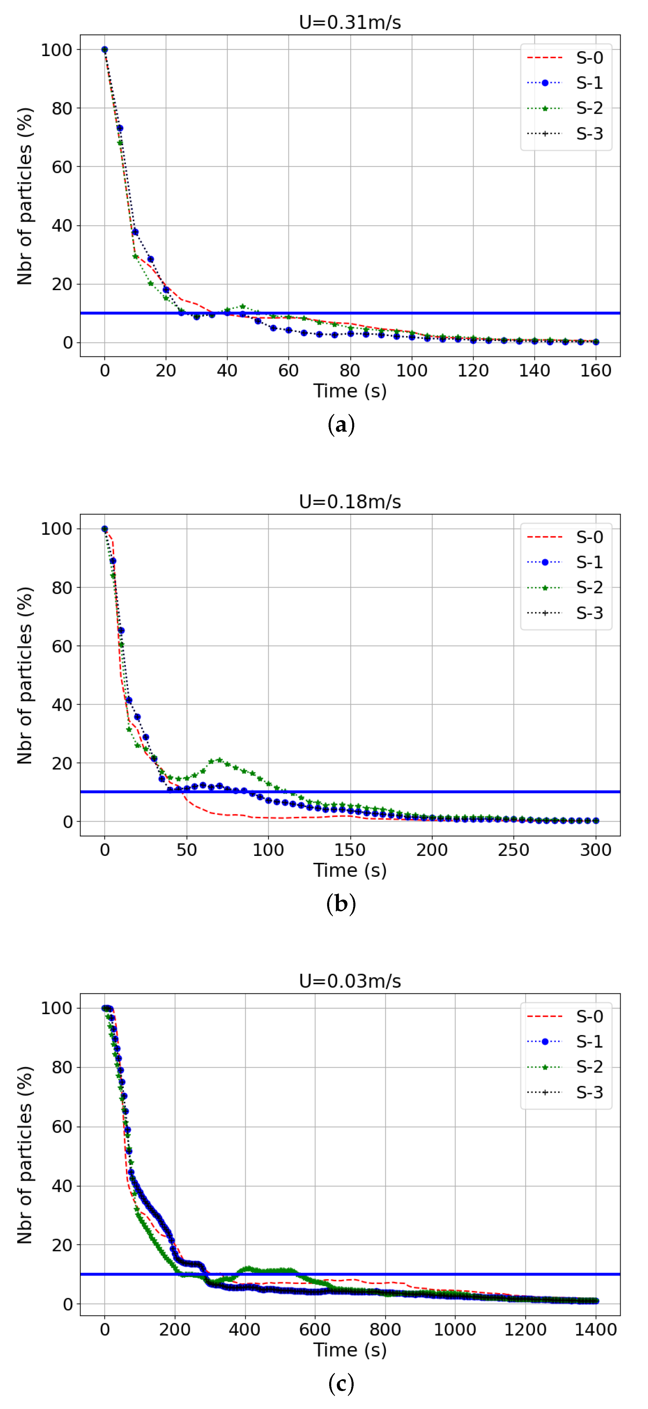
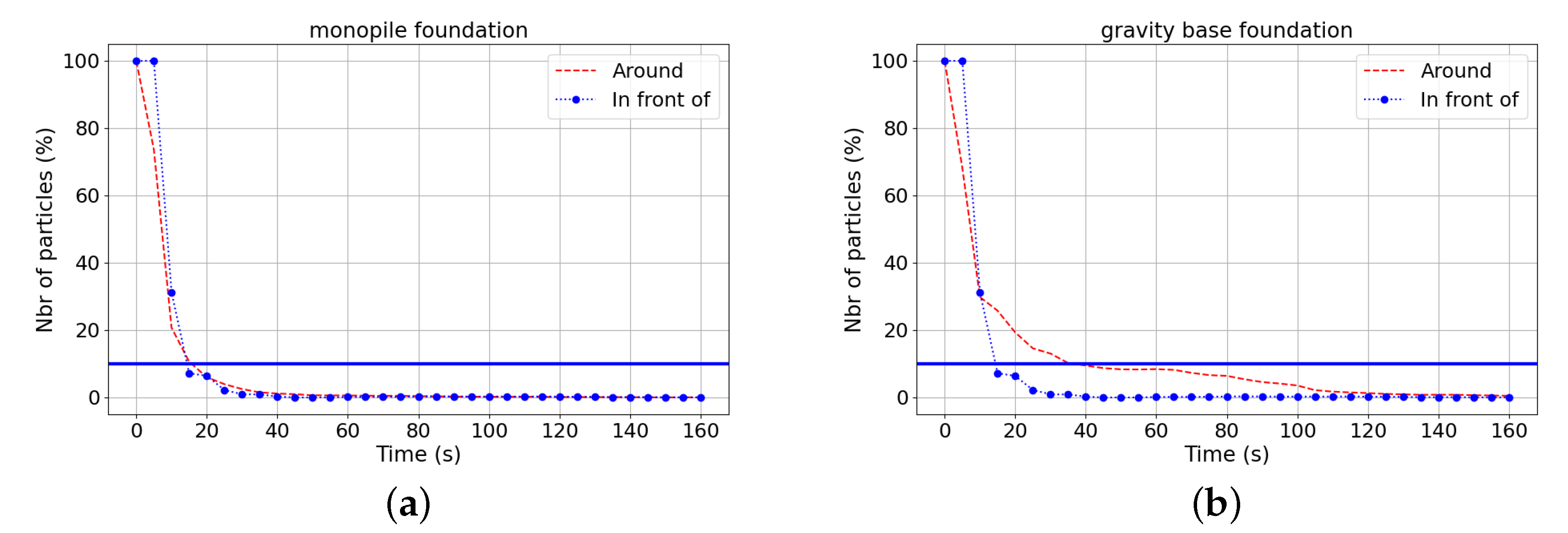
- Effects of the Magnitude of Input VelocityUsing several input velocity values resulted in different retention times for particles to spread in three-dimensional space. To evaluate the sensitivity to the velocity value and initial release depth on larval dispersal, the retention time was found versus the percentage of particles that remained inside the retention box () around the foundations (see Figure 16b). The same size for the retention boxes was chosen for the monopile and gravity-based foundations. For each test, a retention time was calculated, which represents the period of time that the particles have remained close to the foundation inside the retention box until having of the particles. As observed in Figure 20 and Figure 21, the particle retention over time was slightly higher for the gravity-based structure than for the monopile foundation for every inlet velocity and depth release (see Table 6 and Table 7). The longest retention time obtained for one foundation was about . This time was still much lower than the required time to have a real settlement around the structures. To add to this, the larval phase was between 3 weeks to 2 months for our study case, which took into account four benthic species (mussels, oysters, edible crabs, and Asian shore crabs) living in the Bay of Seine [54,55,56,57]. Hence, the longest retention time with U and a release at below the water surface could be possible if considering particles coming from outside of the OWF and having already the competence to settle, depending the species.
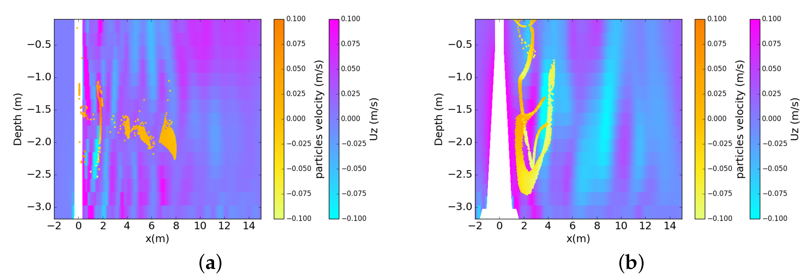
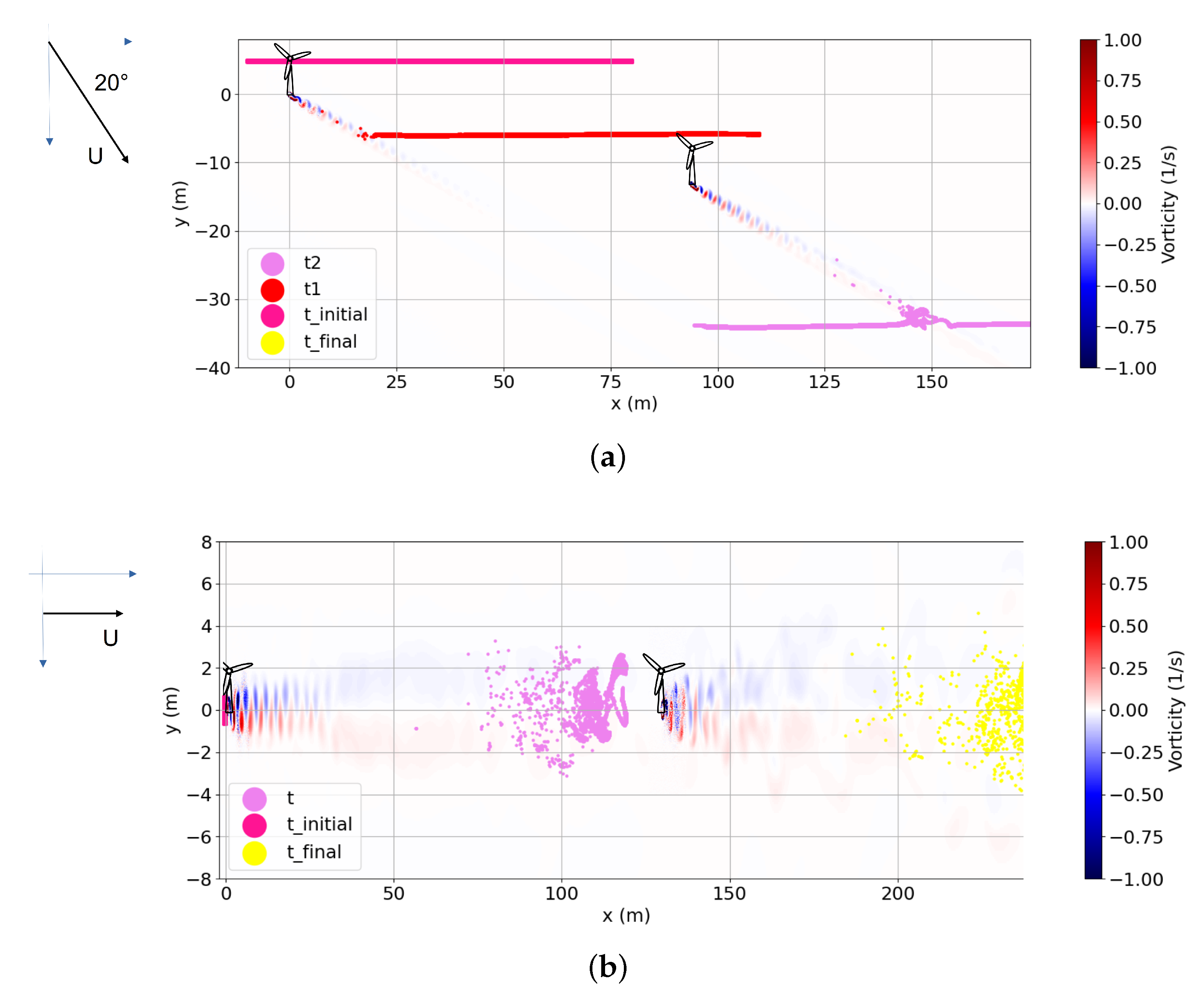
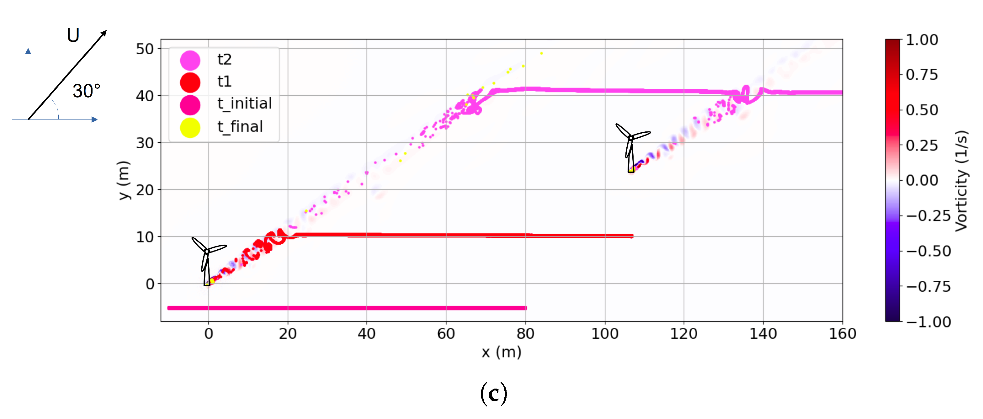
- Influence of the Type of FoundationsThe structure–flow interaction generated a rhythmic flow past a circular cylinder, which can be affected by the vertical shape of the structure. In Figure 22, the vertical velocity related to the wake vortices is shown in the case of a release at below the surface and for a uniform inlet velocity equal to .The vertical flow of wake vortices, as described by [9], drives the particle motions. The larval passive vertical velocity ultimately reflects a fluid force acting on the body motions. For a gravity-based foundation, particles had a faster vertical movement, probably the result of the conical large base (Figure 22) compared to a monopile foundation. To assess differences between the monopile and gravity-based foundations, a retention time was calculated for the gravity-based foundation for different initial depth releases around the structure and for several velocity values (see Table 6 and Table 7). The intense vertical flow generated by the gravity-based foundation led to an increase in the retention time until 9 min against 4 min for a monopile foundation in the case of an input velocity of U (see Table 8) and a release near the bottom (at below the water surface). There were no more larvae after 21 min in the retention box.
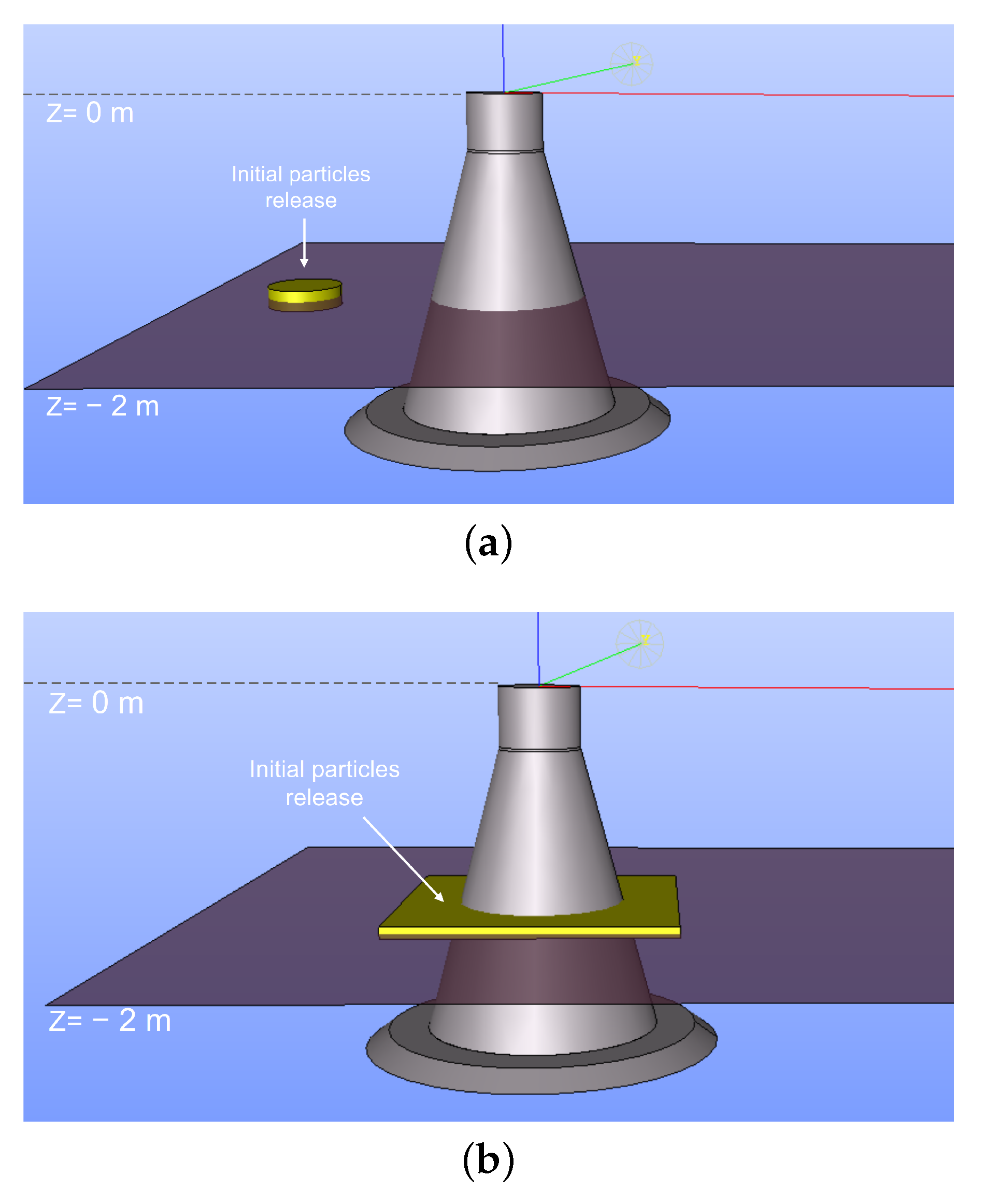
- Impact of the Type of ReleaseThis was almost similar in terms of the retention time versus the percentage of particles in the case of the monopile foundation, and a slight difference was observed in the case of the gravity-based foundation (see Figure 23). During the dispersion, there was a greater number of particles in the case where the initial release was behind the structure and for the gravity-based foundation. This result could be caused by the distance that the geometry of the structure took.
4.6. Case of an Array of Foundations
4.7. Assessment of a Possible Reef Effect or Stepping-Stone Effects
5. Conclusions
Author Contributions
Funding
Institutional Review Board Statement
Informed Consent Statement
Data Availability Statement
Acknowledgments
Conflicts of Interest
References
- Aminoroayaie Yamini, O.; Mousavi, S.H.; Kavianpour, M.R.; Movahedi, A. Numerical modelling of sediment scouring phenomenon around the offshore wind turbine pile in marine environment. Environ. Earth Sci. 2018, 77, 776. [Google Scholar] [CrossRef]
- Díaz, H.; Soares, C.G. Review of the current status, technology and future trends of offshore wind farms. Ocean Eng. 2020, 209, 107381. [Google Scholar] [CrossRef]
- Sánchez, S.; López-Gutiérrez, J.S.; Negro, V.; Esteban, M.D. Foundations in offshore wind farms: Evolution, characteristics and range of use. Analysis of main dimensional parameters in monopile foundations. J. Mar. Sci. Eng. 2019, 7, 441. [Google Scholar] [CrossRef]
- Lavanya, C.; Kumar, N.D. Foundation Types for Land and Offshore Sustainable Wind Energy Turbine Towers. E3S Web Conf. 2020, 184, 01094. [Google Scholar] [CrossRef]
- Rivier, A.; Bennis, A.C.; Pinon, G.; Magar, V.; Gross, M. Parameterization of wind turbine impacts on hydrodynamics and sediment transport. Ocean Dyn. 2016, 66, 1285–1299. [Google Scholar] [CrossRef]
- Pezy, J.P.; Dauvin, J.C. Wide coverage but few quantitative data: Coarse sediments in the English Channel. Ecol. Indic. 2021, 121, 107010. [Google Scholar] [CrossRef]
- Méar, Y.; Poizot, E.; Murat, A.; Beryouni, K.; Baux, N.; Dauvin, J.C. Improving the monitoring of a dumping site in a dynamic environment. Example of the Octeville site (Bay of Seine, English Channel). Mar. Pollut. Bull. 2018, 129, 425–437. [Google Scholar] [CrossRef]
- Clark, S.; Schroeder, F.; Baschek, B. The Influence of Large Offshore Wind Farms on the North Sea and Baltic Sea: A Comprehensive Literature Review; Helmholtz-Zentrum Geesthacht, Zentrum für Material-und Küstenforschung: Geesthacht, Germany, 2014. [Google Scholar]
- Petersen, T.U.; Sumer, B.M.; Fredsøe, J.; Raaijmakers, T.C.; Schouten, J.J. Edge scour at scour protections around piles in the marine environment—Laboratory and field investigation. Coast. Eng. 2015, 106, 42–72. [Google Scholar] [CrossRef]
- Christensen, E.D.; Johnson, M.; Sørensen, O.R.; Hasager, C.B.; Badger, M.; Larsen, S.E. Transmission of wave energy through an offshore wind turbine farm. Coast. Eng. 2013, 82, 25–46. [Google Scholar] [CrossRef]
- Wieselsberger, C. New data on the laws of fluid resistance. Phys. Z. 1922, 22, 321–328. [Google Scholar]
- Thom, A. The flow past circular cylinders at low speeds. Proc. R. Soc. Lond. A 1933, 141, 651–669. [Google Scholar]
- Homann, F. Einfluß großer zähigkeit bei strömung um zylinder. Forschung auf dem Gebiet des Ingenieurwesens A 1936, 7, 1–10. [Google Scholar] [CrossRef]
- Sarpkaya, T. Vortex Shedding and Resistance in Harmonic Flow about Smooth and Rough Circular Cylinders at High Reynolds Numbers; Technical Report; Naval Postgraduate School: Monterey, CA, USA, 1976. [Google Scholar]
- Kawamura, T.; Hiwada, M.; Hibino, T.; Mabuchi, I.; Kumada, M. Flow around a finite circular cylinder on a flat plate: Cylinder height greater than turbulent boundary layer thickness. Bull. JSME 1984, 27, 2142–2151. [Google Scholar] [CrossRef]
- Eckerle, W.A.; Langston, L. Horseshoe vortex formation around a cylinder. J. Turbomach. 1987, 109, 278–285. [Google Scholar] [CrossRef]
- Sumer, B.M.; Fredsøe, J. Scour at the head of a vertical-wall breakwater. Coast. Eng. 1997, 29, 201–230. [Google Scholar] [CrossRef]
- Williamson, C. Three-dimensional wake transition. J. Fluid Mech. 1996, 328, 345–407. [Google Scholar] [CrossRef]
- Fredsoe, J.; Sumer, B.M. Hydrodynamics around Cylindrical Structures, Revised ed.; World Scientific Publishing Company: Singapore, 2006; Volume 26. [Google Scholar]
- Zhang, H.Q.; Fey, U.; Noack, B.R.; König, M.; Eckelmann, H. On the transition of the cylinder wake. Phys. Fluids 1995, 7, 779–794. [Google Scholar] [CrossRef]
- Orszag, S.A. Analytical theories of turbulence. J. Fluid Mech. 1970, 41, 363–386. [Google Scholar] [CrossRef]
- Wilcox, D.C. Reassessment of the scale-determining equation for advanced turbulence models. AIAA J. 1988, 26, 1299–1310. [Google Scholar] [CrossRef]
- Menter, F.R. Two-equation eddy-viscosity turbulence models for engineering applications. AIAA J. 1994, 32, 1598–1605. [Google Scholar] [CrossRef]
- Celik, I.; Shaffer, F.D. Long time-averaged solutions of turbulent flow past a circular cylinder. J. Wind Eng. Ind. Aerodyn. 1995, 56, 185–212. [Google Scholar] [CrossRef]
- Khan, N.B.; Ibrahim, Z. Numerical investigation of vortex-induced vibration of an elastically mounted circular cylinder with One-degree of freedom at high Reynolds number using different turbulent models. Proc. Inst. Mech. Eng. Part M J. Eng. Marit. Environ. 2019, 233, 443–453. [Google Scholar] [CrossRef]
- Planes, S.; Parroni, M.; Chauvet, C. Evidence of limited gene flow in three species of coral reef fishes in the lagoon of New Caledonia. Mar. Biol. 1998, 130, 361–368. [Google Scholar] [CrossRef]
- Dannheim, J.; Bergström, L.; Birchenough, S.N.; Brzana, R.; Boon, A.R.; Coolen, J.W.; Dauvin, J.C.; De Mesel, I.; Derweduwen, J.; Gill, A.B.; et al. Benthic effects of offshore renewables: Identification of knowledge gaps and urgently needed research. ICES J. Mar. Sci. 2020, 77, 1092–1108. [Google Scholar] [CrossRef]
- Van Berkel, J.; Burchard, H.; Christensen, A.; Mortensen, L.O.; Petersen, O.S.; Thomsen, F. The effects of offshore wind farms on hydrodynamics and implications for fishes. Oceanography 2020, 33, 108–117. [Google Scholar] [CrossRef]
- Nicolle, A.; Dumas, F.; Foveau, A.; Foucher, E.; Thiébaut, E. Modelling larval dispersal of the king scallop (Pecten maximus) in the English Channel: Examples from the bay of Saint-Brieuc and the bay of Seine. Ocean. Dyn. 2013, 63, 661–678. [Google Scholar] [CrossRef]
- Adams, T.P.; Miller, R.G.; Aleynik, D.; Burrows, M.T. Offshore marine renewable energy devices as stepping stones across biogeographical boundaries. J. Appl. Ecol. 2014, 51, 330–338. [Google Scholar] [CrossRef]
- Greifzu, F.; Kratzsch, C.; Forgber, T.; Lindner, F.; Schwarze, R. Assessment of particle-tracking models for dispersed particle-laden flows implemented in OpenFOAM and ANSYS FLUENT. Eng. Appl. Comput. Fluid Mech. 2016, 10, 30–43. [Google Scholar] [CrossRef]
- Floeter, J.; van Beusekom, J.E.; Auch, D.; Callies, U.; Carpenter, J.; Dudeck, T.; Eberle, S.; Eckhardt, A.; Gloe, D.; Hänselmann, K.; et al. Pelagic effects of offshore wind farm foundations in the stratified North Sea. Prog. Oceanogr. 2017, 156, 154–173. [Google Scholar] [CrossRef]
- Pothin, K. Analyse de la Dispersion Larvaire des Poissons Récifaux à la Réunion à Travers l’étude de Leurs Otolithes. Ph.D. Thesis, Université de La Réunion, Saint-Denis, France, 2005. [Google Scholar]
- Esteban, M.D.; López-Gutiérrez, J.S.; Negro, V. Gravity-based foundations in the offshore wind sector. J. Mar. Sci. Eng. 2019, 7, 64. [Google Scholar] [CrossRef]
- Wu, X.; Hu, Y.; Li, Y.; Yang, J.; Duan, L.; Wang, T.; Adcock, T.; Jiang, Z.; Gao, Z.; Lin, Z.; et al. Foundations of offshore wind turbines: A review. Renew. Sustain. Energy Rev. 2019, 104, 379–393. [Google Scholar] [CrossRef]
- Rogan, C.; Miles, J.; Simmonds, D.; Iglesias, G. The turbulent wake of a monopile foundation. Renew. Energy 2016, 93, 180–187. [Google Scholar] [CrossRef]
- Greenshields; Christopher. OpenFOAM User Guide; OpenFOAM Found. Ltd Version; The OpenFOAM Foundation: London, UK, 2015; Volume 3, p. 47. [Google Scholar]
- Issa, R.I. Solution of the implicitly discretised fluid flow equations by operator-splitting. J. Comput. Phys. 1986, 62, 40–65. [Google Scholar] [CrossRef]
- Patankar, S.V.; Spalding, D.B. A calculation procedure for heat, mass and momentum transfer in three-dimensional parabolic flows. Int. J. Heat Mass Transf. 1983, 1, 54–73. [Google Scholar]
- Aravind Karthik, M.; Srinivas, G.; Naik, N. Implementation of Higher-Order PIMPLE Algorithm for Time Marching Analysis of Transonic Wing Compressibility Effects with High Mach Pre-Conditioning. Eng. Sci. 2022, 20, 218–235. [Google Scholar]
- Liu, Y.; Xiao, Q.; Incecik, A.; Peyrard, C.; Wan, D. Establishing a fully coupled CFD analysis tool for floating offshore wind turbines. Renew. Energy 2017, 112, 280–301. [Google Scholar] [CrossRef]
- Wilcox, D.; Traci, R. A complete model of turbulence. In Proceedings of the 9th Fluid and PlasmaDynamics Conference, San Diego, CA, USA, 14–16 July 1976; p. 351. [Google Scholar]
- Courant, R.; Friedrichs, K.; Lewy, H. Uber die Differenzengleichungen der Mathematischen Physik. Math. Ann. 1928, 100, 32. [Google Scholar] [CrossRef]
- Gy, P. Sampling for Analytical Purposes; John Wiley & Sons: Hoboken, NJ, USA, 1998. [Google Scholar]
- Manual, U. ANSYS FLUENT 12.0; Theory Guide; ANSYS Inc.: Cannonsburg, PA, USA, 2009; Available online: https://www.afs.enea.it/project/neptunius/docs/fluent/html/th/main_pre.htm (accessed on 7 November 2023).
- Lett, C.; Verley, P.; Mullon, C.; Parada, C.; Brochier, T.; Penven, P.; Blanke, B. A Lagrangian tool for modelling ichthyoplankton dynamics. Environ. Model. Softw. 2008, 23, 1210–1214. [Google Scholar] [CrossRef]
- Davidson, F.J.; Deyoung, B. Modelling advection of cod eggs and larvae on the Newfoundland Shelf. Fish. Oceanogr. 1995, 4, 33–51. [Google Scholar] [CrossRef]
- Collins, C.; Hermes, J. Modelling the accumulation and transport of floating marine micro-plastics around South Africa. Mar. Pollut. Bull. 2019, 139, 46–58. [Google Scholar] [CrossRef]
- Peliz, A.; Marchesiello, P.; Dubert, J.; Marta-Almeida, M.; Roy, C.; Queiroga, H. A study of crab larvae dispersal on the Western Iberian Shelf: Physical processes. J. Mar. Syst. 2007, 68, 215–236. [Google Scholar] [CrossRef]
- Norberg, C. Effects of Reynolds Number and a Low-Intensity Freestream Turbulence on the Flow around a Circular Cylinder; Chalmers University of Technology: Gothenburg, Sweden, 1987; Volume 87, pp. 1–55. [Google Scholar]
- Ajmi, S.; Boutet, M.; Bennis, A.C.; Pezy, J.P.; Dauvin, J.C. Impact of the turbulent wake downstream offshore wind turbines on larval dispersal. Trends Renew. Energ. Offshore 2022, 10, 3–8. [Google Scholar]
- Strouhal, V. Über eine besondere Art der Tonerregung. Ann. Phys. 1878, 24, 216251. [Google Scholar]
- Blevins, R.D. Flow-Induced Vibration; Van Nostrand Reinhold Company: New York, NY, USA, 1977. [Google Scholar]
- Toupoint, N.; Mohit, V.; Linossier, I.; Bourgougnon, N.; Myrand, B.; Olivier, F.; Lovejoy, C.; Tremblay, R. Effect of biofilm age on settlement of Mytilus edulis. Biofouling 2012, 28, 985–1001. [Google Scholar] [CrossRef]
- His, E.; Robert, R. Developpement des veligeres de Crassostrea gigas dans le bassin d’Arcachon. Etudes sur les mortalites larvaires. Rev. Trav. De l’Institut Pêches Marit. 1983, 47, 63–88. [Google Scholar]
- Bennett, D.B. Factors in the life history of the edible crab (Cancer pagurus L.) that influence modelling and management. Ices Mar. Sci. Symp. 1995, 199, 89–98. [Google Scholar]
- Epifanio, C.E. Invasion biology of the Asian shore crab Hemigrapsus sanguineus: A review. J. Exp. Mar. Biol. Ecol. 2013, 441, 33–49. [Google Scholar] [CrossRef]
- Butman, C. Larval settlement of soft-sediment invertebrates: The spatial scales of pattern explained by active habitat selection and the emerging role of hydrodynamical processes. Oceanogr. Mar. Biol. 1987, 25, 113–165. [Google Scholar]


| Monopile | |
|---|---|
| Minimum cell volume () | |
| Maximum cell volume () | |
| Cell number | 7,775,424 |
| Point number | 8,043,111 |
| 1 Foundation | 2 Foundations | |||
|---|---|---|---|---|
| Monopile | Gravity-Based | Monopile | Gravity-Based | |
| Minimum cell volume () | ||||
| Maximum cell volume () | ||||
| Cell number | ||||
| Point number | ||||
| Level 1 | Level 2 | |
|---|---|---|
| Minimum cell volume () | ||
| Maximum cell volume () | ||
| Cell number | ||
| Point number |
| f | |||
| f (Hz) | |||
| 16 s | 30 s | 200 s | |
| 17 s | 33 s | 200 s | |
| 19 s | 40 s | 240 s | |
| 18 s | 33 s | 220 s |
| 40 s | 45 s | 335 s | |
| 45 s | 80 s | 290 s | |
| 55 s | 115 s | 540 s | |
| 45 s | 80 s | 290 s |
| Monopile | Gravity-Based | |||
|---|---|---|---|---|
| In Front of | Around | In Front of | Around | |
| 14 s | 15 s | 14 s | 40 s | |
| 190 s | 200 s | 480 s | 335 s | |
| No. of Settled Particles (%) | |
|---|---|
| Monopile ( ) | 0 |
| Monopile ( ) | 0 |
| Gravity-based ( ) |
Disclaimer/Publisher’s Note: The statements, opinions and data contained in all publications are solely those of the individual author(s) and contributor(s) and not of MDPI and/or the editor(s). MDPI and/or the editor(s) disclaim responsibility for any injury to people or property resulting from any ideas, methods, instructions or products referred to in the content. |
© 2023 by the authors. Licensee MDPI, Basel, Switzerland. This article is an open access article distributed under the terms and conditions of the Creative Commons Attribution (CC BY) license (https://creativecommons.org/licenses/by/4.0/).
Share and Cite
Ajmi, S.; Boutet, M.; Bennis, A.-C.; Dauvin, J.-C.; Pezy, J.-P. Numerical Study of Turbulent Wake of Offshore Wind Turbines and Retention Time of Larval Dispersion. J. Mar. Sci. Eng. 2023, 11, 2152. https://doi.org/10.3390/jmse11112152
Ajmi S, Boutet M, Bennis A-C, Dauvin J-C, Pezy J-P. Numerical Study of Turbulent Wake of Offshore Wind Turbines and Retention Time of Larval Dispersion. Journal of Marine Science and Engineering. 2023; 11(11):2152. https://doi.org/10.3390/jmse11112152
Chicago/Turabian StyleAjmi, Souha, Martial Boutet, Anne-Claire Bennis, Jean-Claude Dauvin, and Jean-Philippe Pezy. 2023. "Numerical Study of Turbulent Wake of Offshore Wind Turbines and Retention Time of Larval Dispersion" Journal of Marine Science and Engineering 11, no. 11: 2152. https://doi.org/10.3390/jmse11112152
APA StyleAjmi, S., Boutet, M., Bennis, A.-C., Dauvin, J.-C., & Pezy, J.-P. (2023). Numerical Study of Turbulent Wake of Offshore Wind Turbines and Retention Time of Larval Dispersion. Journal of Marine Science and Engineering, 11(11), 2152. https://doi.org/10.3390/jmse11112152