Multivariate Sea Surface Prediction in the Bohai Sea Using a Data-Driven Model

Abstract

Data-driven predictions of marine environmental variables are typically focused on single variables. However, in real marine environments, there are correlations among different oceanic variables. Additionally, sea–air interactions play a significant role in influencing the evolution of the marine environment. Both internal dynamics and external drivers contribute to these changes. In this study, a data-driven model is proposed using sea surface height anomaly (SSHA), sea surface temperature (SST), and sea surface wind (SSW) in the Bohai Sea. This model combines multivariate empirical orthogonal functions (MEOFs) with long and short-term memory (LSTM). MEOF analysis is used on the multivariate dataset of SSHA and SST, considering the correlation among sea surface variables. SSW is introduced as a predictor to enhance the predictability of the multivariate sea surface model. In the case of the Bohai Sea, the comparative tests of the model without wind field effect, the fully coupled model, and the proposed prediction model were carried out. MEOF analysis is employed in comparative experiments for oceanic variables, atmospheric variables, and combined atmospheric and oceanic variables. The results demonstrate that using wind field as a predictor can improve the forecast accuracy of SSHA and SST in the Bohai Sea. The root mean square errors (RMSE) for SSHA and SST in a 7-day forecast are 0.016 m and 0.3200 °C, respectively.

1. Introduction

Changes in SSHA and SST may lead to some climate extremes [1,2]. Therefore, accurate prediction of SSHA and SST is of great scientific significance [3]. Traditional oceanic numerical models often rely on complex physical parameters and require significant computational resources, which may limit the accuracy of predictions. However, with the continuous enrichment of ocean data types and volumes, data-driven prediction has gradually become a research hotspot [4,5,6]. Data-driven approaches are primarily based on objective data itself, free from the constraints of physical equations, and they greatly reduce the influence of parameter uncertainties. This allows for more accurate predictions and less reliance on complex physical modeling.

Data-driven methods can effectively use historical data to extract valuable information from them and make forecasts. There are two primary classifications of data-driven forecasting techniques: conventional statistical forecasting techniques and neural network prediction methods. Common statistical forecasting techniques include empirical orthogonal function (EOF) decomposition [7], multivariate empirical orthogonal functions (MEOF) decomposition [8], linear regression (LR) techniques [9,10], conventional correlation analysis methods [11], and support vector machines (SVM) [12,13]. Neural network prediction methods encompass various types, including artificial neural networks (ANNs) [14,15], gated recurrent unit (GRU) neural network [16], memory in memory (MIM) neural network [17], deep neural networks (DNNs) [18], LSTM network [19,20,21], and back propagation (BP) neural networks [22]. Additionally, there is the transfer learning model [23].

Recent studies have utilized data-driven approaches to predict various oceanic variables. For example, Zhang et al. used a long-short memory (LSTM) network to predict the SST in the Bohai Sea [24]; Wei et al. used a multilayer perceptron (MLP) model to predict the SST in the South China Sea [25]; Xie et al. combined deep learning with the attention mechanism to construct an adaptive model for SST prediction in the Bohai Sea region [26]; Xie et al. proposed a method to predict the SST in the Bohai Sea by combining the convolutional gated recurrent unit (GRU) and the multilayer perceptron (CGMP) [27]; Zhang et al. developed a model based on gated recurrent unit (GRU) neural networks to predict SST over the medium- and long-term and used multiple time-scale datasets; researchers conducted experiments in the Bohai Sea [28]; Gao et al. proposed a global spatio-temporal graph attention network (GSTGAT) in combination with a graph neural network (GNN); and multiple time-scale datasets in the Bohai Sea were used to conduct experiments [29].

However, most of the above studies construct prediction models for single variables under single scale conditions and ignore the influence of external drivers. This may limit the improving of forecasting accuracy. To enhance the consistency between data-driven models and actual physical variation processes, it is important to consider the correlation between different ocean variables. In this study, we adopt a similar data-driven forecasting framework as previous studies [30,31,32,33]. However, it is worth noting that our previous study is based on the South China Sea (SCS) region with a mean water depth of 1200 m. In this region, the internal dynamical mechanisms dominate the oceanic evolution process, and the influence of external drivers is relatively small. Hence, the combined forecasting technique for oceanic variables proves to be efficient in the South China Sea. Regarding the study area of this study, which is the Bohai Sea, it has an average depth of only 18 m. In the oceanic evolution process of the Bohai Sea, meteorological driving factors and internal dynamic mechanisms have comparable roles. Thus, it is necessary to introduce external drivers into the coupled model and examine the results obtained through different coupling methods. In addition, the interaction between the atmosphere and the ocean drives us to think about how to introduce atmospheric information into the data-driven models.

A data-driven forecasting model for SSHA and SST in the Bohai Sea is constructed by using MEOF analysis and an LSTM neural network. In particular, the sea surface wind field is introduced into the model as a predictor to improve the forecast accuracy. This method not only considers the dynamical coordination relationship between different variables in the ocean but also takes into account the role of the atmosphere on the ocean, which can improve the forecast accuracy of marine environmental variables.

The remaining portion of this document is structured in the following manner: Section 2 provides an explanation of the data and methodologies employed in this research. In Section 3, the model prediction experiments and results for SSHA and SST in the Bohai Sea are presented. Finally, Section 4 gives the conclusions.

2. Data and Methodology

2.1. Study Area and Data Collection

In this study, the proposed model performance is assessed by analyzing long-term satellite remote sensing data for SSHA, SST, and SSW (U and V component) within the geographical coordinates of 116° to 124° E and 36° to 42° N, specifically in the Bohai Sea of China. SSHA and SST are two important variables in the ocean environment that can directly reflect the changes generated by the ocean. SSW is one of the ways for the exchange of heat between the ocean and the atmosphere and acts as a medium for their interaction. In the subsequent construction of the prediction model, SSW represents an external driver, enabling the model to better simulate real evolution in the ocean environment.

The SSHA here are daily 1/4° data provided by Copernicus Marine and Environmental Monitoring Service (CMEMS). The SST data used are the 1/4° daily best interpolated sea surface temperature (OISST) from National Oceanic and Atmospheric Administration (NOAA). The SSW (U and V component) is the Cross-Calibrated Multi-Platform (CCMP) wind field, which is obtained from NASA Earth Science Enterprise (ESE). The data used in this study span a time length of 28 years, from January 1993 to December 2020. The training dataset includes data from 1993 to 2015, while the model validation adopts independent experimental samples from 2016 to 2020, with a time span of 5 years.

2.2. Proposed Model

This study presents a forecasting model for predicting SSHA and SST in the Bohai Sea, utilizing MEOF analysis and an LSTM neural network. Figure 1 provides a visual representation of the model, highlighting its three primary components: the MEOF analysis phase, the LSTM neural network prediction phase, and the data reconstruction phase.

In the stage of MEOF analysis, the preprocessed satellite data variables are separated into a training set and a testing set. The orthogonal spatial patterns and principal components (PCs) of the training set are obtained by MEOF decomposition. The orthogonal spatial patterns are called EOFs. The PCs of the testing set can be obtained by projecting onto the EOFs. Section 2.3 summarizes the MEOF analysis process.

In the prediction stage of the LSTM neural network, PCs with a certain variance ratio are selected from the previous step and used as the input of the LSTM neural network. The predictive value of PCs is obtained by using an LSTM neural network. Section 2.4 describes the LSTM network used in this study.

During the data reconstruction stage, the reconstructed field is achieved by combining the prediction values of the PCs with the EOFs.

2.3. MEOF Analysis

MEOF analysis is a valuable tool for examining the spatial and temporal distribution characteristics of variables within the ocean and atmospheric domains. In this study, MEOF analysis is adopted to decompose the multivariate sample matrix composed of SSHA and SST. The U and V components of SSW (referred to as Uwind and Vwind) are also subjected to the same decomposition. Additionally, the MEOF analysis is employed to decompose the multivariate sample matrix consisting of SSHA, SST, Uwind, and Vwind. The specific expressions are as follows.

$$X_1=\left[\begin{array}{ccccc}{X}_{SSHA}^1& \cdots & X_{SSHA}^m& \cdots & X_{SSHA}^M\\ X_{SST}^1& \cdots & X_{SST}^m& \cdots & X_{SST}^M\end{array}\right]$$

(1)

$$X_2=\left[\begin{array}{ccccc}{X}_{Uwind}^1& \cdots & X_{Uwind}^m& \cdots & X_{Uwind}^M\\ X_{Vwind}^1& \cdots & X_{Vwind}^m& \cdots & X_{Vwind}^M\end{array}\right]$$

(2)

$$X_3=\left[\begin{array}{ccccc}{X}_{SSHA}^1& \cdots & X_{SSHA}^m& \cdots & X_{SSHA}^M\\ X_{SST}^1& \cdots & X_{SST}^m& \cdots & X_{SST}^M\\ X_{Uwind}^1& \cdots & X_{Uwind}^m& \cdots & X_{Uwind}^M\\ X_{Vwind}^1& \cdots & X_{Vwind}^m& \cdots & X_{Vwind}^M\end{array}\right]$$

(3)

where $X_{SSHA}^m$ is the SSHA sample on the $mth$ day. SST, Uwind, and Vwind are expressed in the same way. The spatial dimension of each variable is denoted by $N$. The time dimension of each variable is represented by $M$. The spatial dimension of the four variables is uniform, so the dimension of each sample matrix is $N\times M$. In this study, $N$ and $M$ are 257 points and 8395 days, respectively.

In this study, we are more concerned with the variation of the anomalies of variables, which are constructed by subtracting the climatology.

$$X_1^{\prime }=X_1-{\overline{X}}_1$$

(4)

where $X_1^{\prime }$ denotes the anomaly sample matrix, and ${\overline{X}}_1$ denotes the climatology mean.

The covariance matrix $C_{2N\times 2N}$ of matrix $X_1^{\prime }$ can be expressed as follows:

$$C_{2N\times 2N}=\frac{1}{M}{X}_1^{\prime }\times X_1^{\prime T}$$

(5)

It is important to mention that $C_{2N\times 2N}$ effectively takes into account the relationship between various variables. Expression of eigenvalues and eigenvectors as:

$$C_{2N\times 2N}\times V_{2N\times 2N}=V_{2N\times 2N}\times E_{2N\times 2N}$$

(6)

The arrangement of eigenvalues is in descending order. In $E_{2N\times 2N}$, each non-zero eigenvalue corresponds to an eigenvector; $V_{2N\times 2N}$ is also known as orthogonal spatial patterns. The orthogonal spatial patterns are called EOFs. EOFs can be projected onto the total sample matrix to obtain the principal components ($PC$), expressed as:

$$P{C}_{2N\times M}=V_{2N\times 2N}^T\times X_1^{\prime }$$

(7)

This study utilizes a limited quantity of orthogonal spatial patterns exhibiting significant variance to reconstruct the primary attributes of the spatial composition for each component. The data in $P{C}_{2N\times M}$ represent the $PC$ corresponding to each column of eigenvector.

We retained the top 15 EOFs, accounting for 89% of the total variance. Currently, the primary challenge lies in enhancing the analysis and forecasting of these temporal sequences.

2.4. LSTM

In this study, we utilize LSTM networks, which are an improved type of recurrent neural network (RNN). While traditional neural networks are unable to retain information over time, RNNs with a recurrent structure can do so. However, they face the challenge of vanishing gradients when the information is too distant from the current prediction task. This results in the loss of previous information and the inability to handle long-term dependencies. All recurrent neural networks have a chain-like structure consisting of repeating neural network modules. Standard RNNs, such as single-layer RNNs, have a simple repeating module structure, typically a single tanh layer. However, LSTM networks have a special chaining structure that enables information to be looped. By storing both relevant and long-term information, LSTM networks can effectively address the problem of long-term dependencies and predict longer time series [34].

LSTM networks have the ability to store both short and long-term learning information and can selectively add or delete information. This is achieved through the use of gates that carefully regulate the flow of information. Each gate contains a sigmoid neural network layer, which determines the discarding of useless information, and a point multiplication operation. An LSTM network utilizes three gates to safeguard and regulate the cell state, as depicted in Figure 2.

The formula of the forget gate is expressed as Formula (8), the formula of the input gate is expressed as Formulas (9) and (10), the formula of the cell state is expressed as Formula (11), and the formula of the output gate is expressed as Formulas (12) and (13).

$$f_t=\sigma (W_f\cdot \left[h_{t-1},x_t\right]+b_f)$$

(8)

$$i_t=\sigma (W_i\cdot [h_{t-1},x_t]+b_i)$$

(9)

$${\tilde{C}}_t=\tanh (W_C\cdot [h_{t-1},x_t]+b_C)$$

(10)

$$C_t=f_t\ast C_{t-1}+i_t\ast {\tilde{C}}_t$$

(11)

$$o_t=\sigma (W_o\cdot [h_{t-1},x_t]+b_o)$$

(12)

$$h_t=o_t\ast \tanh (C_t)$$

(13)

In these formulas, the forget gate $f_t$ combines the previous hidden layer state value $h_{t-1}$ with the current input $x_t$. Decide to discard the original information through sigmoid function $\sigma$. Input gates $i_t$ and $\tanh$ determine which information to save in $h_{t-1}$ and $x_t$, and obtain the cell state candidate value ${\tilde{C}}_t$. Cell state $C_t$ indicates the state of discarding and storing information. Finally, the output gate combines $\tanh$ to determine which information in $h_{t-1}$, $x_t$, and $C_t$ is output as the hidden layer state value $h_t$ at this time. $W$ and $b$ are weights and deviations.

In this research, the LSTM model consists of multiple layers, comprising a convolutional layer, a pooling layer, a bidirectional LSTM layer, a concatenate layer, three dropout layers, and three dense layers. This research introduces a one-dimensional convolutional layer that enhances the extraction of input data features. The convolutional layer solely performs temporal convolution, as the Principal Components (PCs) acquired during the MEOF phase inherently encapsulate spatial information. The duration for input is 40 days, while the duration for output is 7 days. It is worth noting that in this study, each day’s forecast is individually modeled, which results in fewer model parameters and makes it easier to train. Throughout the experiments, we meticulously chose the model hyperparameters. After conducting a comprehensive analysis and assessment, we have established the following parameters: the learning rate is assigned as 0.001, the number of training epochs is defined as 300, the batch size is designated as 128, and the dropout rate is configured to be 0.2. To optimize the model globally, we employed Adam’s algorithm, which is a popular optimization algorithm used in deep learning. For the LSTM, the software used is Python 3.10.6.

2.5. Performance Metrics

To evaluate and compare the performance of the models, the metrics of mean square error ($MSE$), root mean square error ($RMSE$), anomaly correlation coefficient ($ACC$) and skillscore ($SS$) are used in this study. The $RMSE$ is calculated using the following formula:

$$MSE=\frac{1}{Y}{\displaystyle \sum _{i=1}^Y{(Tru{e}_i-Pre{d}_i)}^2}$$

(14)

$$RMSE=\sqrt{MSE}$$

(15)

The calculation formula for $ACC$ is as follows:

$$ACC=\frac{1}{NN}\left\{{\displaystyle \sum _{j=1}^{NN}\left[\frac{{\displaystyle \sum _{i=1}^Y\left(ATru{e}_i{}_j-\overline{ATru{e}_j}\right)\left(APre{d}_{ij}-\overline{APre{d}_j}\right)}}{\sqrt{{\displaystyle \sum _{i=1}^Y{\left(ATru{e}_i{}_j-\overline{ATru{e}_j}\right)}^2{\displaystyle \sum _{i=1}^Y{\left(APre{d}_{ij}-\overline{APre{d}_j}\right)}^2}}}}\right]}\right\},\left(\overline{ATru{e}_j}=\frac{1}{Y}{\displaystyle \sum _{i=1}^{Y}ATru{e}_i{}_j},\overline{APre{d}_j}=\frac{1}{Y}{\displaystyle \sum _{i=1}^{Y}APre{d}_{ij}}\right)$$

(16)

The calculation formula for $SS$ is as follows:

$$SS=1-\frac{MSE\left(Pred,True\right)}{MSE\left(Reference,True\right)}$$

(17)

In these formulas, $Y$ is the number of samples, $NN$ is the number of spatial grid points, $Pre{d}_i$ is the predicted value of the $ith$ sample, $Tru{e}_i$ is the true value of the $ith$ sample, $APred$ is the predicted abnormal value relative to the climate state, $ATrue$ is the true anomaly value relative to the climate state, and $Reference$ represents the comparison field.

3. Results

3.1. Model Selection

In order to enhance the precision of predicting SSHA and SST, we employ the conventional MEOF-ANN [29,30,31,32] approach. The features of element values are obtained through MEOF decomposition, and a portion of the features are used as inputs for prediction using ANN. We use atmospheric variables as predictors. This approach takes into account the impact of external forcing fields on oceanic processes. Some experiments are designed for comparison: (a) Considering only the interactions between ocean variables. This model is called the MEOF-LSTM-Sea model. (b) Complete coupling between ocean and atmosphere. This model is called the MEOF-LSTM-Sea-Air model. (c) Atmosphere and ocean are coupled separately. This model is called the MEOF-LSTM-D model. Figure 3 displays the flow chart for these models.

The MEOF-LSTM-Sea approach solely concentrates on marine components by utilizing MEOF to break down the combined factors of SSHA and SST. This process yields the principal components of marine elements (PC_Sea) for LSTM forecasting, ultimately using reconstruction to obtain the predicted value. The MEOF-LSTM-Sea model is driven by its internal dynamic mechanisms and considers the interrelation among marine components. In the MEOF-LSTM-Sea-Air model, SSW is introduced. Using MEOF to decompose the joint factors of the ocean and atmosphere, the principal components of the joint factors of the ocean and atmosphere (PC_Sea_Air) are obtained for LSTM prediction, and finally, reconstruction is used to obtain the predicted value. This method is strongly coupled, considering both the internal dynamic mechanisms of the ocean itself and the influence of external driving forces. Similarly, in the MEOF-LSTM-D model, the SSW is also introduced. MEOF is used to decompose ocean and atmospheric elements separately, obtaining the principal components of ocean elements (PC_Sea) and the principal components of atmospheric elements (PC_Air). PC_Air is used as a predictor and LSTM is used for prediction, ultimately reconstructing the predicted values. The MEOF-LSTM-D model, in contrast to the MEOF-LSTM-Sea-Air model, is a model with weak coupling that introduces external driving forces using different methods. Through these experimental scenarios, our aim is to evaluate the impact of different coupling methods and external driving factors on the predictive accuracy of sea surface height anomaly (SSHA) and sea surface temperature (SST). This comprehensive analysis allows us to assess the feasibility and effectiveness of each method in capturing the complex dynamics of the ocean-atmosphere system.

Here, we adopted a rolling forecast scheme for multi-day forecasting; therefore, the forecast accuracy on the first day is crucial for model evaluation. Based on this consideration, the accuracy of the three models mentioned above is measured using the forecast values of the first day. It is worth mentioning that we pay more attention to the anomalies of variables. The anomalies of variables are obtained through variable removal climatology, which is introduced in Section 2.3. In this study, the statistical results are based on the anomalies of variables.

Figure 4 illustrates the spatial forecast RMSE of SSHA and SST for three models. It is evident that the MEOF-LSTM-D model exhibits superior forecasting performance in comparison to both the MEOF-LSTM-Sea model and the MEOF-LSTM-Sea-Air model. The RMSE of the MEOF-LSTM-D model is significantly lower than that of the other two models, especially as shown in the black box area in Figure 4c. This is because the coastal waters are shallower and more susceptible to external driving forces, which makes the MEOF-LSTM-D model a more suitable choice for predicting coastal waters. Additionally, the MEOF-LSTM-D model outperforms the other two models when it comes to predicting SSHA and SST in nearshore waters. The MEOF-LSTM-D model has a significant improvement, particularly for the coastal region. The RMSE of these three models were 0.0150 m, 0.0154 m, and 0.0111 m for SSHA, and 0.3226 °C, 0.2753 °C, and 0.2244 °C for SST, respectively.

It should be emphasized that the MEOF-LSTM-Sea-Air model exhibits significantly inferior predictive performance compared to the MEOF-LSTM-D model. This is because the atmospheric and oceanic variables have different temporal scales of variation and different response times to each other’s interactions.

The Bohai Sea is shallow in water, and the contributions of external atmospheric driving and internal dynamic mechanisms of seawater to the evolution of marine elements in the Bohai Sea are generally equivalent. Therefore, it is necessary to consider the contribution of external atmospheric driving. Nevertheless, the interaction between the atmosphere and the ocean does not occur immediately but rather experiences a delay. The mentioned MEOF-LSTM-Sea-Air model is a strongly coupled method, while the MEOF-LSTM-D model is a weakly coupled method. The strong coupling method forcibly decomposes the joint elements of the atmosphere and ocean to obtain a joint EOF. This approach assumes that the exchange between the atmosphere and the ocean occurs instantly and without rationality. The method of weak coupling breaks down atmospheric and oceanic components individually, in accordance with the hysteresis of the interaction between the atmosphere and the sea. Therefore, the weak coupling method is more suitable for the Bohai Sea. Additionally, if a strong coupling method is used, more factors need to be considered, such as the physical relationship between oceanic and atmospheric variables, and more variables may be involved. This is an issue worth considering.

3.2. Evaluation of MEOF-LSTM-D Model

3.2.1. RMSE and ACC Evaluation

To assess the effectiveness of the MEOF-LSTM-D model, we employed the persistence prediction (PER) model and climatology to forecast the SSHA and SST in the Bohai Sea spanning 2016 to 2020. The persistence forecast is a widely recognized standard for comparing and predicting atmospheric and oceanographic phenomena. It assumes that the initial state of the ocean will remain unchanged during the prediction period. Similarly, the climatology forecasts are used for comparison, with the forecast based on the average historical data spanning from 2016 to 2020. Figure 5 displays the root mean square errors (RMSE) of SSHA and SST predictions for forecast windows of 1, 3, 5, and 7 days. The findings indicate that the MEOF-LSTM-D model outperforms the PER model for predicting a 7-day period. As the forecast time horizon was increased from 1 to 7 days, the SSHA RMSE of the MEOF-LSTM-D model increased from 0.011 m to 0.016 m, and the SST RMSE predictions increased from 0.2244 °C to 0.3200 °C. Additionally, the error in the PER model increases at a faster rate than that of the MEOF-LSTM-D model throughout the entire forecast period, and the MEOF-LSTM-D model exhibits a gradual and slow increase in error, whereas the PER model rapidly loses its relevance. The diagram illustrates that the spatial arrangement of RMSE for SSHA and SST forecast by the MEOF-LSTM-D model remained stable throughout the entire prediction period, resulting in outstanding forecast outcomes for both deep and shallow water situations within the examined region. However, the PER model exhibits a noteworthy rise in RMSE in shallow water regions, particularly in the Bohai Bay area, providing additional evidence of the MEOF-LSTM-D model superiority in forecasting shallow water conditions. The MEOF-LSTM-D model exhibits a significant improvement over the PER model, highlighting its exceptional predictive capability.

Temporal RMSE for the MEOF-LSTM-D model, PER model, and climatology is displayed in Figure 6. Additionally, Figure 6 also presents the temporal ACC for the MEOF-LSTM-D model and PER model. These values are computed using the forecasts made for every 7 days in the 5-year testing set.

The RMSE of SSHA and SST are shown in Figure 6a,b, while their ACCs are displayed in Figure 6c,d. Figure 6 clearly demonstrates that both the MEOF-LSTM-D model and the PER model outperform the climatology results in RMSE across the entire forecast period. This is primarily because the climatology results, being multi-year averages, fail to capture the dynamic changes in oceanic multiscale processes over the short and medium term. Additionally, the MEOF-LSTM-D model significantly enhances the performance of the PER model across the entire prediction period. At the conclusion of the prediction period, the MEOF-LSTM-D model demonstrates an RMSE of approximately 0.016 m and 0.32 °C for SSHA and SST forecasting, correspondingly. The ACC stands at roughly 0.95 and 0.97, respectively. Additionally, the MEOF-LSTM-D model exhibits increases slowly and steadily in prediction error over the 7-day forecast period, highlighting its predictive advantage. Nevertheless, the PER error grows at a faster rate compared to the MEOF-LSTM-D model.

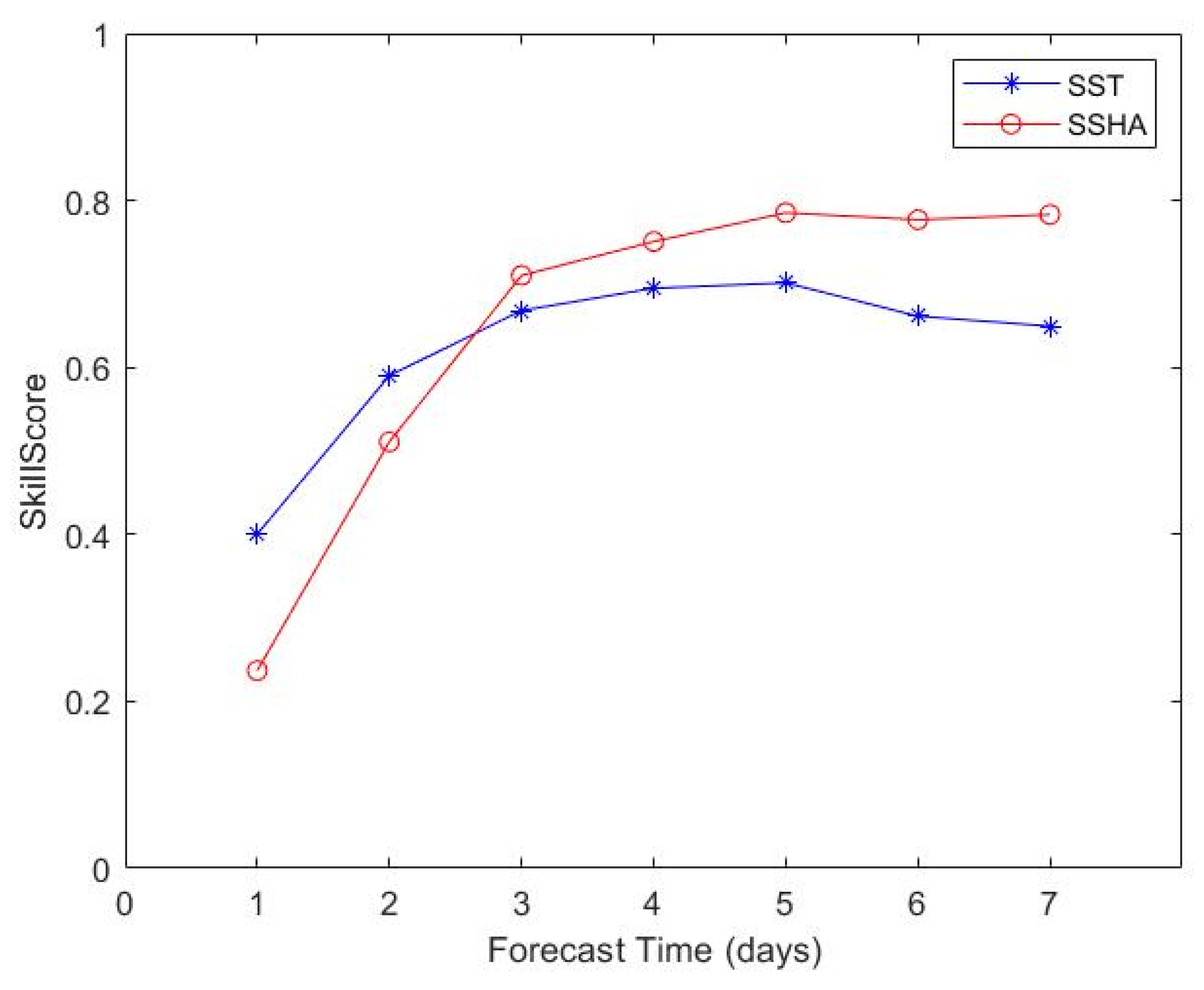
Figure 7 displays the results of the Skill Score (SS) experiments for both models. If SS is greater than 0, it indicates that the prediction result surpasses the PER. A value of 1 for SS signifies a perfect prediction. On the other hand, if SS is less than 0, it implies that the prediction result is inferior to the PER. By referring to Figure 7, it becomes evident that the MEOF-LSTM-D model exhibits SS values above 0 for both SSHA and SST during the entire prediction period. This outcome suggests that the MEOF-LSTM-D model outperforms the PER model in terms of prediction accuracy.

3.2.2. Case Study

Ultimately, the MEOF-LSTM-D prediction model predictive performance is demonstrated through the provision of examples. In the study area, Figure 8 displays a snapshot of MEOF-LSTM-D predictions and the corresponding truth fields for anomalous SSHA and anomalous SST. In the time series of the original dataset for testing, they represent 4 June, 6 June, 8 June, and 10 June 2019, respectively.

In Figure 8a,b, the observed and predicted results for SSHA and SST are presented. The MEOF-LSTM-D model integrates external and internal drivers. As evident from the figure, the MEOF-LSTM-D model has produced accurate predictions for the SSHA and SST in the Bohai Sea region, and there exists a significant correlation between the true values and the predicted values of the model. However, in regions of the study area with high (low) variable values, an unavoidable error exists between the prediction of the MEOF-LSTM-D model and the true value. For the construction of the prediction field, we choose the PC whose variance accounts for 89%, but this inevitably leads to the loss of some information. It is noteworthy that the MEOF-LSTM-D model exhibits a good level of prediction accuracy in regional evolution. In comparison to the current situation, the MEOF-LSTM-D model excellently portrays the evolving patterns of SSHA and SST.

4. Discussion

In this study, we consider the coordination between different variables in the real marine environment and the forcing from the atmosphere to the ocean. Using remote sensing data for the Bohai Sea region from January 1993 to December 2020, we focus on the interactions between oceanic variables and the feasibility of using atmospheric variables as predictors. In order to adequately assess the model performance, we utilize the initial 23 years of data for training the model, while the remaining 5 years of data serve as independent experimental samples for forecasting SSHA and SST for seven days.

The average water depth in the Bohai Sea is shallow, and the influence of external driving factors can not be ignored. To improve the prediction accuracy of oceanic variables, we considered introducing atmospheric variables into the model. Additionally, we designed three comparative experiments, one modeled without the influence of wind field and the other two modeled with the introduction of an external wind field, to simulate the strong and weak coupling of atmospheric and oceanic variables. Through these experiments, we identified a weak coupling approach that considers the interactions between oceanic variables and utilizes atmospheric variables as predictors.

Therefore, the MEOF-LSTM-D model utilizes MEOF analysis to examine the multivariate predictions for the sea surface, which includes SSHA and SST. The U and V components of SSW are employed as predictors to establish the prediction model for SSHA and SST. The MEOF-LSTM-D model achieves an RMSE of 0.011 m and 0.32 °C for SSHA and SST in the Bohai region, respectively, at the conclusion of the prediction period. The RMSE prediction for SSHA and SST is improved in the MEOF-LSTM-D model compared to the PER model and climatology results. Additionally, the model yields accuracy scores of approximately 0.95 for SSHA and 0.97 for SST, surpassing the performance of both the PER model and climatology results significantly. Throughout the prediction window, both the MEOF-LSTM-D model and PER model exhibit SS values that are above 0. The effectiveness of sea surface wind as a predictor for predicting SSHA and SST in the Bohai Sea was demonstrated by the MEOF-LSTM-D model consistently outperforming the PER model for SSHA and SST in the case study of the Bohai Sea.

In this study, our contribution lies in enhancing the accuracy of oceanic environmental variable prediction by incorporating the correlation between different variables within the real oceanic environment and accounting for atmospheric forcing on the ocean. This novel approach provides valuable insights and opens up new avenues for future research in the field of oceanic variable prediction.