A Virtual System and Method for Autonomous Navigation Performance Testing of Unmanned Surface Vehicles

Abstract

An overall framework of the virtual testing system has been established based on the analysis of the virtual testing requirements for autonomous navigation performance of unmanned surface vehicles (USVs). This system consists of several modules, including the environment module, motion module, sensor module, and 3D visualization module. Firstly, within the robot operating system (ROS) environment, a three-dimensional navigation environment was generated by combining actual wave spectra with Gerstner waves. By designing a power plugin for USV navigation, the system was made to reflects the coupled motion model of USVs in wind, waves and currents, along with predictive results. Regarding the four typical sensor information on USVs, the actual sensors were virtualized, and a simulation approach for virtual sensor information is provided. The three-dimensional visualization of USV’s motion enables the intuitive display and analysis of the virtual testing process. Based on the prediction of coupled motion characteristics in wind, waves and currents, the interaction between USVs and the virtual testing system has been realized. A platform for virtual testing experiments to determine the autonomous navigation performance of USVs was established, and the effectiveness of the platform was verified in terms of perception and environmental interference. In virtual environmental interference validation, the average amplitude deviation of the heave motion of USVs under sea state 3 reaches 0.74 m, and the average amplitude deviation of the pitch motion reaches 0.25 rad, showing the gradually increasing disturbance of the sea state. Finally, virtual testing experiments were conducted on a specific USV to evaluate its autonomous navigation perception performance, trajectory tracking performance, and autonomous obstacle avoidance. The evaluation results indicate that the platform can achieve the functionality of virtual testing for the autonomous navigation performance of USVs from the perspective of cost function, taking the reaction distance, regression distance, and obstacle avoidance time into consideration. A representative example is that the cost function deviation rates of overtaking obstacle avoidance between static and dynamic seas reach 5.11%, 8.98% and 18.43%, respectively. The gradually increasing data shows that the virtual simulating method matches the drifting-off-course tendency of boats in rough seas. This includes acquiring perception information of navigation and simulating the motion and navigation processes for visualization. The platform provides new means for testing and evaluating the autonomous navigation performance of USVs.

1. Introduction

USVs are extensively used in various fields, such as marine surveys and development, island replenishment and marine environmental monitoring. With the continuous expansion of USV applications in recent years, there is an increasing demand for the stability of autonomous navigation performance in complex marine environments. However, there are two main challenges in testing the autonomous navigation performance of USVs. Firstly, there is a significant risk in conducting tests in uncertain and complex environments before the overall application of USVs. Secondly, it is difficult to provide the required test environment with real-time wind, wave and current conditions in practical testing scenarios. If virtual simulation methods are employed to conduct some of the testing and training work on a simulation platform, they can effectively shorten the experimental cycle, reducing testing costs and risks [1].

Indeed, in the development of USVs, it is very common to utilize virtual simulation methods to conduct part of the testing and validation work. Phanthong et al. developed graphical simulation software to validate their proposed techniques for path replanning and underwater obstacle avoidance for USVs. This software is capable of simulating the control of USVs and generating virtual sonar images [2]. To validate the proposed obstacle-avoidance algorithm for USVs based on LiDAR, Villa et al. processed RGB maps and built a simulation testing environment by integrating the mathematical modeling of USVs [3]. To validate the proposed motion planning algorithm for USVs, Xinyong Wei [4] built a simulation environment in V-REP and established communication with Matlab through remote API functions, in this wayachieving the simulation testing of USVs. Dongdong Mu [5] utilized Matlab to conduct motion modeling and parameter identification for a single thruster-propelled USV. Subsequently, the proposed control strategies for heading control, path tracking, and trajectory tracking were validated through simulation. The aforementioned scholars specifically built simulation testing environments for USVs based on their own research areas. The testing projects conducted in these environments, however, tend to be relatively narrow and simple.

As autonomous navigation vehicles, USVs rely on the synergy of various functions such as path planning, image recognition, and motion control during their navigation process. If testing is conducted in isolated blocks, the overall system integrity may be overlooked. Additionally, unlike land-based unmanned systems, USVs are susceptible to environmental disturbances such as wind, waves and currents. Simulating the effects of wind, waves and currents is crucial for enhancing the realism of USV virtual simulation systems. Xiao G et al. adopted CFD tools to simulate the response of USVs regarding the wind–wave coupling effect, providing an assessment of ship-berthing-safety [6]. Gongxing Wu et al. established a mathematical operating system to simulate a ship berthing in a narrow port regarding different target parameters in three specific processes [7]. Maki. A et al. modeled the optimal berthing problem as a minimum-time problem, taking the collision risk into consideration, introducing the CMA-ES to solve the highly nonlinear problem robustly [8]. In the research aimed at enhancing the overall integrity and realism of virtual testing for USVs, Xinming Hu et al. designed a simulation system that incorporates wave disturbances. This comprehensive simulation system includes modules for the compass, simulated GPS, simulated LiDAR, and other components. Their proposed simulation solution is more comprehensive in nature [9]. Heins et al. developed a multiphysics simulation testing platform for the unmanned surface vehicle “Halcyon”. To achieve a more realistic ocean environment model, they combined multiple semiempirical wave spectra that can reflect the effects of ocean swells, local winds, surface currents and finite water depths [10].

In practice, in addition to enhancing the realism and effectiveness of virtual simulation, development efficiency and cost are equally important factors to consider in USV virtual simulation testing research. An effective approach to addressing these issues is to build upon existing platforms, which include commercial software and open-source simulation software. Unity3D, a representative of excellent commercial game engines, possesses powerful graphical processing capabilities and is widely used in ship visual simulation due to its ability to create realistic ocean scenes [11,12,13,14,15]. In addition to visual simulation, Wang et al. utilized the Unity3D engine to construct virtual ocean testing scenarios. They collected ocean image data in virtual scenarios to achieve image data enhancement under complex weather conditions and enable intelligent control training for USVs [16]. Zhou et al., combining Unity3D with Microsoft Visual Studio, built a hybrid simulation platform for testing USV path planning. They simulated the working effect of LiDAR within Unity3D, and the simulation platform corresponded well with actual USV experiments [17]. Indeed, OS and V-REP are widely used in robot simulation research. While they may not specifically provide a simulation environment for USVs, the variety of sensor simulations offered by these platforms greatly facilitates research in unmanned system simulation testing. Ødegaard developed a general USV motion control system based on the ROS framework to build an HIL testing platform for USVs. This system includes simulation modules for wind, waves and currents [18]. Building upon Ødegaard’s work, Børs-Lind created a maritime environment with both fixed and moving obstacles, providing a simulated interactive environment for USV models [19]. Bingham et al. developed the VRX simulator for the Maritime RobotX Challenge. This simulator, based on the ROS platform, enhances the simulation effects by incorporating various plugins into the original unmanned surface vehicle model [20]. Since then, several researchers have further enriched the functionality of USV simulation platforms built upon the aforementioned foundation [21,22,23].

A brief overview can be provided as follows: virtual simulation technology has greatly enabled the testing and development of USVs to be free from the restrictions of physical space, effectively improving the testing and development efficiency of unmanned vessels. Therefore, it is necessary to accelerate the research on virtual simulation testing technology for USVs. Additionally, compared to land-based unmanned systems, USVs are more significantly affected by environmental disturbances. Neglecting the impact of the environment will greatly reduce the effectiveness of testing. Therefore, reproducing the influence of external factors such as wind, waves, and currents as much as possible in a simulation platform is the key to researching the simulation testing technology of USVs. Furthermore, in order to improve the efficiency of simulation testing research, the universality and scalability of the simulation platform are also important indicators in the research of unmanned vessel simulation testing. Therefore, development based on existing platforms has become a trend in the research on virtual simulation for unmanned vessels.

Based on the analysis of the virtual testing requirements for the autonomous navigation performance of USV, the main goal of the research presented in this article was to establish an overall framework of the virtual testing system to evaluate the autonomous navigation perception performance, trajectory tracking performance, and autonomous obstacle avoidance for a specific USV. The novelties presented in this article includes the establishment of an overall framework of the virtual testing system, which includes the environment module, motion module, sensor module, and 3D visualization module, and a quantitative result can be produced by considering the monitoring data during the navigation process under different sea states and different maritime encounter scenes.

The remainder of this article is arranged as follows: in the second section, we presented the design of the virtual testing system for the autonomous navigation performance of USVs. In the third section, we implement virtual testing system within the ROS framework, in which environmental influences such as wind, waves and currents are incorporated to enhance the realism and effectiveness of the simulation. In the fourth section, we presented the autonomous navigation experiments that were conducted on a specific USV to evaluate its performance.

2. The Framework for a Virtual Testing System of the Autonomous Navigation Performance

2.1. Key Requirements Analysis for the Virtual Testing of Autonomous Navigation Performance

As an unmanned watercraft, autonomous navigation is a key aspect of the performance ofUSVs. To test the autonomous navigation capabilities of USVs, it is necessary to analyze and assess their performance in various areas, including but not limited to environmental perception, trajectory tracking and autonomous obstacle avoidance. These aspects are representative of the boat’s overall autonomous navigation ability.

Environmental perception is one of the core technologies of USVs, and it relies on sensor devices such as cameras, radar, and sonar to acquire three-dimensional data of the surrounding environment. The obtained data are then analyzed and processed to extract relevant information about the surrounding scene, including the type, position, velocity, and shape of targets. Therefore, constructing a testing environment for the environmental perception capability of USVs involves two main aspects: creating a simulated ocean environment and simulating sensor information. In a real ocean environment, there are wave surges and ocean currents, which differ from the detection environment on land. The local environment on the sea surface exhibits distinct non-planar characteristics. This non-planarity is also a major challenge in three-dimensional target detection at sea. A simulated ocean environment should be able to reflect such characteristics. In computer-generated ocean scenes, the features of targets can be output with perfect accuracy. However, in reality, no sensor is flawless. Sensor simulation should not only convert the information in the three-dimensional virtual scene into output signals of the sensors but also reflect the possible imperfections of the sensors themselves.

Trajectory tracking refers to the ability of USVs to navigate along a planned route. The difficulty of trajectory tracking varies significantly under different sea conditions. Unlike navigation in calm waters, environmental factors such as wind, waves and currents can cause USVs to drift and deviate from their intended trajectory. Ideally, the trajectory tracking capability should be able to handle random and complex disturbances. However, there are differences in the level of disturbances in different environments, making it inappropriate to compare them uniformly. Therefore, the virtual testing system should provide disturbances at different levels, specifically simulating various levels of sea waves, to conduct graded testing in different scenarios.

Autonomous obstacle avoidance refers to the ability of USVs to assess the status of encountered obstacles based on the sensor information they collect during navigation [24]. An avoidance decision system is then used to replay the trajectory and perform the necessary avoidance actions. This process involves both environmental perception and trajectory planning. Testing the obstacle-avoidance performance of USVs can involve designing various types of scenarios. Based on whether the obstacles are stationary or moving, it can be categorized as static obstacle avoidance or dynamic obstacle avoidance. Additionally, based on the number of obstacles, it can be classified as single-target obstacle avoidance or multitarget obstacle avoidance. The complexity of the navigation environment can also influence the maximum avoidance distance that USVs may encounter. As a result, the obstacle-avoidance performance of USVs may yield different outcomes in different scenarios. Therefore, the virtual testing system should provide the most effective testing scenarios to evaluate performance accurately.

Whether it is trajectory tracking testing or autonomous obstacle-avoidance testing, the motion simulation of USVs forms the foundation of the tests. As analyzed in Section 2, in addition to the driving force, gravity and buoyancy, USVs navigating on the water surface are also influenced by fluid dynamics, including fluid inertia and fluid viscosity. The effects of wind, waves and currents are ultimately manifested as forces acting on USVs. In the virtual testing system, the motion simulation of USVs is crucial for achieving realistic testing.

In summary, the key requirements for the virtual testing of USVs should include the following aspects: perception simulation, simulation of environmental disturbances, effective testing scenarios and the motion simulation of USVs.

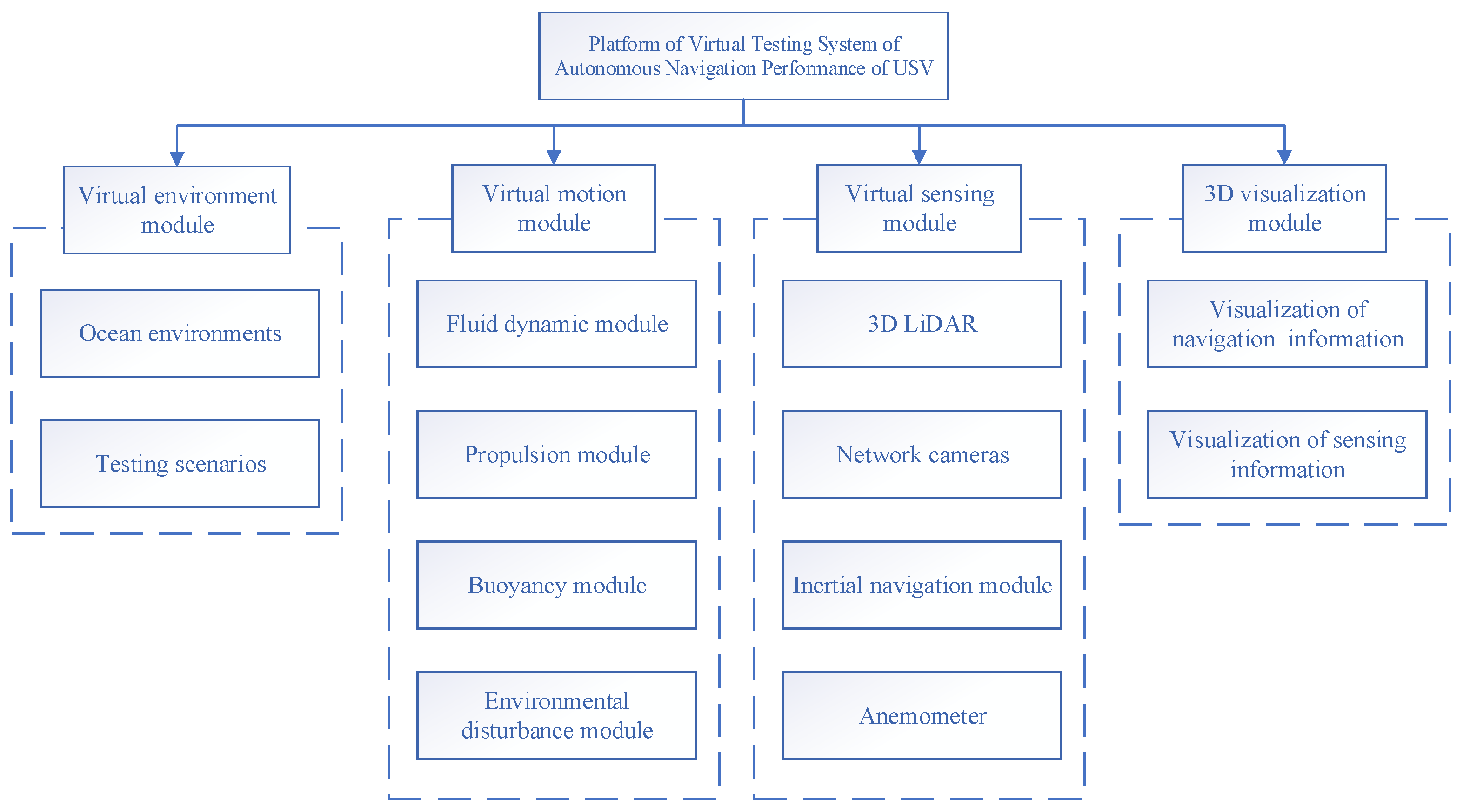
2.2. Design of the Framework for the Virtual Testing System

Based on the key requirements for the virtual testing of the autonomous navigation performance of USVs, the framework for the virtual testing system of the autonomous navigation performance of USVs is designed as shown in Figure 1.

According to Figure 1, the virtual testing system for the autonomous navigation performance of USVs can be divided into four modules: the virtual motion module, the virtual sensing module, the virtual environment module, and the 3D visualization module. The virtual motion module further consists of four submodules: the fluid dynamics module, the propulsion module, the buoyancy module, and the environmental disturbance module. The virtual sensing module includes the virtualization of four typical sensors: a 3D LiDAR, network cameras, an inertial navigation module, and an anemometer. The virtual environment module focuses on generating the sailing environment of USVs, including the generation of ocean environments and testing scenarios. The 3D visualization module is responsible for visualizing the navigation and sensing information during the virtual testing process.

3. Establishment of the Virtual Testing System

3.1. Design of the Framework for the Virtual Testing System

The whole system was established based on the ROS software framework. ROS, also known as the Robot Operating System, is designed on the foundation of the Linux system. It is widely used as a flexible framework to develop robot software. Gazebo is a three-dimensional physical simulating component of the ROS framework, consisting of a powerful physical engine and a graphical rendering engine. It can be conveniently programmed via a graphical interface and it is entirely open access software. We adopted a developing environment based on ROS Melodic with Ubuntu 18.04. The Gazebo component played a major role in the establishment of our virtual testing system.

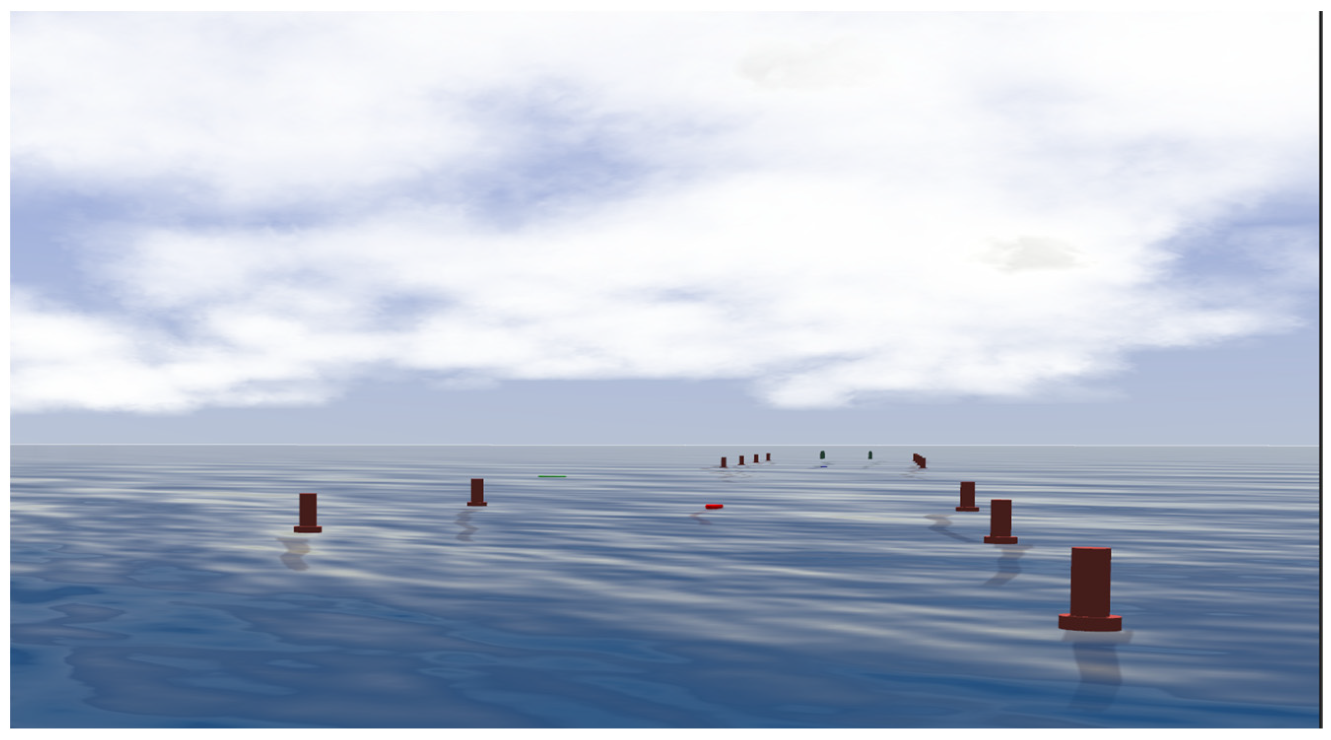
3.2. Generation of the Navigation World of USVs

The marine scene was not originally introduced by the Gazebo component; however, its modular structure allows it to be continuously enriched with plugins. Also a large number of researchers are constantly sharing models and code in the community. The RobotX project [25] then used Gazebo’s own rendering engine to generate a 3D ocean scene using the Gerstner wave model. The Gerstner wave model simulates water waves, in which each water molecule is moving in a circular motion, and the x and y values change simultaneously, allowing the effect of the entire water surface to gather in the peaks and spread out in the troughs of the waves. Assuming that the starting position of a point on the water surface in the horizontal direction is ${\overline{x}}_0=(x_0,y_0)$ and the starting position of the height is $h_0=0$, the position of the point according to the Gerstner wave principle is shown in Equation (1).

$$\{\begin{array}{l}\overline{x}({\overline{x}}_0,t)={\overline{x}}_0-{\displaystyle \sum _{i=1}^N{q}_i({\overline{k}}_i/k_i)A_i\sin (k_i\cdot {\overline{x}}_0-{\omega }_{i}t+{\varphi }_i)}\\ h({\overline{x}}_0,t)={\displaystyle \sum _{i=1}^N{A}_i\cos ({\overline{k}}_i\cdot {\overline{x}}_0-{\omega }_{i}t+{\varphi }_i)}\end{array}$$

(1)

where N is the number of the constituent waves, ${\overline{k}}_i$ represents the vectors of the angular wave number, $k_i$ is the horizontal direction of the angular wave number, and the angular wave number $k$ and the wavelength $\lambda$ follow the relationship $k=2\pi /\lambda$. The angular frequency and angular wave number can be related according to the linear infinite deep-water dispersion equation, which is ${\omega }^2=gk$. $A_i$ is the amplitude of the constituent waves. $q_i$ is the steepness coefficient in the rang of [0,1], where $q_i=0$ indicates that the waves are sinusoidal and $q_i=1$ indicates that the wave peaks present maximum steepness. ${\omega }_i$ represents the angular frequency. ${\varphi }_i$ is the random initial phase in the range of $0\sim 2\pi$.

Equation 1 describes the shape of the waves, which correlates with the characteristics of the constituent waves. In order to improve the realism of ocean simulations, we choose the dual-parameter P-M wave spectrum for sampling the characteristics of the constituent waves as Equation (2) shows below:

$$S_B(\omega )=\frac{1.25}{4}(\frac{{\omega }_p^4}{{\omega }^5}){(H_s)}^2\exp [-\frac{5}{4}{(\frac{{\omega }_p}{\omega })}^4]$$

(2)

where $H_s$ is the effective height of the wave and ${\omega }_p$ is the peak frequency. The navigation environment is generated, as shown in Figure 2.

3.3. The Virtual Motion Module of USVs

3.3.1. Fluid Dynamic Module

Gazebo does not provide users with the fluid dynamic simulation module, but it allows objects to withstand mechanical interaction. The fluid dynamic effect can be adopted as a plugin. In the MMG model, the hull of the boat, the propellers and rudders are regarded as independent components. The applied forces and moments on the unmanned vessel in each direction can be seen as the sum of their respective components, as shown in Equation (3).

$$\{\begin{array}{l}X=X_I+X_H+X_P+X_R\\ Y=Y_I+Y_H+Y_P+Y_R\\ N=N_I+N_H+N_P+N_R\end{array}$$

(3)

where the subscripts I, H, P, and R represent the fluid inertia force, fluid viscous force, propulsion force, and rudder force, respectively.

To establish the equation set, the fluid inertia force and viscous force of the USV should be evaluated. Here, we established a series of CFD experiments to realize the parameters in the formula set by conducting tests in oblique dragging and rotating arm conditions, which are widely used to specify the parameters of a ship [26]. Some of the experiment figures are shown in Figure 3.

In order to prove the accuracy of the CFD method, we carefully took the large container ship KCS (KRISO Container Ship) as the research object, based on the typical towing test to verify the CFD model for its scientific. Referring to the international standard data provided at the 2010 Gothenburg Symposium on Numerical Ship Hydrodynamics [27], a system of motion equations for unmanned boats, including fluid inertial force, viscous force and fluid power on the propeller was constructed, and the KCS coupled motion model was established by integrating the environmental disturbance factors of wind and wave currents. The results, which are listed in

Table 1. Experimental results of the CFD method’s accuracy.

	Number of Mesh Grids (Million)	Predicted Value of Drag Coefficient	Standard Value of Drag Coefficient Presented by the Gothenburg Symposium [27]	Deviation
Scheme 1	1.5464	0.003895	0.003711	4.96%
Scheme 2	3.6533	0.003821	0.003711	2.96%
Scheme 3	7.9518	0.003772	0.003711	1.64%

, show that the predicted drag coefficient deviation was within 4.96% through grid independence verification, which verified that the wind and wave current settings of the CFD model can be correctly used to examine the motion of the ship.

In the hydrodynamic simulation of USVs, two velocity arrays ${\overline{v}}_0$ and ${\overline{v}}_1$ are used to record the velocity of the USV in the previous and current time frame. The variable $t_0$ and $t_1$ are used to record the simulation time of the previous and current time frame. The hydrodynamic coefficients are used in the program as parameter variables for calculations. The acceleration $\overline{a}=({\overline{v}}_1-{\overline{v}}_0)/dt$ is repeatedly refreshed in the program loop. Then, hydrodynamic forces and moments are also refreshed with velocity and acceleration. At the very end of every time period, the ${\overline{v}}_0$ and $t_0$ are used to record the current time. The whole process is then repeated until the end of the simulation.

3.3.2. Buoyancy Module

If we only simulate the motion of the USV in the horizontal direction, ignoring that in the vertical direction, the interaction between the USV and the wave animation cannot be realized. On the other hand, a USV sailing on the surface of the water will be affected by the wave disturbance, leading to a rapid swaying on the surface of the water, which will have a great impact on the acquisition of the sensor data. This is also an environmental factor that plays a crucial role in the virtual testing of USVs.

An effective way to solve the above problem is to consider the effect of buoyancy on the USV, which is mainly related to the displacement at moderate-low speed, according to the Archimedes’ principle. Theoretically, all of the submerged surfaces of the hull in contact with water will be subject to water pressure. So, if the buoyancy force is applied to the center of gravity of the USV alone, the USV will lose its constraints in pitching and rolling. However, at the same time, the complex calculation method will significantly increase the time of buoyancy calculation, which will affect the real-time performance and synchronism of the simulation test. A fast and effective calculation method is to subdivide the draft volume of the USV into several constituent units, as shown in Figure 4a. The constituent units can be regarded as simple geometries, such as prisms, cones, etc., and the buoyancy calculation is carried out for each constituent unit separately. The buoyancy force on the constituent units $F_b$ will be applied to the calculation grid points, which are the midpoints of each constituent unit, as shown in Figure 4b.

The draft d on the constituent unit can be determined according to the distance from the water surface to the calculation grid point. We can set the maximum height of the constituent unit as $h$, the vertical drop from the calculation grid point to the bottom of the constituent unit as $h_1$, then the coordinates of the calculation grid point can be obtained via Gazebo at the current moment $(x,y,z_0)$. Simultaneously, the corresponding water surface coordinates $(x,y,z_1)$ can also be determined. Then, the draft of the current unit is as shown in Equation (4):

$$d=\{\begin{array}{ll}h& \left(z_1>h\right)\\ h_1-\left(z_0-z_1\right)& \left(z_0-h_1<z_1<h\right)\\ 0& \left(z_1<z_0-h_1\right)\end{array}$$

(4)

The vertical upward buoyancy force exerted on the constituent cells creates the effect of a moment at the center of gravity. Assuming that the longitudinal distance from the computational grid point to the center of gravity is $x$ and the vertical drop is $y$, the buoyancy force and moment exerted at the center of gravity of the USV are as follows:

$$\{\begin{array}{c}{Z}_b={\displaystyle {\displaystyle \sum }_{i=1}^n}{F}_{bi}\\ K_b={\displaystyle {\displaystyle \sum }_{i=1}^n}{F}_{bi}{y}_i\\ M_b={\displaystyle {\displaystyle \sum }_{i=1}^n}{F}_{bi}{x}_i\end{array}$$

(5)

where $n$ is the number of constituent units, $Z_{\mathrm{b}}$ is the total magnitude of the computational buoyancy force, $K_{\mathrm{b}}$ represents the rolling moment, and $M_{\mathrm{b}}$ represents the pitch moment. Theoretically speaking, with the increase in $n$, the calculation of buoyancy will be closer to the real situation, and the actual selection needs to take into account the calculation capacity of the equipment.

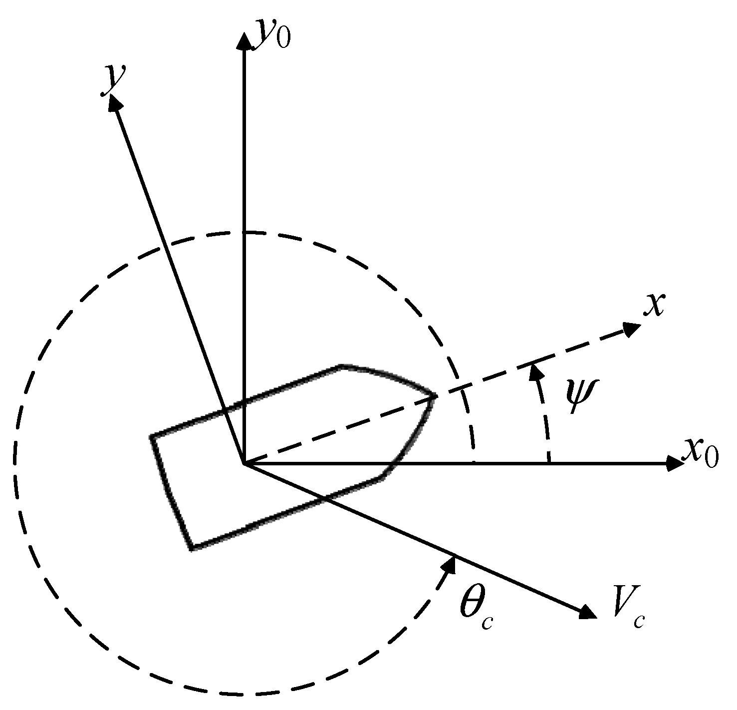
3.3.3. Environmental Disturbance Module

Environmental disturbances mainly refer to the effects of wind, waves and currents on the motion of a USV, where the environmental effects of wind and currents mainly cause the drifting motion of the USV, and we simulate them in the form of force. Waves mainly cause the swaying of a USV, which is modeled by applying buoyancy force as in Section 3.3.2.

The stochastic transformation process of the sea breeze is usually viewed as a superposition of a steady value and a time-varying value, i.e., for the wind speed at the time $t$, $V(z,t)$ can be decomposed into a mean wind speed $\overline{V}(z)$ and a perturbed wind speed $V_g(t)$ [28]. The mean wind speed is the average wind speed measured over a period of time., while the perturbed wind speed is a random value. The mean wind speed at a height of $z$ from the ground is calculated as shown in Equation (6) [29]:

$$\overline{V}\left(z\right)={\overline{V}}_{10}\frac{5}{2}\sqrt{\kappa }\ln \frac{z}{10e^{-\frac{2}{5\sqrt{\kappa }}}}$$

(6)

where, ${\overline{V}}_{10}$ is the average wind speed per hour at an altitude of 10 m above sea level and $\kappa$ is the sea surface drag coefficient, taken as 0.0026.

The Harris spectrum is widely used for variable wind speed acquisition, and the power spectral density is shown in Equation (7):

$$S\left(f\right)=\frac{4\kappa L{\overline{U}}_{10}}{{\left(2+{\tilde{f}}^2\right)}^{5/6}}$$

(7)

where $\overline{U_{10}}$ represents the average wind speed at a height of 10 m above sea level. In $\tilde{f}=Lf/{\overline{V}}_{10}$, $L$ is the scaling length of a value as 1800; while $f$ is the frequency in Hz.

According to the definition of spectral density, the time domain expression of the perturbed wind speed with N components is shown in Equation (8):

$$V_{\mathrm{g}}(t)={\displaystyle \sum _{i=1}^N\sqrt{2S(f_i)△f_i}}\cos (s{f}_{i}t+{\varphi }_i)$$

(8)

where $\mathrm{s}=2\pi$, $\Delta f$ is the frequency interval and ${\varphi }_i$ is the homogeneous phase.

Consideration of forces and moments generated by ocean currents can be achieved by converting the generalized velocities in Section 3.3.2 to relative velocities. The motion of ocean currents can be regarded as a horizontal flow with a relatively stable velocity. If the bow angle of a USV in the fixed coordinate system is set as $\psi$, the flowing velocity of current is set as $V_c$, and the flowing angle to be ${\theta }_c$, as shown in Figure 5, the components of the velocity of a USV, $u$ and $v$, are calculated as in Equation (9):

$$\{\begin{array}{l}u=u_r+V_c\cos ({\theta }_c-\psi )\\ v=v_r+V_c\sin ({\theta }_c-\psi )\end{array}$$

(9)

where $u_r$ and $v_r$ are the speed of a USV relative to the current.

3.4. Virtual Sensor Module

Sensors for USVs are designed to obtain their own motion status and the external environment. The virtual sensors module includes motion sensors and surrounding sensors. The motion sensors mainly include the virtual GPS and the inertial measurement unit, used to measure the location and the acceleration of the USV within its inertial coordinate system. Surrounding sensors are used to detect the surroundings around USVs, comprising a virtual LiDAR, a camera and an anemometer. In the virtual testing, the actual USV was placed in a static environment without moving. The virtual sensing information for the USV was provided in the virtual environment, triggering the USV to make corresponding control decisions based on its own algorithm according to the virtual sensing information. ROS provides a variety of sensor simulation plugins, which is convenient for USV’s perceptual simulation. At the same time, it was possible to simulate the acquisition error of the sensor by adding Gaussian noise to the output information of the sensor.

3.4.1. Motion Sensors Module

The virtual GPS collects the location of the virtual USV hull as a result of the USV-controlling algorithm, that is, the very position at the virtual moment where the virtual USV manages to arrive under the controlling methods and the environment disturbance effect. Meanwhile, the acceleration data of the hull during this voyage are sensed using the inertial measurement unit.

The GPS module was provided by the ROS Gazebo, which described the absolute position in the world framework of the virtual environment, and the relative position can be calculated with the knowledge of the origin of coordinates. The IMU data can also be inquired with the dynamic plugin of the Gazebo. This describes the real-time inertial data, the rotation data and the linear acceleration along three axes. An IMU usually encounters a random margin of error, including Gaussian noise and a random walk error. The error model of a single signal on the IMU is shown in Equation (10).

$$e(t)=b(t)+n(t)$$

(10)

where $n(t)$ is the Gaussian type error—a similar type of which will be mentioned in the next section—and $b(t)$ is the random walk error.

3.4.2. Surrounding Sensors Module

The virtual LiDAR and camera mounted on the virtual USV hull sense the virtual surroundings with a moving first-person perspective, obtaining information about the relatively moving obstacles. Meanwhile, the anemometer gains the wind direction and wind velocity, helping the USV to achieve a precise control. The virtual LiDAR we adopted in the testing system was modeled with simulated laser beams based on the principles of rotating lighting arrays. This also achieve a 360° horizontal field of view and a vertical field of 32°, containing 16 beams to achieve a 2° resolution as the actual lidar on the USV. The camera data in the perspective of the navigating USV can also be acquired with a preset resolution and refresh rate via subscribing to the topic published by the ROS system. The virtual anemometer was realized by subscribing to the message published by the ROS system, which was previously generated using the Harris spectrum that we adopted in the time domain expression in Equation (8).

As almost every LiDAR sensor may be possibly affected by noise during its operation, it is widely accepted that a Gaussian form of noise can be added to the three-dimension points cloud data to simulate the sensing noise, as described in Equation (11).

$$p(z)=\frac{1}{\sqrt{2\pi \sigma }}{e}^{\frac{-{(z-\mu )}^2}{2{\sigma }^2}}$$

(11)

where z represents the grey scale, $\mu$ represents the average value, and $\sigma$ represents the standard deviation in the statics domain.

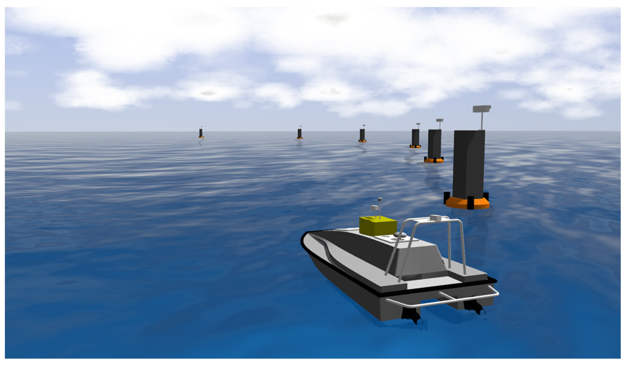
3.5. Three-Dimensional Visualization Module

The 3D visualization of USV navigation information seeks to fully demonstrate the process of the virtual testing of USVs, and to more intuitively establish the navigation status and control performance of USVs through multichannel view angles. The visualization of sailing attitude is shown in Figure 6, which can display the movement of the USV in the world in real time in Gazebo, and intuitively show the changes in the USV’s movement attitude under the manipulation and control instructions. The visualization of the virtual sensing information on the USV can be achieved with the help of the extensible QT programming, and the design of the visualization interface is shown in Figure 7.

3.6. Validation of the Effectiveness of the Virtual Testing System

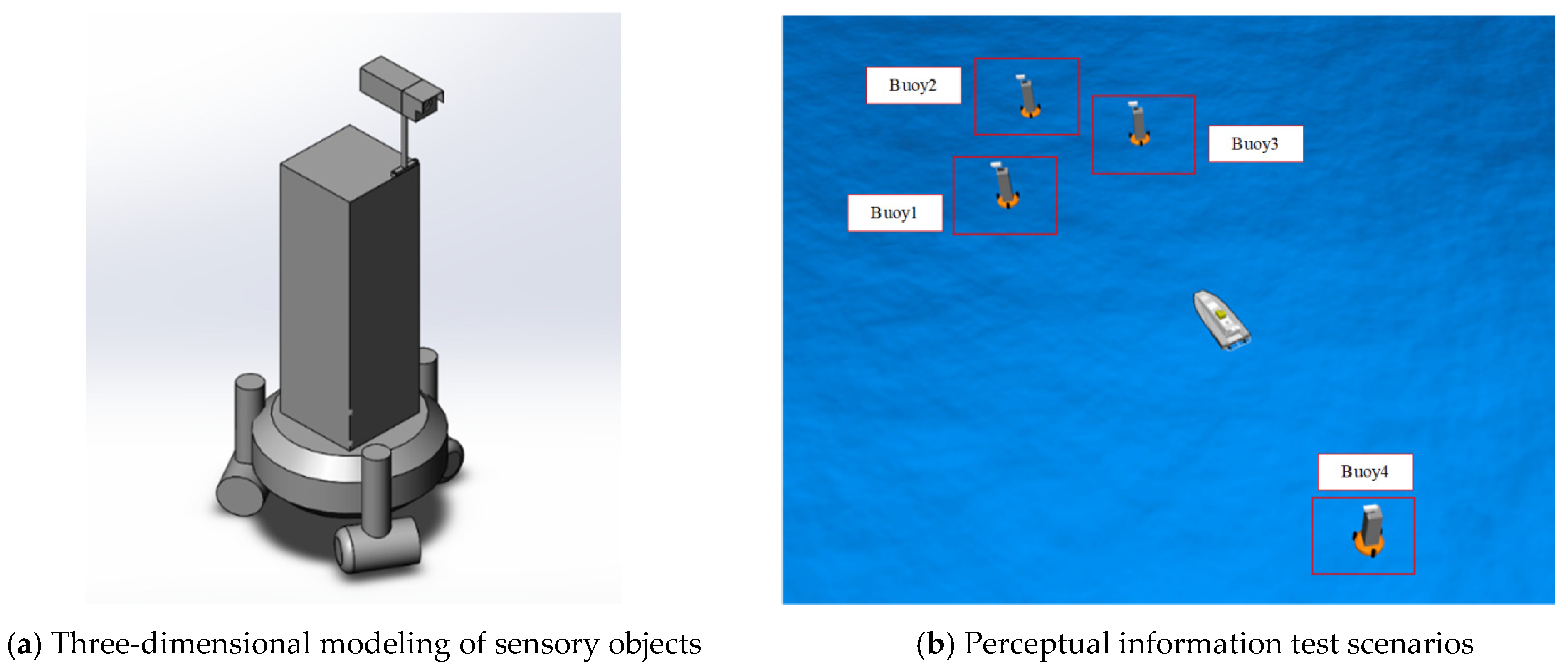
3.6.1. Validation of Perceptual Information Validity

The sensing information is the basis for the USVs to achieve environment perception, and three-dimensional environment perception mainly depends on the information collected by the three-dimensional LiDAR and camera. In order to ensure that the test virtual system can provide effective sensing information for the USVs, the virtualization effect of the LiDAR and the camera is analyzed. The sensing object and the sensing scene are shown in Figure 8, where the USV is stationary in the target sea area, and there are three buoy obstacles arranged in front of it, which are within the viewpoint capture range of the camera at the front of the USV. Additionally, there is one buoy obstacle arranged on its back side, which is within the viewpoint capture range of the camera at the rear of the USV. The obstacles in the scene are all within the scanning range of the 3D LiDAR.

By subscribing to the topics corresponding to the sensors, the USV can obtain the raw images and raw radar point clouds from the outputs of the camera and 3D LiDAR on the USV, as shown in Figure 9 and Figure 10.

The camera simulation is able to output the images of obstacles in the scene from the camera’s point of view, and the 3D point cloud reflects the relative position of the USV itself and the obstacles in the scene.

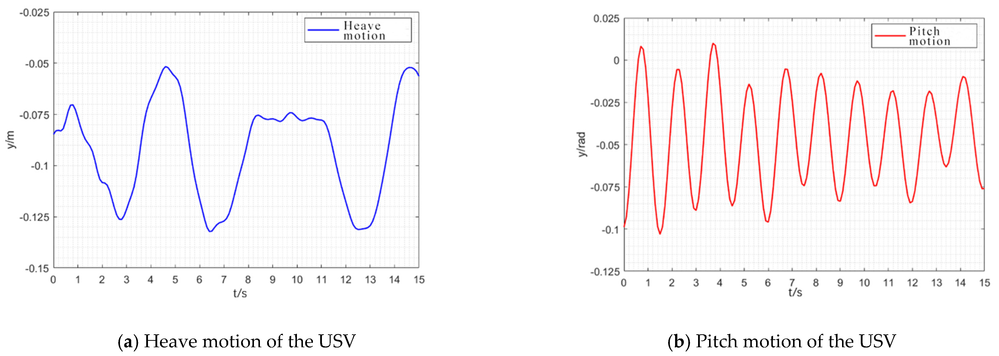
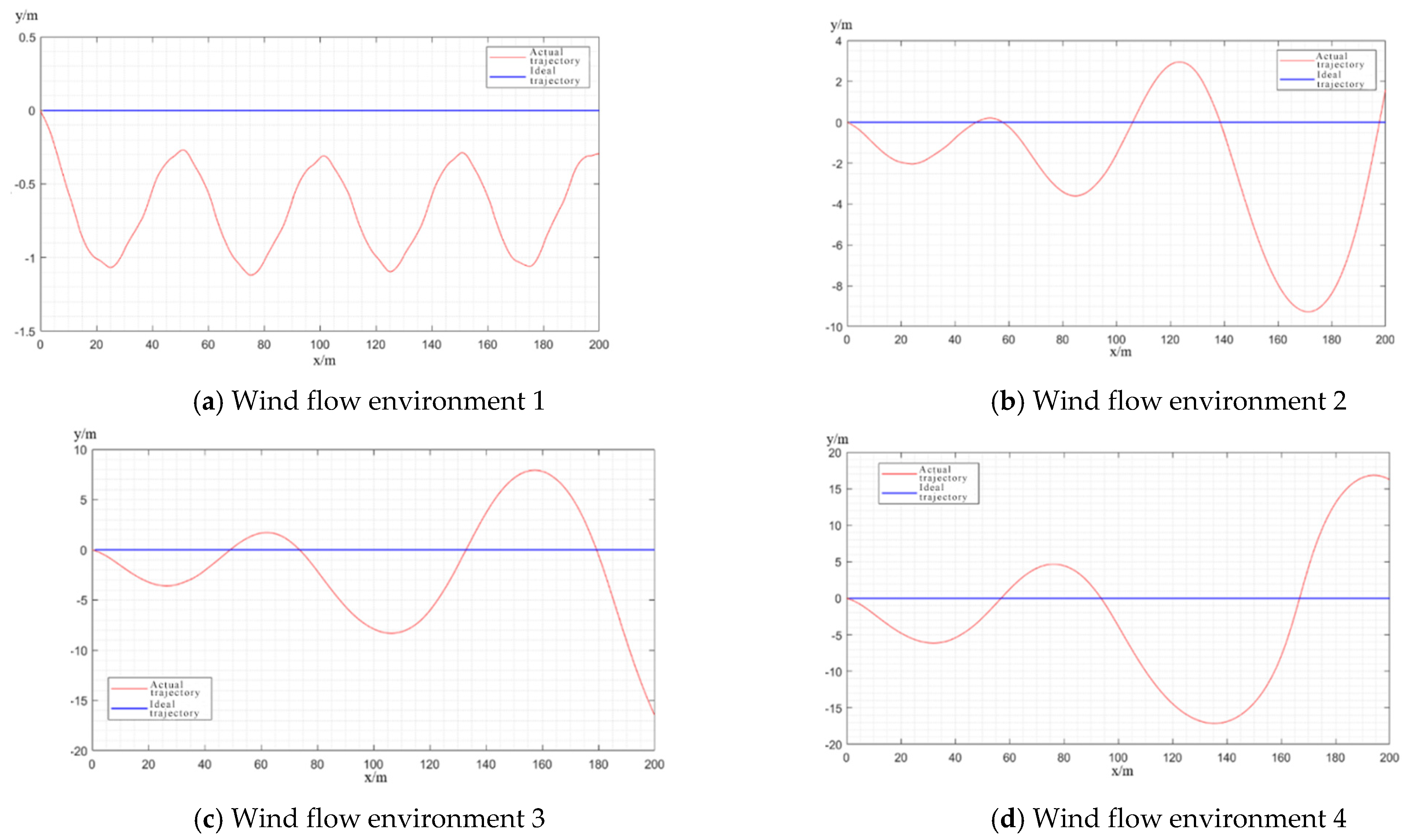
3.6.2. Validation of Environmental Interference Effectiveness

Virtual testing not only provides virtual sensing information to a USV, but also a test environment for the USV, including the effects of wind and moving currents, which is the core of virtual testing of USVs.

A three-dimensional marine environment is generated in the virtual testing system to simulate the heave and pitch motion of a USV on the waves by considering the effect of buoyancy on the USV. In order to realize the virtual testing of a USV under multiple sea conditions, the average height of the virtual waves is controlled to be 0 m, 0.1 m, 0.5 m and 1 m, corresponding to the actual sea conditions from 0 to 3, respectively. The USV is set to be free-floating with the changing influences without an initial speed, in order to exhibit the function of the environmental conditions. The sea surface is in a static water environment under the sea condition of 0, without the influence of wind and wave currents, and is not analyzed. Figure 11, Figure 12 and Figure 13 show how the attitude of a USV is affected by the waves under the sea states of 1, 2 and 3, respectively.

As shown in Figure 11, Figure 12 and Figure 13, the attitude of the USV is increasingly affected by the waves with the increase in the sea state level, and the average amplitude deviation of the heave motion reaches 0.07 m under a sea state of 1, 0.42 m under a sea state of 2, and 0.74 m under a sea state level 3.Meanwhile, the average amplitude deviation of the pitch motion reaches 0.08rad under the sea state of 1, 0.12rad under the sea state of 2, and 0.25 rad under a sea state 3. The virtual testing platform effectively simulates the reasonable influencing tendency on the attitude of a USV under different sea conditions.

Beyond testing with a static USV, the influence on a self-sailing USV are also inescapable. A typical USV straight line sailing situation was chosen for testing; in these cases, the USV needs to sail along a straight line to the destination under a set of parameters, and the total length of the voyage is 200 m. There are buoys arranged at the 100 m point and at the destination. The direction of the wind and water current is kept consistent and perpendicular to the preset trajectory. The environment conditions are designed with four speed groups; the speeds of the water current for conditions 1 to 4 are 0.1 m/s, 0.4 m/s, 0.7 m/s, and 1 m/s, respectively. The wind speeds are set as 4 m/s, 6 m/s, 8 m/s, and 10 m/s, respectively. The measurement and control terminals of the USV sends control commands to the virtual testing system to direct the USV in the virtual scene voyage to the destination under the influence of wind.

The ability of the USV to maintain a straight line can be judged according to the degree of deviation between the final trajectory and the preset one. Considering the maximum deviation distance and the average deviation distance of the USV in the straight line sailing, the root variance is used to evaluate the route keeping effect of the USV. Assuming that the USV’s coordinates under the current moment $i$ are $(x_i,y_i)$, and that the projection point of this location on the preset trajectory line is $(x_{ii},y_{ii})$, then the root variance $M$ can be presented by Equation (12):

$$M=\sqrt{\frac{{\sum }_i^n[{(x_i-x_{ii})}^2+{(y_i-y_{ii})}^2]}{n}}$$

(12)

The actual trajectories recorded for a USV in different environmental conditions of wind and current are shown in Figure 14.

As shown in Figure 14, the USV hull is affected perpendicularly by the wind flow, and the trajectory is largely trends in the direction of the wind. As the wind speed increases, the curvilinear nature of the sailing trajectory of a USV tends to be more significant, presenting the sinusoidal characteristics of longer cycles and larger amplitude. This also shows that the USV experiences an overshooting situation during its turning period, which can be described by accumulation the route offset driven by the disturbing wind and current. According to Equation (10), the root variance M of the USV in these four cases is 0.7331, 3.9158, 5.5025 and 10.1617, respectively, which shows that the platform regarding these disturbance models can gradually test out the difference in USV anti-interference ability under different parameter groups. The changing trends of deviations in the route-keeping performance of the USV agree with wave theory. While the virtual sailing performance also depends on the self-voyage algorithm of the USV, as it is expensive to test the algorithm in real sea conditions with a real vessel with specific parameter groups of sea state, a virtual system can reveal the pattern of USV performance in rough seas in this way. In summary, it can be seen that the virtual testing platform of USVs can effectively simulate the disturbance of the environment and achieve the virtual testing of USVs under different sea conditions.

4. Virtual Testing and Evaluation of the Autonomous Navigation Performance of USVs

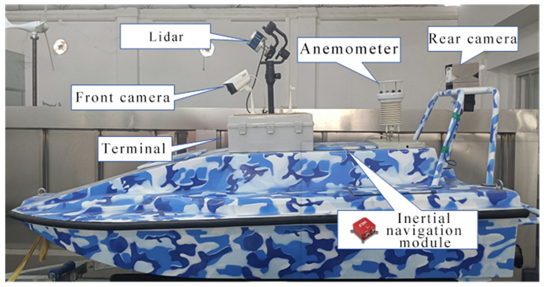
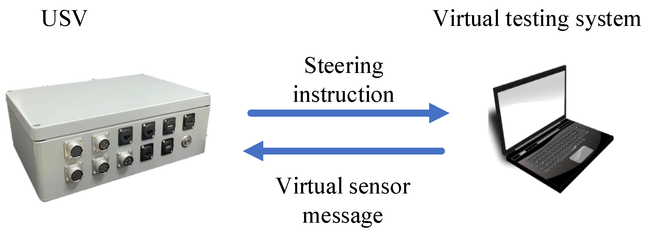
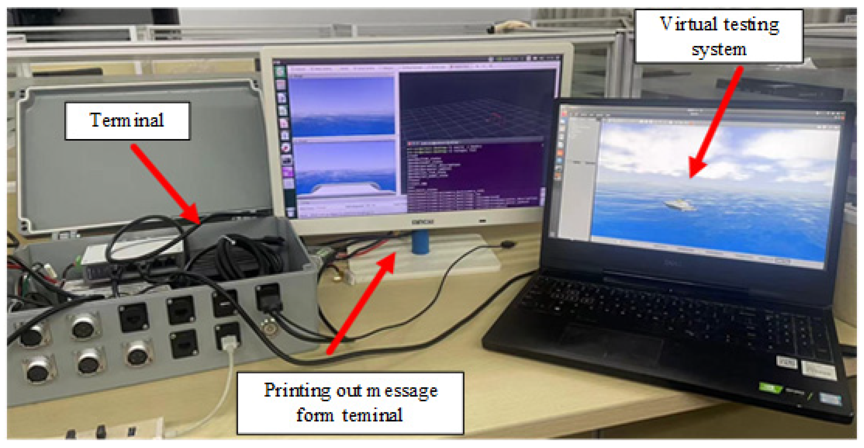
4.1. Virtual Testing Experimental Platform

Figure 15 shows the schematic structure of the tested USV. The sensors on the USV mainly include: a 3D LiDAR, an anemometer, a front camera, a rear camera, and an inertial navigation system. The 3D LiDAR adopts a Velodyne model 16-thread LiDAR with a horizontal field of view of −180~180° and a maximum and minimum field of view of 15° in the vertical direction. The camera is a 200 w pixel webcam from Hikvision, the inertial navigation system is a dual-antenna GNSS inertial navigation module, and the anemometer measures the wind direction and wind speed.

The measurement and control terminal is the control terminal of the USV, which adopts a Jeston Xavier processor, the CPU of the processor has an 8-core ARM architecture, the GPU adopts 512 CUDA Volta, and its computational performance is able to reach 30 TOPs under 30 W. The control algorithms, environment perception algorithms, and obstacle-avoidance algorithms on the USV are stored in the measurement and control terminal, which analyzes and processes the sensor information and provides the corresponding control commands.

The virtual interaction of the virtual testing platform specifically refers to the virtual interaction between the USV and the virtual testing system, as shown in Figure 16. In the test of the real boat, the USV acquires the external 3D environment information through its own sensors, while in the process of virtual testing, the USV under the test itself does not need to be within an actual marine environment. The virtual multi-sensor information is sent to the measurement and control terminal on the USV, which is equivalent to a USV in a specific sea state, and, according to the virtual environment information, it is entered into the real boat autonomous navigation intelligent perception algorithm. The control system of the real boat produces the maneuvering instructions, which are transmitted to the test virtual system in real time, guiding the USV to move in the virtual environment and releasing the new sensor information from the virtual sensor so as to realize the USV in the virtual testing and realize the testing effect of combining the real and virtual USV.

The prerequisite for real–virtual interaction is to establish the communication between the measurement-and-control terminal of the USV and the test virtual system. Since the measurement and control terminal of the USV and the test virtual system are within the environment of ROS, the sending and subscribing of the information topics can be realized through the topic mechanism. The laptop running the test virtual system is used as the host master, and the measurement and control terminal of the USV is connected to the master host through SSH. As shown in Figure 17, after the test virtual system runs on the host Master and opens the core service of ROS, the measurement and control terminal can judge its own sailing status in the virtual world by subscribing to the sensing information released in the test virtual system and returning the control instructions to the test virtual system.

4.2. Virtual Testing of Autonomous Navigation Performance of USVs

Autonomous obstacle-avoidance performance is the most representative type of performance in the autonomous navigation performance of USVs. The USV starts from a preset trajectory, identifies an obstacle and starts to avoid it, and then returns to the preset trajectory after successful avoidance, which is a process that tests the trajectory tracking performance of the USV as well as the perception performance of the USV. The navigational conditions encountered by the USV in the actual navigation process are complex and variable, and the virtual testing of a USV’s obstacle-avoidance performance needs to be able to provide effective obstacle-avoidance scenarios and corresponding test evaluation criteria [30]. In the literature, a quantitative evaluation method is proposed for the obstacle-avoidance performance of USVs [31]. According to the manuscript [32] by Hyo-Gon Kim, the obstacle avoidance of USVs can be divided into static obstacle avoidance and dynamic obstacle avoidance, among which dynamic obstacle avoidance includes three typical obstacle-avoidance scenarios, i.e., encountering, overtaking and crossing obstacle avoidance. Throughout these three scenarios, a line of sight (LOS) algorithm was used for USVs to avoid possible obstacle beyond the sea surface [33], and this algorithm was also selected to perform the obstacle-avoidance test.

The evaluation metrics for static and dynamic obstacle avoidance include the same indexes of reaction distance $d_{st}$ and obstacle avoidance time $T_{st}$. There are also other indexes: return distance $d_{st}{}^{\prime }$ in static scenes and avoidance minimum distance $d_{dy}^{\min }$ in dynamic obstacle scenes. The $d_{st}$ is the straight-line distance between the position of the USV and the obstacle at the moment when the USV starts the obstacle-avoidance maneuver. The $T_{st}$ is the time taken by USV from the start of the obstacle-avoidance maneuver to the end of the obstacle-avoidance process. $d_{st}{}^{\prime }$ and $d_{dy}^{\min }$ are, respectively, the straight-line distance and a minimum distance between the position of the USV and the obstacle, at the moment when the USV returns to the predetermined route after completing the obstacle-avoidance maneuver. During the above data-calculating process, every piece of distance data come from the original localization data of the USV monitored using the virtual GPS mounted on the USV model hull in the virtual testing environment.

According to the evaluation index corresponding to obstacle avoidance, we introduced a cost function which was proven to be effective and efficient in unmanned driving scenarios by [34] in order to comprehensively assess the obstacle-avoidance performance. The expression of the cost function $c$ for the obstacle-avoidance process is shown in Equation 13. Using the cost function method to evaluate the obstacle-avoidance performance the USV, we selected the USV with better obstacle-avoidance performance within a smaller cost function value, so as to quantify the obstacle-avoidance performance of the USV.

$$c=W_1{d}_1+W_2{d}_2+W_{3}T$$

(13)

where $W_1$, $W_2$ and $W_3$ are the weighting coefficients, $d_1$ is the response distance, $d_2$ corresponds to the regression distance and the minimum distance of dynamic obstacle avoidance, and $T$ means the time that consumed in the whole obstacle-avoidance period. Referring to the method of establishing weight coefficients in the literature [29,30], the ideal reaction distance is set to 20 m, and the safety distance of dynamic obstacle avoidance is set to 5 m, and the cost function of static obstacle avoidance $c_1$ and dynamic obstacle avoidance $c_2$ are calculated as shown in Equation (14).

$$\{\begin{array}{l}{c}_1=0.627(-d_{st}+20)+0.171d_{st}{}^{\prime }+0.202T_{st}\\ c_2=0.531(-d_{st}+20)+0.322(-d_{dy}^{\min }+5)+0.147T_{st}\end{array}$$

(14)

The test of static obstacle avoidance selects a single obstacle-avoidance scenario with visualization of a static obstacle-avoidance process. As shown in Figure 18, there exists a static obstacle buoy on the preset trajectory of the USV. The virtual sensors of the USV in real time send the current motion state of the virtual USV and the collected environmental information in real time to the measurement and control terminal of the USV. The USV enters into obstacle avoidance when the measurement and control terminal of the USV finds that there is an obstacle in front of it. When the USV returns to the preset route after avoiding the obstacle, obstacle avoidance process ends.

The static obstacle-avoidance performance of the USV was tested under sea states from 0 to 3 levels, and the test results of the evaluation indexes of USV’s static obstacle avoidance are shown in

Table 2. Test results of static obstacle-avoidance evaluation indexes of USV under each sea state.

Sea State	Reaction Distance (m)	Regression Distance (m)	Obstacle Avoidance Time (s)
0	19.12	18.13	21.31
1	18.76	20.32	22.05
2	19.02	20.91	22.93
3	18.87	24.18	24.32

according to the recording results of the background program.

According to the method of calculating the cost function for obstacle avoidance in Equation (12), the cost function for each sea state is obtained as 7.957, 8.706, 8.822, and 9.756, respectively.

Dynamic obstacle avoidance also includes the three cases of encounter, intersection, and overtaking. Figure 19 shows a visualization of the USV encounter obstacle-avoidance process, where an obstacle ship is approaching on the preset trajectory of the USV. The USV needs to avoid the obstacle ship and return to the preset route at the end of the avoidance process.

The USV was tested in the sea states from 0 to 3, and, according to the recorded results of the background program, the test results of the evaluation indexes of the USV in the encounter obstacle-avoidance process are shown in

Table 3. Evaluation index test results of the USV in the encounter obstacle-avoidance process.

Sea State	Reaction Distance (m)	Minimum Distance for Obstacle Avoidance (m)	Obstacle Avoidance Time (s)
0	19.09	6.46	12.43
1	19.39	5.89	13.05
2	19.01	5.67	12.89
3	19.79	4.98	15.21

.

Based on the calculation of the cost function for obstacle avoidance in Equation (12), the cost function for each sea state is obtained as 1.841, 1.955, 2.204, and 2.353, respectively.

Figure 20 shows a visualization of the USV undergoing intersection obstacle-avoidance process, where the sailing direction of the obstacle ship is perpendicular to the preset trajectory of the USV, and there is a probable crash on the preset trajectory. The USV needs to plan an obstacle-avoidance path to avoid meeting the obstacle ship and return to the preset trajectory after obstacle avoidance.

The USV was tested under sea conditions from 0 to 3, and according to the recorded results of the background program, the evaluation index test results of the USV for intersection obstacle avoidance are shown in

Table 4. Evaluation index test results of intersection obstacle avoidance for the USV.

Sea State	Reaction Distance (m)	Minimum Distance for Obstacle Avoidance (m)	Obstacle Avoidance Time (s)
0	19.29	5.61	15.65
1	19.47	5.32	16.12
2	19.05	5.57	16.73
3	19.26	4.54	18.21

.

Based on the calculation of the cost function for obstacle avoidance in Equation (12), the cost function for each sea state is obtained as 2.481, 2.548, 2.780, and 3.218, respectively.

Figure 21 shows a visualization of the USV overtaking the obstacle-avoidance test process. On the preset trajectory of the USV, there is an obstacle ship with the same heading, and the speed of the obstacle ship is lower than that of the USV, meaning that the USV needs to avoid and overtake the obstacle ship, and then return to the preset route after obstacle avoidance.

The USV was tested under sea states from 0 to 3, and, according to the recorded results of the background program, the evaluation index test results of USV overtaking obstacle avoidance are shown in

Table 5. Test results of evaluation indexes of the USV overtaking obstacle-avoidance process.

Sea State	Reaction Distance (m)	Minimum Distance for Obstacle Avoidance (m)	Obstacle Avoidance Time (s)
0	19.31	7.23	24.32
1	19.62	6.96	25.97
2	19.19	7.05	24.95
3	19.41	6.82	27.82

.

Based on the calculation of the cost function for obstacle avoidance in Equation (12), the cost function for each sea state is obtained as 3.223, 3.388, 3.511, and 3.817, respectively.

According to the experimental results of static obstacle avoidance and dynamic obstacle avoidance, it can be seen that the reaction distance of USV does not change too much in different sea conditions, and it is not much different from the ideal value, and the reaction distance is related to the perception performance of the USV, which proves that the USV obtains effective perception information. For the same obstacle-avoidance scenario in different sea conditions, obstacle-avoidance time changes are more significant; increasing with the increase in roughness of the sea state, indicating that the increase in the roughness of the sea state affects the control effect of USV. After static obstacle avoidance in rough seas, the USV struggles to return to its preset trajectory, and during dynamic obstacle avoidance, rough seas affect both the minimum distance of the obstacle avoidance and the return to the preset trajectory, indicating that the virtual testing platform effectively simulates the USV’s motion.

Based on the test results under static water conditions, when the cost function is not greater than 20% of the cost function under static water conditions, the autonomous navigation performance of the USV is considered to be rather resistant to environmental interference. The deviations of the cost function test results from those under a static sea state were calculated for sea states of 1 to 3, as shown in

Table 6. The test results: Deviation of cost function in a dynamic sea compared with a static sea.

Sea State	Static Obstacle Avoidance	Encounter Obstacle Avoidance	Intersection Obstacle Avoidance	Overtaking Obstacle Avoidance
1	9.41%	6.19%	6.7%	5.11%
2	10.87%	19.71%	12.05%	8.98%
3	22.6%	27.81%	29.7%	18.43%

.

The deviations under static obstacle avoidance are 9.41%, 10.87% and 22.6%, respectively; the deviations under encounter obstacle avoidance are 6.19%, 19.71% and 27.81%, respectively; the deviations under intersection obstacle avoidance are 6.7%, 12.05% and 29.7%, respectively; and the deviations under overtaking obstacle avoidance are 5.11%, 8.98% and 18.43%, respectively. This reveals that the deviation degree increased with the sea state getting more severe, which is normal and reasonable. Meanwhile, the deviations in the static obstacle-avoidance and the overtaking situation are barely smaller, which can be explained by the similarity of these two scenarios. The USV algorithm applies a direct acceleration in these two situations, helping the USV to suffer relatively less impact. In the other two scenarios, a deceleration order is applied first. A USV at a low speed is easily influenced by waves. Furthermore, an accelerating USV from a nearly idle status with wave disturbance requires more time and displacement to reach a target navigation status. So the relatively wider deviations in the encountering and intersection situation are also explainable. The calculated results overall reflects the difference in stability of the autonomous navigation performance of a USV under different sea states.

5. Conclusions

In this paper, for the needs of the virtual testing of the autonomous navigation performance of USVs, a virtual system for autonomous navigation performance testing of USVs is designed to complete the construction of the platform under the environment of ROS, add the environmental impact of wind and wave currents in order to improve the authenticity and validity of the simulation, and finally carry out the virtual testing of autonomous navigation performance of USVs with an actual USV as the object.

(1)

Under the ROS environment, a three-dimensional model of a USV is constructed, and a virtual system for testing the autonomous navigation performance of the USV is presented, which includes modules of environment, motion, sensors and visualization. The effectiveness of this virtual testing platform was validated in terms of the effectiveness of the sensory information and environmental interference. In the effectiveness test of sensory information, the virtual obstacles in the virtual testing environment can be perceived by the virtual sensors and relevant information can be obtained by the measurement and control terminal of the USV in the form of an RGB image and a 3D point cloud. In the effectiveness test of environmental interference, the average amplitude deviation of the heave motion of USV under the sea state 3 reaches 0.74 m, and the average amplitude deviation of the pitch motion reaches 0.25 rad, while the trajectory offset of the USV with the water current speed of 1 m/s and a wind speed of 10 m/s reaches 10.16 m. The average variance of the track deviation of the USV reaches 10.16 m. The mean square deviation of the USV under a current speed of 1 m/s and a wind speed of 10 m/s reaches 10.1617. The above results validate the effectiveness of the virtual testing platform in terms of perception ability and environmental interference.

(2)

A series of autonomous navigation experiments are carried out for the USV, testing obstacle-avoidance ability under static and dynamic situations with different sea states. The virtual testing experiments and evaluation results show that the virtual testing experimental platform is capable of evaluating the USV performance under different parameters of environmental conditions, revealing a tendency for navigation route deviation with the sea state become increasingly rough. The calculated results overall reflects the difference in stability of the autonomous navigation performance of USVs under different sea states.

References

1. Jin, J.; Zhou, Z.; Bo, Z.; Chen, Y.; Wei, X. Research on key technology of USV navigation simulation. J. Syst. Simul. 2021, 33, 2846–2853. [Google Scholar]
2. Phanthong, T.; Maki, T.; Ura, T.; Sakamaki, T.; Aiyarak, P. Application of A* algorithm for real-time path re-planning of an unmanned surface vehicle avoiding underwater obstacles. J. Mar. Sci. Appl. 2014, 13, 105–116. [Google Scholar] [CrossRef]
3. Villa, J.; Aaltonen, J.; Koskinen, K.T. Path-following with lidar-based obstacle avoidance of an unmanned surface vehicle in harbour conditions. IEEE/ASME Trans. Mechatron. 2020, 25, 1812–1820. [Google Scholar] [CrossRef]
4. Wei, X.Y. Research on Key Technology of Autonomous Local Obstacle Avoidance System for Surface Unmanned Craft; South China University of Technology: Guangzhou, China, 2019. [Google Scholar]
5. Mu, D. Research on Modelling and Motion Control Strategy of Unmanned Surface Vessel Propelled by Single Stern Machine; Dalian Maritime University: Dalian, China, 2020. [Google Scholar]
6. Xiao, G.; Tong, C.; Wang, Y. CFD Simulation of the Safety of Unmanned Ship Berthing under the Influence of Various Factors. Appl. Sci. 2021, 11, 7102–7114. [Google Scholar] [CrossRef]
7. Wu, G.; Zhao, M.; Cong, Y.; Hu, Z.; Li, G. Algorithm of Berthing and Maneuvering for Catamaran Unmanned Surface Vehicle Based on Ship Maneuverability. J. Mar. Sci. Eng. 2021, 9, 289–310. [Google Scholar] [CrossRef]
8. Maki, A.; Sakamoto, N.; Akimoto, Y.; Nishikawa, H.; Umeda, N. Application of optimal control theory based on the evolution strategy (CMA ES) to automatic berthing. J. Mar. Sci. Technol. 2020, 25, 221–233. [Google Scholar] [CrossRef]
9. Hu, X.; Zhang, X.; Zhong, Y.; Peng, Y.; Yang, Y.; Yao, J. Design and implementation of unmanned surface boat simulation system. J. Shanghai Univ. (Nat. Sci. Ed.) 2017, 23, 56–67. [Google Scholar]
10. Heins, P.H.; Jones, B.L.; Taunton, D.J. Design and validation of an unmanned surface vehicle simulation model. Appl. Math. Model. 2017, 48, 749–774. [Google Scholar] [CrossRef]
11. Craighead, J.; Murphy, R.; Burke, J.; Goldiez, B. A survey of commercial & open source unmanned vehicle simulators. In Proceedings of the 2007 IEEE International Conference on Robotics and Automation, Rome, Italy, 10–14 April 2007; pp. 852–857. [Google Scholar]
12. Wu, H.P. Real-Time Simulation of Ship Rocking Motion Based on Unity3D; Dalian Maritime University: Dalian, China, 2019. [Google Scholar]
13. Jiang, H. Research on the Development of USV View System Based on Unity3D; Wuhan University of Technology: Wuhan, China, 2016. [Google Scholar]
14. Lu, D.; Qiu, Y.; Xin, J. Simulation of ship manoeuvring motion based on Unity. Ship Eng. 2019, 41, 19–22. [Google Scholar]
15. Wang, Y. Research on Virtual Ship Simulation Based on Unity 3d; Zhejiang Ocean University: Zhoushan, China, 2019. [Google Scholar]
16. Wang, W.; Li, Y.; Luo, X.; Xie, S. Ocean image data augmentation in the USV virtual training scene. Big Earth Data 2020, 4, 451–463. [Google Scholar] [CrossRef]
17. Zhou, Z.; He, X.; Xu, L.; Qu, C. Simulation platform for usv path planning based on unity3d and a* algorithm. In Proceedings of the 2019 IEEE International Conference on Signal, Information and Data Processing (ICSIDP), Chongqing, China, 11–13 December 2019; pp. 1–6. [Google Scholar]
18. Ødegaard, E. Prototype of HIL Test Platform for Autonomous USV-Simulation of Vessel Dynamics; NTNU: Trondheim, Norway, 2017. [Google Scholar]
19. Børs-Lind, K.S. Prototype of HIL Test Platform for Autonomous USV-Simulation and Visualization of Vessel Surroundings; NTNU: Trondheim, Norway, 2017. [Google Scholar]
20. Bingham, B.; Agüero, C.; McCarrin, M.; Klamo, J.; Malia, J.; Allen, K.; Lum, T.; Rawson, M.; Waqar, R. Toward maritime robotic simulation in gazebo. In Proceedings of the IEEE OCEANS 2019 MTS/IEEE SEATTLE, Seattle, WA, USA, 27–31 October 2019; pp. 1–10. [Google Scholar]
21. Meng, J.; Humne, A.; Bucknall, R. A Fully-Autonomous Framework of Unmanned Surface Vehicles in Maritime Environments Using Gaussian Process Motion Planning. IEEE J. Ocean. Eng. 2022, 48, 59–79. [Google Scholar] [CrossRef]
22. Paravisi, M.H.; Santos, D.; Jorge, V.; Heck, G.; Gonçalves, L.M.; Amory, A. Unmanned surface vehicle simulator with realistic environmental disturbances. Sensors 2019, 19, 1068. [Google Scholar] [CrossRef] [PubMed]
23. Touzout, W.; Benmoussa, Y.; Benazzouz, D.; Moreac, E.; Diguet, J.P. Unmanned surface vehicle energy consumption modelling under various realistic disturbances integrated into simulation environment. Ocean Eng. 2021, 222, 108560. [Google Scholar] [CrossRef]
24. Yan, X.; Jiang, D.; Miao, R.; Li, Y. Formation control and obstacle avoidance algorithm of a multi-USV system based on virtual structure and artificial potential field. J. Mar. Sci. Eng. 2021, 9, 161–165. [Google Scholar] [CrossRef]
25. Smith, P.; Dunbabin, M. High-fidelity autonomous surface vehicle simulator for the maritime RobotX challenge. IEEE J. Ocean. Eng. 2018, 44, 310–319. [Google Scholar] [CrossRef]
26. Quan, Y.; Lau, L. Development of a trajectory constrained rotating arm rig for testing GNSS kinematic positioning. Measurement 2019, 140, 479–485. [Google Scholar] [CrossRef]
27. Larsson, L.; Stern, F.; Visonneau, M. Numerical Ship Hydrodynamics: An Assessment of the Gothenburg 2010 Workshop; Springer Science & Business Media: Berlin/Heidelberg, Germany, 2013. [Google Scholar]
28. Wenhua, L.; Jialu, D.; Yuqing, S.; Haiquan, C.; Yindong, Z.; Jian, S. Modeling and simulation of marine environmental disturbances for dynamic positioned ship. In Proceedings of the IEEE 31st Chinese Control Conference, Hefei, China, 25–27 July 2012; pp. 1938–1943. [Google Scholar]
29. Sørensen A, J. Propulsion and motion control of ships and ocean structures. Mar. Technol. Cent. Dep. Mar. Technology. Lect. Notes 2011. [Google Scholar]
30. Hong, X. A Quantitative Evaluation Method for Obstacle Avoidance Performance of Unmanned Ship. J. Mar. Sci. Eng. 2021, 9, 1127–1141. [Google Scholar]
31. Xiao, G.; Zheng, G.; Ren, B.; Wang, Y.; Hong, X.; Zhang, Z. A Test Method for Obstacle-Avoidance Performance of Unmanned Surface Vehicles Based on Mobile-Buoy–Shore Multisource-Sensing-Data Fusion. J. Mar. Sci. Eng. 2022, 10, 819. [Google Scholar] [CrossRef]
32. Kim, H.; Yun, S.; Choi, Y. Collision Avoidance Algorithm Based on COLREGs for Unmanned Surface Vehicle. J. Mar. Sci. Eng. 2021, 9, 863–872. [Google Scholar] [CrossRef]
33. Huang, Y. Research on Measurement and Control Technology for Automatic Berthing of Azimuth Thruster Unmanned Surface Vehicles; South China University of Technology: Guangzhou, China, 2021. [Google Scholar]
34. Wei, J.; Dolan, J.M.; Litkouhi, B. A prediction-and cost function-based algorithm for robust autonomous freeway driving. In Proceedings of the 2010 IEEE Intelligent Vehicles Symposium, La Jolla, CA, USA, 21–24 June 2010; pp. 512–517. [Google Scholar]
Figure 1. The Framework for the virtual testing System of the Autonomous Navigation Performance.
Jmse 11 02058 g001
Figure 2. The navigation environment.
Jmse 11 02058 g002
Figure 3. The CFD experiments to realize the fluid dynamic parameters for USVs.
Jmse 11 02058 g003
Figure 4. Principle of buoyancy calculation for USVs. (a) Division of buoyancy calculation area. (b) Buoyant forces acting on the calculation grid points.
Jmse 11 02058 g004
Figure 5. Bow angle ψ , Flowing velocity of current V c and flowing angle of a USV θ c .
Jmse 11 02058 g005
Figure 6. Visualization of the navigational attitude.
Jmse 11 02058 g006
Figure 7. Visualization of navigational information.
Jmse 11 02058 g007
Figure 8. Perceptual information test.
Jmse 11 02058 g008
Figure 9. Raw image information output from virtual camera.
Jmse 11 02058 g009
Figure 10. Raw point cloud of virtual LiDAR outputs.
Jmse 11 02058 g010
Figure 11. USV subjected to waves in a sea state of 1.
Jmse 11 02058 g011
Figure 12. USV subjected to waves in a sea state of 2.
Jmse 11 02058 g012
Figure 13. USV subjected to waves in a sea state of 3.
Jmse 11 02058 g013
Figure 14. Actual trajectories of the USV in different wind flow environments.
Jmse 11 02058 g014
Figure 15. USV experimental platform.
Jmse 11 02058 g015
Figure 16. Schematic diagram of the virtual testing process.
Jmse 11 02058 g016
Figure 17. Dual-computer communication configuration process.
Jmse 11 02058 g017
Figure 18. Visualization of the static obstacle-avoidance process for the USV.
Jmse 11 02058 g018
Figure 19. Visualization of the USV encounter-avoidance process.
Jmse 11 02058 g019
Figure 20. Visualization of the intersection obstacle-avoidance process for the USV.
Jmse 11 02058 g020
Figure 21. Visualization of the USV overtaking obstacle-avoidance process.
Jmse 11 02058 g021