Offshore Wind Energy Assessment with a Clustering Approach to Mixture Model Parameter Estimation

Abstract

In wind resource assessment research, mixture models are gaining importance due to the complex characteristics of wind data. The precision of parameter estimations for these models is paramount, as it directly affects the reliability of wind energy forecasts. Traditionally, the expectation–maximization (EM) algorithm has served as a primary tool for such estimations. However, challenges are often encountered with this method when handling complex probability distributions. Given these limitations, the objective of this study is to propose a new clustering algorithm, designed to transform mixture distribution models into simpler probability clusters. To validate its efficacy, a numerical experiment was conducted, and its outcomes were compared with those derived from the established EM algorithm. The results demonstrated a significant alignment between the new method and the traditional EM approach, indicating that comparable accuracy can be achieved without the need for solving complex nonlinear equations. Moreover, the new algorithm was utilized to examine the joint probabilistic structure of wind speed and air density in China’s coastal regions. Notably, the clustering algorithm demonstrated its robustness, with the root mean square error value being notably minimal and the coefficient of determination exceeding 0.9. The proposed approach is suggested as a compelling alternative for parameter estimation in mixture models, particularly when dealing with complex probability models.

1. Introduction

In the face of rapidly dwindling natural resources, the search for clean, renewable energy has gained urgency. The crucial requirement to pinpoint sustainable substitutes for fossil fuels and conceive of innovative strategies for energy development is more apparent than ever. Consequently, the research and application of renewable energy sources have become of prime interest. In current renewable energy alternatives, offshore wind energy is known for its reliability, consistency, and energy yield, making it a promising candidate [1,2]. As a measure against climate change, China’s 14th Five-Year Plan aims to achieve carbon neutrality prior to 2060. Key strategies within the plan involve the rapid advancement of non-fossil fuel energy resources, a substantial amplification in the deployment of wind and photovoltaic power technologies, and the systematic exploration and development of offshore wind energy capacities.

Estimating the wind energy potential of a specific site or area is crucial to determine the amount of electricity that can be produced. This aids in identifying the optimum wind turbine technology suitable for a given promising location. Therefore, the assessment of wind resources is vital in planning wind power projections. It establishes the framework for evaluating feasibility and estimating revenue, which are essential components for attracting the necessary investment. For conducting a thorough and accurate examination, it is typically recommended, where possible, to utilize a dataset spanning a decade or more [3]. For managing data of such extensive scale, a statistical distribution model is recommended. This model can elucidate the probability distribution of wind speeds and provide predictions for the generation of wind energy [4].

However, the presence of multiple concurrent weather systems indicates that accurately estimating wind resources might not be straightforward. Prior to initiating in-depth analysis, it is important to categorize wind data based on their originating wind-generating weather systems. This is due to the potential for winds produced by different weather systems to display unique probabilistic characteristics [5]. This notion is especially prevalent when it comes to the estimation of extreme wind velocities. Gomes and Vickery [6] introduced a technique to compute probability estimates for extreme wind velocities in mixed climatic conditions. This method requires an exhaustive investigation of each significant meteorological incident responsible for wind generation. The evaluation of wind speeds follows a three-step process. First, various wind phenomena, including extra-tropical depressions, thunderstorms, and gust fronts, are distinctly identified. Subsequently, the respective distribution of wind speed for each event is determined. The final phase combines these distributions into a unified mixed distribution representing the wind speed. Cook et al. [7] further improved this method by incorporating recent advancements in extreme value analysis.

The practice of categorizing based on weather patterns is also employed in simulating wave fields within mixed climate scenarios [8,9]. The process initiates with the collecting and preprocessing of historical predictor and predictand data. Next, weather types associated with synoptic circulation conditions are classified and identified. A probability distribution model is then fine-tuned to align with the predictand pertinent to each weather type. The final step involves the computation of return periods, factoring in the occurrence likelihoods affiliated with each distinct weather category. Assuming the homogeneity of extreme wave height data originating from a distinct meteorological pattern, Solari and Alonso [10] employed clustering algorithms to categorize weather formations. This enabled the identification of homogenous populations allied with each pattern. Consequently, the traditional extreme value distribution could be applied to each homogenous subset. The overall distribution was then configured using the multivariate Poisson model. This technique was then applied by De Leo et al. [11] to examine severe sea storms across Italy’s coastal areas.

The essential task in executing this methodology lies in categorizing wind data in the context of weather systems. To facilitate this, a range of classification algorithms have been put forward. Lombardo et al. [12] proposed an approach for the automated classification of winds, distinguishing between thunderstorm and non-thunderstorm origins. This method utilizes meteorological data, along with the initiation and cessation timings of thunderstorms. De Gaetano et al. [13] proposed a semi-automated technique for the discernment and categorization of extreme wind phenomena using a blend of systematic quantitative measures alongside specific qualitative decisions.

It is worth noting that a unified standard for the classifying meteorological patterns is still lacking. The utilization of diverse classification standards often leads to significantly divergent outcomes. The effectiveness of classifying wind events into disparate groups to facilitate comprehensive analysis can be challenged if the preliminary segregation process lacks equivalent precision [14,15]. For instance, despite the customary division of wind events in the scholarly literature into extra-tropical depressions and thunderstorms, Kasperski [16] underscored the existence of an intermediate third class of occurrences. Adding to this perspective, Choi and Tanurdjaja [17] suggested that categorizing the mixed weather systems based on their scale, namely into large-scale and small-scale categories, would be a more suitable approach. In addition, measuring wind speeds from typhoons is very difficult due to their relatively scarcity compared to other events. A given site may confront a mere one or two typhoons in a season, which inevitably leads to insufficient data required for a precise quantification of extreme wind speeds [6].

An alternative approach for data clustering involves using the mixture distribution model. This approach affords adaptability in managing clusters with diverse sizes and internal correlation architectures, rendering it a potentially superior choice over methods like k-means clustering for certain applications [18,19,20]. The premise of the mixture distribution methodology is that the larger population is divided into multiple subgroups, each following its own unique probability distribution. Following this, data clustering is accomplished by associating each data point with the component exhibiting the highest computed posterior likelihood of membership for that specific data point. This turns clustering into an endeavor to estimate parameters within the mixture model [21,22]. Mixture distribution models have gained widespread acceptance in the analysis of wind and wave data due to their flexibility [23,24,25,26,27]. Research has indicated that these models, comprising a blend of individual probability distributions, offer a robust approach to analyzing data with complex structures, that surpass the capabilities of a single distribution. Their adaptability proves advantageous in addressing the patterns in wind and wave data, making them well-suited for predictive analysis. This remarkable versatility is of utmost significance in applications such as wind power generation, where precise wind speed forecasts are indispensable for optimizing energy production efficiency [28,29]. Consequently, mixture distribution models have emerged as a potent method in the pursuit of accurate and efficient utilization of renewable energy sources.

Although mixture distribution models offer a degree of flexibility and adaptability, they are accompanied by computational complexities that introduce significant challenges, especially in parameter estimation. Conceptually, the direct maximization of a mixture model’s likelihood function to estimate its parameters might appear viable. However, the complexity of doing so often becomes a limiting factor due to the computational challenges in these models. In addressing mixture distribution problems, the expectation–maximization (EM) algorithm is often chosen. This preference can be primarily ascribed to its advantageous characteristics, such as numerical robustness, guaranteed global convergence, and straightforward implementation [30]. In many simple scenarios, the EM algorithm is commonly relied upon for its capacity to yield practical solutions. Nevertheless, it might not always identify the global optimum in a mixture distribution context. Additionally, the computational demands of such a process can be very complex and the pace of convergence could prove to be unsatisfactorily slow [31].

Usually, wind energy resources can be assessed using variables such as wind power density (WPD). This often involves parameters like wind speed and air density. Please note that although air density is often assumed to remain constant in many previous studies, the value of this variable could be affected by many factors, such as altitude, temperature, pressure, and humidity. Research indicates that it is not reasonable to assume air density as constant when forecasting wind energy resources [29]. Therefore, this study aims to evaluate wind energy resources by establishing a bivariate probability distribution for wind speed and air density. However, the co-existence of different meteorological systems presents considerable challenges for wind energy assessment. Current methods, proposed by Gomes and Vickery [6], require a thorough examination of individual meteorological events, and the lack of standardized classification meteorological patterns often yields inconsistent results. Additionally, although mixture distribution models provide adaptability and flexibility for mixed data clustering, significant computational challenges can be introduced in parameter estimation. Even established approaches, such as the EM algorithm, often encounter difficulties when handling complex probability distributions. In light of these challenges, this research aims to apply the principles of cluster analysis with the primary goal of partitioning a mixed dataset into distinct groups or classes. Each of these groups or classes is characterized by a homogeneous pattern of probabilistic statistical properties. By transforming the challenge of mixture distribution models into dealing with multiple single-mode probability distributions, the problem of solving the complex likelihood function can be averted. This approach enables a more precise wind resource assessment using the mixture distribution model. The rest of the paper is structured as follows. Section 2 details the unsupervised classification approach and the implementation of the EM algorithm for mixture distribution. In Section 3, experiments are presented to validate the efficacy of the proposed algorithm in clustering data with diverse statistical characteristics into uniformly distributed groups. Moving on to Section 4, the proposed classification approach is applied to model the mixture bivariate distribution of wind speed and air density, subsequently enabling the assessment of wind power potential based on the constructed joint distribution. Section 5 delves into a comprehensive discussion of the clustering algorithm. Finally, Section 6 offers concluding remarks summarizing the study’s major findings.

2. Methodology

2.1. Expectation–Maximization Algorithm

Considering a group of d random variables labeled as U = (X₁, X₂, …, X_d) with n observations, the mixture probability density function, composed of J components for these random variables (X₁, X₂, …, X_d), can be expressed as follows:

$$f\left(U\left|\xi \right.\right)={\displaystyle \sum _{j=1}^J{\omega }_j{f}_j\left(U\left|{\theta }_j\right.\right)},$$

(1)

where ω_j signifies the weight assigned to the j-th component, and θ_j denotes the parameters that describe the distribution model for that component. The set ξ includes all the unknown parameters in the distribution model.

Normally, when trying to find the maximum likelihood estimate, the goal is to identify parameters that optimize the likelihood function. This can be accomplished by deriving the logarithmic form of the likelihood function L(ξ), given by

$$\frac{\partial L\left(\xi \right)}{\partial \xi }=0.$$

(2)

Nonetheless, the relationship between the likelihood function and the parameters in a mixture model can be significantly complex, further complicating the computations. As the number of components increases, so does the flexibility of the mixture model, yet this simultaneously amplifies difficulties in parameter estimation. The EM algorithm provides an iterative method designed to identify proximate solutions by maximizing the expected value of the log-likelihood function of the given probability density function:

$$\widehat{\xi }=\arg \max \mathrm{E}\left(L\left(\xi \right)\right).$$

(3)

The application of the EM algorithm can be divided into two well-defined stages: the expectation (E) step and the maximization (M) step. In the r-th iteration, the task of the E-step is to calculate the conditional expectation of the log-likelihood function, termed the Q function:

$$Q\left(\xi \left|{\xi }^{\left(r-1\right)}\right.\right)={\mathrm{E}}_{{\xi }^{\left(r-1\right)}}\left[L\left(\xi \right)\right].$$

(4)

Following this, the M-step in the r-th iteration tries to find the maximal value of Q(ξ|ξ^(r−1)) and update the approximation of ξ^(r−1) to ξ^(r). The EM algorithm seeks ξ by consistently executing E- and M-steps until the divergence in consecutive log-likelihood values narrows to an acceptably minute degree:

$$\left|L\left({\xi }^{\left(r\right)}\right)-L\left({\xi }^{\left(r-1\right)}\right)\right|<\epsilon \hspace{1em}\left(\epsilon >0\right).$$

(5)

One appealing feature of this maximum likelihood estimator, as substantiated by Dempster et al. [32], is its non-decreasing log-likelihood function in each EM algorithm iteration. This implies that the EM technique gradually refines estimates with each step. Instead of tackling the direct optimization of L(ξ), the EM algorithm continuously aims to maximize Q(ξ). Nevertheless, this task of maximization can still be challenging, particularly when dealing with a substantial quantity of random variables, which could lead to a highly intricate joint probability density function and, in turn, a complex Q function [31].

2.2. Clustering Algorithm

Clustering refers to the organization of a range of objects into categories in such a way that those within the same category exhibit a higher degree of mutual similarity compared to those within alternate categories. In this respect, cluster analysis does not necessitate pre-established groups for data allocation, thereby operating as an unsupervised learning technique. In the framework of this unsupervised approach, information is extracted from the data independently of any pre-established labels or categories. A range of algorithms, including the k-means algorithm [33,34], density-based spatial clustering of applications with noise (DBSCAN) [35,36], and balanced iterative reducing and clustering using hierarchies (BIRCH) [37,38], can be utilized to achieve this. Each brings a unique perspective to the definition of a cluster and methods for their efficient detection. Common depictions of clusters incorporate groups characterized by minimal distances between members or densely populated areas within the data space.

This research employs the maximum likelihood function as the measure of distance to develop a novel clustering algorithm. The algorithm operates by dynamically modifying the classification of each data point to maximize the total maximum likelihood value for the mixture distribution model. The foundation of this method is that, through continuous refinements and optimizations, an optimal group structure can be accomplished wherein each data point is correctly categorized. A summarization of the steps undertaken in the execution of this innovative clustering algorithm is presented as follows:

Step 1: Define the probability density functions and number of clusters. Prior to initiating the clustering procedure, the probability density function for each respective cluster should be specified. Subsequently, the number of clusters J, is determined for the execution of the algorithm. This will result in the partitioning of the mixed data into J distinct clusters, with J being an arbitrary value, and the precision of clustering will vary accordingly. The identification of mixture components is a critical step, and three widely recognized techniques are employed for this purpose [39]. The first approach involves the assessment of the distribution’s modes [40], a process demanding the clear separation of mixture members. The second technique relies on the method of moments [41], while the third method centers on likelihood, which has become a primary mechanism for determining mixture components [42,43]. Using information criteria for the assessment of clusters through likelihood offers a straightforward and efficacious method [44]. In this application, the Bayesian information criterion (BIC) is selected to ascertain the optimal value of J, as guided by the findings of Dziak et al. [45]:

$$BIC=-2L\left(\xi \right)+n_{\xi }\log n,$$

(6)

where n_ξ denotes the number of unknown parameters in the mixture model, and n represents the size of the observed data. The optimization of the cluster number is thus achieved through the minimization of Equation (6).

Step 2: Initiate the clustering algorithm. For this purpose, random starting values are employed to specify the preliminary estimates for ξ, commencing by partitioning the data into J arbitrary groups, respective of the J distinct clusters within the mixture model. Within this construct, any subsample affiliated with cluster j is inferred to originate exclusively from the j-th sub-model of the mixture distribution. Utilizing this strategy, the observations contained within cluster j enable the derivation of the initial parameters specific to the j-th sub-model. This approach further allows the initial value ω⁽⁰⁾ to be aligned with the weight attributed to each cluster:

$${\omega }_j^{\left(0\right)}=\frac{n_j}{n},$$

(7)

where n_j represents the number of data points allocated to cluster j.

Step 3: Evaluate the log-likelihood assignment. For each observation, the log-likelihood L(ξ) is computed with regard to its allocation to each cluster. Should the assignment of the observation to a specific cluster increase the log-likelihood value, it is then classified into that cluster. Concurrently, the weights of the clusters and parameters tied to the corresponding sub-models are updated.

Step 4: Assess convergence. Calculation of the log-likelihood L^r(ξ) corresponding to the current cluster classification is performed, and contrasted with L^r−1(ξ), the value from the preceding iteration. If the alteration in value is less than a specific threshold,

$$\left|L^r\left(\xi \right)-L^{r-1}\left(\xi \right)\right|<\epsilon \hspace{1em}\left(\epsilon >0\right),$$

(8)

or if a predetermined number of iterations have been executed, the algorithm is terminated.

Step 5: Steps 3 and 4 are reiterated. The procedure alternates between the cluster assignment and update phase (Step 3), with a continual assessment for convergence at each iteration (Step 4).

Step 6: The final cluster assignment for all data points is returned, along with the parameters constituting the mixture model.

To provide a clear and concise understanding of the steps involved in our proposed clustering algorithm, a flow chart detailing the procedure is introduced in Figure 1. Drawing from the principles of unsupervised learning, the approach presented in this study integrates probabilistic statistical techniques for the purpose of segmentation of mixed datasets. The algorithm dynamically adjusts the classification of individual data point categorization to maximize the overall maximum likelihood value of the mixture distribution model. Through a process marked by iterative refinement and optimization, the algorithm facilitates accurate categorization, thereby establishing an optimal structure of groupings. The method’s application provides an innovative and pragmatic framework for the estimation of the parameters characterizing the mixture distribution model.

2.3. Wind Energy Assessment

Considering the significance of considering the effect of air density in wind energy production, the joint distribution of wind speed and air density is adopted to perform the wind resource assessment in the present application. The wind power density, a critical metric for energy evaluations, signifies the abundance of available wind resources at a particular location. This metric is formulated as given by the equation:

$$WPD=\frac{1}{2}{\displaystyle {\int }_{v_{\mathrm{c}\mathrm{u}\mathrm{t}-\mathrm{i}\mathrm{n}}}^{v_{\mathrm{c}\mathrm{u}\mathrm{t}-\mathrm{o}\mathrm{u}\mathrm{t}}}{\displaystyle {\int }_{{\rho }_{\min }}^{{\rho }_{\max }}\rho v^{3}f\left(v,\rho \right)}d\rho }dv.$$

(9)

In this equation, ρ is the air density at the predetermined hub height, while v represents the wind speed at the same elevation. ρ_min and ρ_max signify the lower and upper bounds of air density, respectively. Moreover, v_cut−in and v_cut−out are parameters indicating the operational thresholds of the wind turbine for initiating and ceasing power generation, respectively. These two parameters define the range of wind speeds at which efficient conversion of wind energy into electrical energy is actualized by the turbine.

The annual energy production (AEP) serves as a metric to quantify the energy output of a wind turbine and holds crucial importance for the economic feasibility assessment of wind energy projects. Through the application of the prescribed bivariate joint distribution model, the AEP is formulated as follows:

$$AEP=n_T{\displaystyle {\int }_{v_{\mathrm{c}\mathrm{u}\mathrm{t}-\mathrm{i}\mathrm{n}}}^{v_{\mathrm{c}\mathrm{u}\mathrm{t}-\mathrm{o}\mathrm{u}\mathrm{t}}}{\displaystyle {\int }_{{\rho }_{\min }}^{{\rho }_{\max }}{P}_w\left[v{\left(\frac{\rho }{{\rho }_0}\right)}^{\lambda \left(v\right)}\right]f\left(v,\rho \right)}d\rho }dv.$$

(10)

In this equation, n_T stands for the temporal duration, corresponding to the total hours in a year. P_w(v, ρ) illustrates the energy yield of the wind turbine for the given conditions of wind speed v and air density ρ and can be deduced from the established power curve of the turbine. The constant ρ₀ = 1.225 kg/m³ is representative of the standard air density, whereas λ(v) denotes the air density correction factor [46], given by:

$$\lambda \left(v\right)=\left\{\begin{array}{ll}\frac{1}{3}\hfill & v\le 8\hfill \\ \frac{1}{3}+\frac{1}{3}\frac{v-8}{5}\hfill & 8<v<13\hfill \\ \frac{2}{3}\hfill & v\ge 13\hfill \end{array}\right..$$

(11)

3. Experimental Validation of the Clustering Algorithm

The precise segmentation of mixed datasets into well-defined and separate clusters necessitates the development of a flexible algorithmic approach. The clustering algorithm introduced herein, as described in Section 2, aims to meet this demand by employing the maximum likelihood function and dynamic data point classification. The primary focus of the algorithm is the accurate separation of data, comprising varied statistical characteristics, into uniformly distributed groups. In the context of this section, the efficacy of the proposed algorithm will be put to the test through a series of carefully designed experiments.

To validate the applicability of the proposed algorithm across different dimensions and under varying statistical characteristics, four specific cases are constructed, each representing different statistical characteristics. These cases are selected on the basis of established models from the scholarly literature and allow the testing of the algorithm’s performance across different dimensions. In the following descriptions, we will employ x as the variable denoting one-dimensional mixture distributions, while x and y will represent the two variables in two-dimensional mixture distributions. These notations will be utilized across the different cases to describe various mixture distribution models. The detailed specifications for each model are as follows:

Case I: Mixture lognormal distribution

This case implements a mixture lognormal distribution with parameters aligned to those presented by Huang and Dong [47], given by

$$f\left(x\right)={\displaystyle \sum _{j=1}^J{\omega }_j\frac{1}{\sqrt{2\pi }{\sigma }_{j}x}\exp \left[-\frac{{\left(\ln x-{\mu }_j\right)}^2}{2{\sigma }_j^2}\right]}\hspace{1em}x>0,$$

(12)

where μ_j and σ_j constitute the location and scale parameters of the j-th sub-model. A histogram representation of the generated random numbers is shown in Figure 2.

Case II: Mixture Weibull distribution

Case II utilizes a mixture Weibull distribution, with parameters also adopted from Huang and Dong [47], as described by

$$f\left(x\right)={\displaystyle \sum _{j=1}^J{\omega }_j\frac{{\beta }_j}{{\alpha }_j}{\left(\frac{x}{{\alpha }_j}\right)}^{{\beta }_j-1}\exp \left[-{\left(\frac{x}{{\alpha }_j}\right)}^{{\beta }_j}\right]}\hspace{1em}x>0,$$

(13)

where α_j and β_j are the scale and shape parameters of the j-th sub-model. Figure 2 provides a histogram depiction of the generated random numbers.

Case III: Mixture bivariate lognormal distribution

Incorporating a mixture bivariate lognormal distribution, Case III’s parameters derived from Huang and Dong [25], expressed as:

$$\begin{array}{c}f\left(x,y\right)={\displaystyle \sum _{j=1}^J{\omega }_j\frac{1}{2\pi xy{\sigma }_{xj}{\sigma }_{yj}\sqrt{1-{\eta }_j^2}}\exp \left\{-\frac{1}{2\left(1-{\eta }_j^2\right)}\left[\frac{{\left(\ln x-{\mu }_{xj}\right)}^2}{{\sigma }_{xj}^2}\right.\right.}\\ \hspace{1em}\hspace{1em}\hspace{1em}\hspace{1em}\left.\left.-\frac{2{\eta }_j\left(\ln x-{\mu }_{xj}\right)\left(\ln y-{\mu }_{yj}\right)}{{\sigma }_{xj}{\sigma }_{yj}}+\frac{{\left(\ln y-{\mu }_{yj}\right)}^2}{{\sigma }_{yj}^2}\right]\right\}\end{array}.$$

(14)

Within the j-th sub-model, (μ_{x j}, σ_{x j}) and (μ_{y j}, σ_{y j}) denote the location and scale parameters of the marginal distributions for X and Y, respectively, while η_j is the dependence parameter. Figure 3 illustrates the scatter plot and histograms of the generated random numbers.

Case IV: Mixture Gaussian copula distribution

The final scenario, Case IV, features a mixture Gaussian copula distribution with lognormal and Weibull marginal distributions, consistent with the parameters described in Huang and Dong [26], given by:

$$f\left(x,y\right)={\displaystyle \sum _{j=1}^J{\omega }_j}{f}_{Xj}\left(x\right)\cdot f_{Yj}\left(y\right)\cdot c_j\left(F_{Xj}\left(x\right),F_{Yj}\left(y\right)\right).$$

(15)

For the j-th sub-model, f_{X j} (x) and f_{Y j} (y) correspond to the probability density function of the lognormal distribution and Weibull distribution, respectively. F_{X j} (x) and F_{Y j} (y) symbolize the respective cumulative probability functions, and c_j (F_{X j} (x), F_{Y j} (y)) denotes the copula density for the j-th component, expressed as:

$$c_j\left(F_{Xj}\left(x\right),F_{Yj}\left(y\right)\right)=\frac{\partial {\mathrm{\Phi }}_B\left({\mathrm{\Phi }}^{-1}\left(F_{Xj}\left(x\right)\right),{\mathrm{\Phi }}^{-1}\left(F_{Yj}\left(y\right)\right)\right)}{\partial F_{Xj}\left(x\right)\partial F_{Yj}\left(y\right)}.$$

(16)

Φ⁻¹ signifies the inverse of the cumulative distribution of a standard Gaussian distribution, and Φ_B is the cumulative distribution of a bivariate Gaussian distribution with mean vector (0, 0)^T and covariance matrix:

$$\left(\begin{array}{cc}1& {\gamma }_j\\ {\gamma }_j& 1\end{array}\right),$$

(17)

where γ_j is the dependence parameter for the j-th sub-model. The scatter plot and histograms of the generated random numbers is depicted in Figure 3.

A comprehensive summary of these chosen models, including their specific parameters, is provided in

Table 1. Parameters of the mixture distribution models used in experiments.

Case	Model	Number of Components	Parameters
			Weight	X			Y			Dependence Parameter
				Location	Scale	Shape	Location	Scale	Shape
I	mixture lognormal	2	0.3329	−0.5081	0.3764	-	-	-	-	-
			0.6671	0.0944	0.1283	-	-	-	-	-
II	mixture Weibull	3	0.2280	-	1.6622	10.4056	-	-	-	-
			0.5718	-	0.5086	5.8633	-	-	-	-
			0.2514	-	1.0121	4.0664	-	-	-	-
III	mixture bivariate lognormal	6	0.0854	−0.9617	0.2740	-	−0.4073	0.7253	-	0.8056
			0.1761	0.5083	0.0973	-	1.2729	0.2911	-	0.0128
			0.1731	−0.6901	0.1243	-	0.8674	0.2581	-	0.5606
			0.1641	0.1023	0.2110	-	0.9577	0.3097	-	0.4398
			0.1376	−0.2302	0.3909	-	0.3290	0.4638	-	0.5165
			0.2637	−0.7498	0.1991	-	0.3787	0.3625	-	0.7401
IV	mixture Gaussian copula	4	0.2118	1.8427	0.1866	-	-	2.0936	3.5990	0.1687
			0.1468	1.7971	0.1686	-	-	3.1005	2.4171	0.7943
			0.3122	1.6255	0.2552	-	-	1.2168	6.2860	0.2833
			0.3292	1.5762	0.1122	-	-	1.5629	5.2467	0.5106

, serving as a clear reference for the experimental configuration. All random numbers were generated using inverse transform sampling [48], implemented in MATLAB, producing 10,000 data points for each case. These carefully selected cases serve as a robust foundation for evaluating the proposed clustering algorithm under diverse conditions, illustrating its potential applicability across varied contexts.

Following the generation of random numbers, the proposed clustering algorithm was applied to rigorously estimate the parameters of the mixture model. Traditionally, this area has been predominantly governed by the EM algorithm. The parameters calculated by the EM algorithm are presented in

Table 2. Parameters estimated by the EM algorithm for Cases I–IV in experiments.

Case	Model	Number of Components	Parameters
			Weight	X			Y			Dependence Parameter
				Location	Scale	Shape	Location	Scale	Shape
I	mixture lognormal	2	0.3483	−0.4764	0.3861	-	-	-	-	-
			0.6517	0.0944	0.1262	-	-	-	-	-
II	mixture Weibull	3	0.2258	-	1.6563	10.3922	-	-	-	-
			0.5193	-	0.5073	5.9378	-	-	-	-
			0.2548	-	1.0247	4.1340	-	-	-	-
III	mixture bivariate lognormal	6	0.0919	−0.9291	0.2859	-	−0.3388	0.7592	-	0.8303
			0.1824	0.5096	0.0983	-	1.2767	0.2902	-	0.0275
			0.1672	−0.6891	0.1229	-	0.8600	0.2632	-	0.5666
			0.1668	0.0853	0.2111	-	0.9590	0.3123	-	0.4952
			0.1181	−0.2069	0.3780	-	0.2878	0.4264	-	0.4677
			0.2736	−0.7471	0.2115	-	0.3919	0.3731	-	0.7445
IV	mixture Gaussian copula	4	0.2136	1.8320	0.1908	-	-	2.0526	3.6021	0.1896
			0.1547	1.7845	0.1659	-	-	3.0387	2.4059	0.7873
			0.3327	1.6235	0.2462	-	-	1.2240	6.2467	0.2775
			0.2991	1.5781	0.1147	-	-	1.5789	5.3483	0.5655

, whereas those estimated by the clustering algorithm are detailed in

Table 3. Parameters estimated by the clustering algorithm for Cases I−IV in experiments.

Case	Model	Number of Components	Parameters
			Weight	X			Y			Dependence Parameter
				Location	Scale	Shape	Location	Scale	Shape
I	mixture lognormal	2	0.3481	−0.4767	0.3859	-	-	-	-	-
			0.6519	0.0944	0.1263	-	-	-	-	-
II	mixture Weibull	3	0.2259	-	1.6562	10.3629	-	-	-	-
			0.5200	-	0.5072	5.9276	-	-	-	-
			0.2541	-	1.0237	4.1399	-	-	-	-
III	mixture bivariate lognormal	6	0.0918	−0.9311	0.2867	-	−0.3425	0.7621	-	0.8305
			0.1815	0.5098	0.0982	-	1.2739	0.2904	-	0.0232
			0.1663	−0.6889	0.1225	-	0.8629	0.2626	-	0.5647
			0.1687	0.0858	0.2126	-	0.9586	0.3133	-	0.4955
			0.1171	−0.2077	0.3793	-	0.2835	0.4244	-	0.4639
			0.2746	−0.7465	0.2112	-	0.3949	0.3738	-	0.7437
IV	mixture Gaussian copula	4	0.2023	1.8456	0.1864	-	-	2.1011	3.6505	0.1365
			0.1474	1.7860	0.1680	-	-	3.0707	2.4197	0.7940
			0.3377	1.6234	0.2446	-	-	1.2242	6.1824	0.2746
			0.3126	1.5820	0.1168	-	-	1.5853	5.2903	0.5569

. Our investigation reveals a remarkable alignment between the introduced clustering algorithm and the established EM algorithm. Despite their distinct methodologies, both approaches converge towards the close proximity of the results to the original parameters delineated in Table 1. This precision in estimation, consistently observed across different cases and dimensions, underscores not just the reliability but also the robustness of the clustering algorithm.

Figure 4, Figure 5, Figure 6 and Figure 7 visually represent the efficacy of both the EM and clustering algorithms in matching the individual sub-models as well as the complete mixture model, illustrating a noteworthy degree of congruency. In Figure 4 and Figure 5, an examination of the probability density curves for Cases I and II reveals a pronounced similarity between the curves deduced by both the EM and clustering algorithms, compared with the preset models. Such a level of alignment underscores the robust capability of the algorithms to identify the distinct features inherent within the mixed data with remarkable accuracy.

Similarly, Figure 6 and Figure 7 demonstrate a clear alignment between the preset probability density contours and those estimated by both algorithms for Cases III and IV. This precision highlights the clustering algorithm’s superior effectiveness in capturing the multi-modal characteristics within the probability structure of the mixed data, in concert with the EM algorithm.

A rigorous quantitative analysis provides additional insight into the performance of both the EM and clustering algorithms. For the one-dimensional probability models (Case I and II), established metrics such as Euclidean squared distance (D²):

$$D^2=\frac{1}{n}{\displaystyle \sum _{i=1}^n{\left[F_o\left(x_i\right)-F_p\left(x_i\right)\right]}^2},$$

(18)

Kolmogorov–Smirnov distance (D_n):

$$D_n=\underset{x}{\sup }\left|F_o\left(x\right)-F_p\left(x\right)\right|,$$

(19)

and Anderson–Darling distance (A_n²):

$$A_n^2=-n-\frac{1}{n}{\displaystyle \sum _{i=1}^n\left\{\left(2i-1\right)\left[\ln \left(F_p\left(x_i\right)\right)+\ln \left(1-F_p\left(x_{n+1-i}\right)\right)\right]\right\}},$$

(20)

Serve as benchmarks for algorithmic assessment. The subscript ‘o’ and ‘p’ are indicative of observed and predicted data, respectively. For the two-dimensional models (Case III and IV), the initial step involves generating two-dimensional data points from the formulated probabilistic models through inverse transform sampling. To ensure a more robust and comprehensive comparison, the number of simulated data points is intentionally set to be tenfold the quantity of the original data. Upon preparing these simulated sets, they are then compared against the original data sets. The principal metric for this evaluative analysis is the root mean square error (RMSE). For a thorough examination of the two-dimensional models’ performance, the domain is segmented into specific cells. Each cell is distinctly represented by Indices g and h, adhering to the conditions x_g < x ≤ x_g + l (for g = 1, 2, …, l) and y_h < y ≤ y_h + m (for h = 1, 2, …, m). With this partitioning, the RMSE emerges as a reliable tool, offering detailed insights into the precision of the models over each discrete region of the two-dimensional space:

$$RMSE=\sqrt{\frac{1}{m\times l}{\displaystyle \sum _{g=1}^l{\displaystyle \sum _{h=1}^m{\left({\pi }_{ogh}-{\pi }_{pgh}\right)}^2}}},$$

(21)

where π denotes the data density within a cell, indicating the relative concentration of data points compared to the entirety of the space. For each specific cell, this density is determined by the proportion of data points within the cell, relative to the total count of the entire dataset. Additionally, to assess how closely simulations approximate the original data, the coefficient of determination (R²) was also invoked for two-dimensional models [49]:

$$R^2=1-\frac{{\displaystyle \sum _{i=1}^n{\left[F_o\left(x_i,y_i\right)-F_p\left(x_i,y_i\right)\right]}^2}}{{\displaystyle \sum _{i=1}^n{\left[F_o\left(x_i,y_i\right)-\frac{1}{n}{\displaystyle \sum _{k=1}^n{F}_o\left(x_k,y_k\right)}\right]}^2}}.$$

(22)

Numerical evaluations of the discussed metrics, as detailed in

Table 4. Model evaluation metrics estimated by the EM and clustering algorithms for Cases I and II.

Algorithm	Case	Test Statistic
		D2	Dn	An2
EM algorithm	I	2.2153 × 10−6	0.0040	0.1483
	II	1.6006 × 10−6	0.0041	0.1312
Clustering algorithm	I	2.2174 × 10−6	0.0041	0.1483
	II	1.6079 × 10−6	0.0047	0.1296

and

Table 5. Model evaluation metrics estimated by the EM and clustering algorithms for Cases III and IV.

Algorithm	Case	Test Statistic
		RMSE	R2
EM algorithm	III	4.3176 × 10−4	0.99995
	IV	1.5640 × 10−4	0.99997
Clustering algorithm	III	1.6468 × 10−4	0.99995
	IV	9.2028 × 10−5	0.99997

, further validate the efficacy of the clustering algorithm. Across both one-dimensional and two-dimensional models, the proposed algorithm demonstrates close agreement with the EM algorithm. The consistent performance observed across varied scenarios establishes the clustering algorithm as a robust alternative for parameter estimation in mixture models, ensuring both accuracy and efficiency.

4. Application of the Clustering Algorithm for Wind Energy Assessment in Coastal China

In the current section, the proposed clustering algorithm, designed for constructing the joint distribution of wind speed and air density, has been introduced and validated. Having corroborated its effectiveness through synthetic data and simulated scenarios, we proceed to apply this approach to the assessment of wind energy potential in China’s coastal regions. This study focuses on six emerging offshore wind farm projects along the coastlines of Fujian and Guangdong Provinces, as depicted in Figure 8 and summarized in

Table 6. Summary of key parameters for selected offshore wind farm projects along the coastlines of Fujian and Guangdong Provinces.

Location	Project	Latitude	Longitude	Depth (m)	Capacity (MW)
L1	Change open water	25.59° N	120.19° E	48.84	400
L2	Zhangpu Liuao	23.85° N	117.88° E	24.00	400
L3	Shantou Lemen II	23.13° N	117.19° E	27.90	350
L4	Shantou Haimen III	22.52° N	116.44° E	40.53	100
L5	Huizhou Harbor	22.17° N	114.75° E	41.36	1000
L6	Yangjiang offshore deepwater	20.88° N	112.14° E	52.08	2000

[50]. The selection of these provinces has been informed by their demonstrably abundant wind energy potential, largely influenced by monsoon patterns, making them particularly rich in wind resources, compared to other maritime regions in China [51,52]. The projects are diversely situated across a range of latitudinal and longitudinal coordinates, spanning from 25.59° N, 120.19° E to 20.88° N, 112.14° E, thereby capturing the spatial heterogeneity in wind characteristics. By incorporating such diversity in project locations, along with variations in project depths and capacities, this study aims to offer a detailed and comprehensive examination of the wind energy potential along China’s southeastern coastal region. This closely aligns with the strategic objectives outlined in China’s 14th Five-Year Plan, which advocates for the establishment of offshore wind energy infrastructure within these geographically specified regions.

Owing to the limited publicly accessible long-term wind data, this study necessitates the utilization of reanalysis products, as corroborated by the extant literature [53,54,55]. Among the various reanalysis datasets, the European Centre for Medium-Range Weather Forecasts (ECMWF) ERA5 was selected, given its robust alignment with in situ measurements along China’s coastlines [56,57]. An extensive analysis was conducted using a 30-year span of ERA5 data, from 1993 to 2022, to investigate the features of wind energy.

Variations in wind energy characteristics with differing hub heights are well-established. In this study, a hub height of 120 m was selected as representative of standard offshore wind turbine configurations [58]. Algorithms previously outlined in Yang et al. [29] were applied to derive hourly wind speeds and air densities at the designated hub height using ERA5 dataset. To attenuate the effect of short-term dependencies in the time-series data, daily mean wind speeds and air densities were incorporated into subsequent analyses.

To provide a thorough analysis of wind energy characteristics across the selected six locations, statistical analyses of both wind speed and air density were conducted.

Table 7. Statistical characteristics of wind speed and air density for selected locations.

Location	Wind Speed (m/s)				Air Density (kg/m3)
	Mean	Standard Deviation	Skewness	Kurtosis	Mean	Standard Deviation	Skewness	Kurtosis
L1	10.2208	3.9899	−0.0248	2.5681	1.1781	0.0320	0.2488	1.8500
L2	8.1111	3.6605	0.2933	2.3512	1.1763	0.0307	0.2972	1.8330
L3	8.4960	3.6259	0.2639	2.4565	1.1725	0.0294	0.3170	1.8534
L4	8.6495	3.6523	0.2907	2.5613	1.1677	0.0271	0.3562	1.9446
L5	7.2685	2.7336	0.4857	3.9372	1.1666	0.0270	0.4085	2.0766
L6	7.8848	3.0249	0.4404	3.4506	1.1614	0.0252	0.5656	2.3429

presents statistical parameters including mean, standard deviation, skewness, and kurtosis for each location. With respect to wind speed, L1 exhibits the highest mean value of 10.2208 m/s, highlighting its superior wind energy potential. Conversely, L5 presents the lowest mean wind speed of 7.2685 m/s, yet is characterized by a higher kurtosis, indicative of a higher frequency of extreme values compared to other locations. A minimal kurtosis value of 2.3512 is exhibited by L2, suggesting a distribution that is less subject to tail extremities and outliers. Skewness metrics reveal that the distribution of wind speed for L1 approximates symmetry, as corroborated by a skewness value of −0.0248. For L2 through L6, however, it exhibits slight positive skewness, spanning a range from 0.2639 to 0.4857, suggestive of a modestly elongated tail on the right side of the distribution, thus indicating an increased likelihood for wind speeds exceeding the mean at these locations.

While the mean air density remains relatively consistent, ranging from 1.1614 kg/m³ at L6 to 1.1781 kg/m³ at L1, greater variances are observed in the kurtosis values, underscoring disparate tail behaviors or outlier frequencies in the distributions of air density across these locations. Skewness parameters, fluctuating between 0.2488 at L1 and 0.5656 at L6, illuminate dissimilarities in the distributional geometries of air density. Locations L1 to L4 exhibit relatively symmetric air density distributions, as reflected by their lower skewness values, whereas L5 and L6 are marked by higher skewness, signifying a tendency toward lower air density values.

To yield a more rigorous examination of the complex interrelationships between wind speed and air density, a mixture Gaussian copula model, as defined in Equation (12) and recommended by Yang et al. [29], was adopted to characterize the bivariate structure. Specifically, the marginal distributions incorporate a mixture Weibull distribution for wind speed and a mixture lognormal distribution for air density. A clustering algorithm, developed within the framework of the current research, was deployed for parameter estimation in the mixture models. This algorithm served as an alternative to conventional estimation techniques and was evaluated in comparison to results obtained through the EM algorithm.

To comprehensively analyze the joint distribution of wind speed and air density derived by both algorithms, the inverse transform sampling technique was utilized to generate random samples that follow the mixture distributions deduced from each algorithm. Specifically, the size of these synthetic samples was determined to be ten times the size of the original dataset, thus facilitating a thorough representation for comparison. Figure 9 presents the scatter plot of the original dataset, with each data point color-coded according to its probability density. In contrast, Figure 10 depicts the data simulated using the EM algorithm, and Figure 11 shows the data generated by the clustering algorithm, both with consistent color-coding to maintain uniformity in interpretation. The probability structures shown in Figure 9 are quite similar with those illustrated in Figure 10 and Figure 11, indicating that the mixture Gaussian copula distribution model can provide a satisfactory approximation to mixed wind data. The bivariate probability density scatter plots of the original data across the six selected locations distinctly feature multiple peaks. When derived through both the clustering and EM algorithms, this multimodal structure is accurately reproduced, underscoring the efficacy of these two algorithms in modeling the empirical patterns.

Upon examination of the scatter plots, it is observed that, while the marginal distribution of wind speed predominantly displays a single peak, the distribution for air density consistently presents multimodal characteristics. This observation is further corroborated by the univariate probability density histograms for wind speed (Figure 12) and air density (Figure 13). The mixture Weibull distribution, as inferred from both computational techniques, is adeptly matched to the univariate probability density of wind speed. Similarly, the mixture lognormal distribution, derived from both algorithms, demonstrates a notable capability in capturing the multimodal characteristic inherent in the distribution of air density.

For a refined quantitative evaluation, both the root mean square error and the coefficient of determination were computed and presented in

Table 8. Performance metrics for the EM and clustering algorithms across six locations.

Location	EM Algorithm		Clustering Algorithm
	RMSE	R2	RMSE	R2
L1	7.4293 × 10−5	0.9933	7.2740 × 10−5	0.9991
L2	7.8819 × 10−5	0.9969	7.6386 × 10−5	0.9973
L3	7.7514 × 10−5	0.9982	7.4381 × 10−5	0.9993
L4	7.7608 × 10−5	0.9994	7.5632 × 10−5	0.9994
L5	7.6150 × 10−5	0.9989	7.4183 × 10−5	0.9989
L6	7.7026 × 10−5	0.9987	7.6630 × 10−5	0.9991

. Notably, the clustering algorithm consistently yields marginally better RMSE values across all locations when compared to the EM algorithm. Additionally, the R² values remains remarkably high for both algorithms, indicative of an excellent fit to the data. Notwithstanding, the clustering algorithm is found to slightly outperform the EM algorithm in R² values, particularly at locations L1, L3, and L6.

The scatter plots and quantitative metrics suggest that both the EM and clustering algorithms are capable of capturing the multimodal patterns of wind speed and air density data. This alignment between Figure 10, Figure 11, Figure 12 and Figure 13 and Table 8 further underscores their capability in representing the inherent characteristics of the joint distribution for mixed datasets.

The joint probability distributions of wind speed and air density, derived from both the EM algorithm and the clustering algorithm, were then employed to analyze wind energy potential. Conventionally, wind energy resource evaluations predominantly emphasize metrics such as wind power density and the power output of wind turbines [29,51]. Notably, these metrics are intrinsically associated with the specific wind turbine model under consideration. Within the context of this study, the Aerodyne SCD 8.0/168 (ASCD-8) model, accessible via [http://en.wind-turbine-models.com/, accessed on 28 August 2023], was selected as the reference for computing energy evaluation indices. Detailed specifications for this wind turbine can be found in

Table 9. Key parameters of the ASCD-8 wind turbine model.

Rated Power	Cut-in Wind Speed (vcut-in)	Rated Wind Speed	Cut-Out Wind Speed (vcut-out)
8 MW	3.5 m/s	13.0 m/s	25.0 m/s

, with its power curve illustrated in Figure 14.

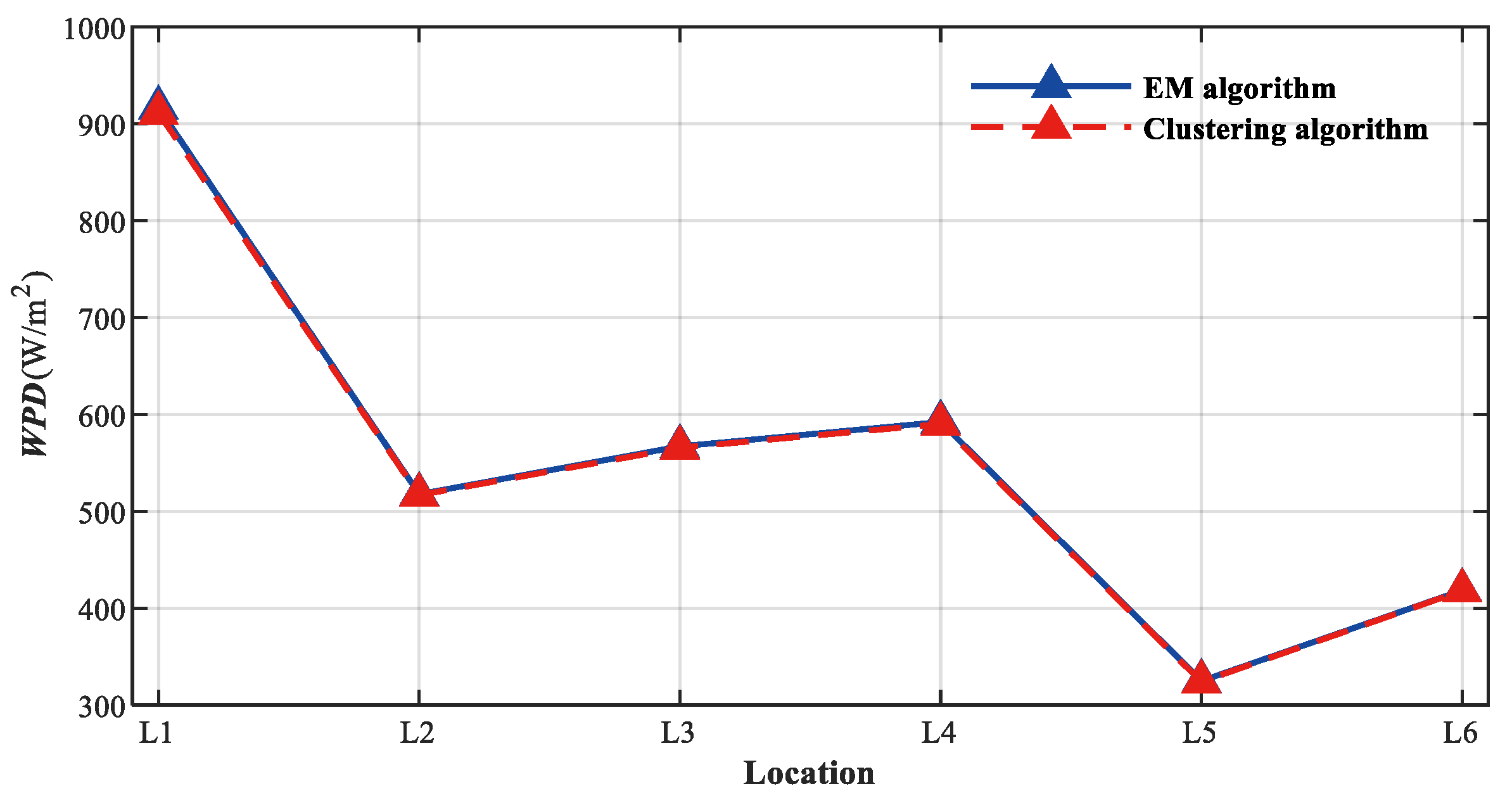
Both

Table 10. Wind power density (W/m²) across six selected locations.

Algorithm	L1	L2	L3	L4	L5	L6
EM algorithm	916.75	517.61	566.95	592.16	324.74	418.36
Clustering algorithm	911.36	516.61	565.49	590.04	323.89	417.92

and

Table 11. Annual energy production (GW·h) for the ASCD-8 turbine across six selected locations.

Algorithm	L1	L2	L3	L4	L5	L6
EM algorithm	42.12	28.99	31.19	31.94	21.68	26.13
Clustering algorithm	42.10	28.84	31.02	31.76	21.62	26.02

reveal that the WPD and AEP values determined by the clustering algorithm are in close proximity to those derived from the traditional EM algorithm.

This consistency, clearly depicted in Figure 15 and Figure 16, underscores the reliability and robustness of the proposed clustering algorithm in capturing and modeling wind energy characteristics. Specifically, discrepancies in WPD values across all six locations remain limited, with no variance surpassing 5.4 W/m². Similarly, the disparities in AEP values are found to be less than 0.2 GWh. Such minimal variations highlight the comparable efficiency demonstrated by both algorithms in estimating the energy potential from the wind speed and air density data.

While the EM algorithm has long served as a foundational tool in such assessments, the alignment of results between the two methods indicates that the clustering algorithm, introduced in this study, not only matches the performance of established methods but also presents an alternative computational approach for future wind energy research.

5. Discussion

In the presented research, the introduced clustering algorithm demonstrates a precision comparable to the well-established EM algorithm. However, it further offers distinct advantages that emphasize its enhanced adaptability in situations where the EM algorithm may encounter limitations.

A critical characteristic of the EM algorithm is its dependency on Q(ξ) to solve for the parameters of mixture models, described as:

$$Q\left(\xi \left|{\xi }^{\left(r-1\right)}\right.\right)={\displaystyle \sum _{i=1}^n{\displaystyle \sum _{j=1}^J\frac{{\omega }_j^{\left(r-1\right)}{f}_j\left(U_i\left|{\theta }_j^{\left(r-1\right)}\right.\right)}{{\displaystyle \sum _{k=1}^J{\omega }_k^{\left(r-1\right)}{f}_k\left(U_i\left|{\theta }_k^{\left(r-1\right)}\right.\right)}}\ln \left[{\omega }_j{f}_j\left(U_i\left|{\theta }_j\right.\right)\right]}}.$$

(23)

A pronounced challenge arises when dealing with complex probability density functions. As the complexity of these functions increases, the representation of Q(ξ) correspondingly intensifies, complicating the derivation of unknown parameters. The Q(ξ) of the distribution models presented in Equations (12)–(15) are given in Appendix A. By examining the contrast between the Q(ξ) of the one-dimensional probability density functions presented in Equations (A1) and (A2), and those of the two-dimensional probability density functions presented in Equations (A3) and (A4), an enhanced complexity associated with increased dimensionality is clearly discernible. Such increased complexity is especially pronounced when formulating three-dimensional joint distributions, for instance, involving random variables X, Y, and Z. When the vine copula is utilized to establish their joint probability density function, given by

$$\begin{array}{c}{f}_{XYZ}\left(x,y,z\right)={\displaystyle \sum _{j=1}^J{f}_{Xj}\left(x\right)\cdot f_{Yj}\left(y\right)\cdot f_{Zj}\left(z\right)\cdot c_{XZj}\left(F_{Xj}\left(x\right),F_{Zj}\left(z\right)\right)}\\ \hspace{1em}\hspace{1em}\hspace{1em}\hspace{1em}\hspace{1em}\hspace{1em}\cdot c_{YZj}\left(F_{Yj}\left(y\right),F_{Zj}\left(z\right)\right)\cdot c_{XY\left|Zj\right.}\left(F_{X\left|Zj\right.}\left(x\left|z\right.\right),F_{Y\left|Zj\right.}\left(y\left|z\right.\right)\right)\end{array},$$

(24)

the model incorporates three one-dimensional and three two-dimensional probability density functions. Given this complex structure, utilizing the EM algorithm for parameter estimation becomes significantly challenging.

Distinct from the EM algorithm, the clustering algorithm presented in this study offers a more direct approach. Instead of dealing with complex nonlinear equations, this technique transforms the challenge of mixture distribution models into multiple single-mode probability distributions. Consequently, when presented with an explicit form of the probability density function, the clustering algorithm effectively bypasses complexities associated with the likelihood function of mixture models. It utilizes data categorization to derive maximum likelihood estimates for individual data categories.

The experimental analysis and wind energy assessment conducted in China’s coastal region reveal the significant robustness and efficacy of the clustering algorithm. The results suggest that the performance of the clustering algorithm is not only comparable to that of the EM algorithm, but also consistently reliable across various data scenarios. In the experimental study, each subcategory’s data, obtained by the clustering algorithm for every case, can be well represented by a single probability distribution model, as depicted in Figure 4, Figure 5, Figure 6 and Figure 7. Additionally, the probability distribution parameters obtained for each subcategory in Table 3 closely match the predetermined parameters in Table 1. These findings suggest that the clustering algorithm introduced in this research, when classifying mixed data, ensures that the data of each subcategory satisfies homogeneity characteristics. Figure 17, Figure 18, Figure 19, Figure 20, Figure 21 and Figure 22 show the contour plots of the bivariate distribution for each subcategory of the mixed data from the coastal areas of China obtained through the clustering algorithm, while

Table 12. Statistical metrics for each subcategory of the mixed data across six locations.

Locations	Metrics	Component 1	Component 2	Component 3	Component 4	Component 5	Component 6	Component 7
L1	RMSE	0.0004	0.0002	0.0003	0.0003	0.0002	0.0002	0.0002
	R2	0.9672	0.9968	0.9567	0.9769	0.9924	0.9893	0.9948
L2	RMSE	0.0003	0.0002	0.0004	0.0005	0.0002	0.0001	—
	R2	0.9740	0.9948	0.9296	0.9164	0.9963	0.9977	—
L3	RMSE	0.0002	0.0003	0.0005	0.0006	0.0002	0.0002	0.0003
	R2	0.9680	0.9467	0.9413	0.9358	0.9870	0.9737	0.9645
L4	RMSE	0.0003	0.0002	0.0004	0.0001	0.0002	—	—
	R2	0.9321	0.9922	0.9243	0.9975	0.9957	—	—
L5	RMSE	0.0005	0.0004	0.0005	0.0004	0.0005	0.0005	0.0004
	R2	0.9658	0.9726	0.9678	0.9588	0.9718	0.9550	0.9522
L6	RMSE	0.0003	0.0006	0.0003	0.0002	0.0001	0.0006	—
	R2	0.9722	0.9398	0.9922	0.9842	0.9970	0.9283	—

lists the statistical error analysis results for these subcategories. The results indicate that the value of RMSE is small and the values of R² are all greater than 0.9, suggesting that each subcategory can be well fitted by a single-mode probability distribution model. Similar to the conclusions drawn from experimental research, studies on real data also demonstrate that the clustering algorithm proposed in this research not only has high accuracy but also ensures that each subcategory obtained from this classification satisfies homogeneity characteristics. Notably, in cases involving complex probability density functions, the clustering algorithm exhibits significant advantages, positioning itself as a compelling alternative to the EM algorithm.

While the proposed clustering algorithm presents promising accuracy and adaptability in wind energy research, it faces challenges related to computational demand, particularly with increasing sample sizes. Addressing this limitation is important for ensuring its scalability and wider applicability. One potential solution is the integration of parallel processing, utilizing the capabilities of modern multicore processors or specialized hardware such as graphics processing units. Given the divisibility of data clustering tasks, such an approach could significantly reduce computation times. Furthermore, the adoption of optimized data structures, such as trees or hash tables, can improve data efficiencies, thereby promoting quicker computations. In future research, these strategies will be thoroughly explored, with the aim of preserving the algorithmic accuracy while enhancing its computational efficiency, thus ensuring its viability in large-scale and real-time applications.

6. Conclusions

In the present study, a new clustering algorithm was proposed to estimate parameters in mixture distribution models. Carefully designed experiments were conducted to assess the algorithm’s performance in comparison to the established EM algorithm. Based on the experimental results, the precision of the suggested clustering algorithm was found to be comparable to the EM algorithm. Notably, when applied to wind energy assessment, a high degree of accuracy was exhibited by both algorithms, indicating their proficiency in predicting the probabilistic patterns for mixed data. Quantitative evaluations revealed the clustering algorithm’s robustness, with the root mean square error value being notably minimal and the coefficient of determination exceeding 0.9 for both experimental and real data analyses.

The EM algorithm often faces challenges with complex mixture multi-dimensional probability distributions, mainly due to its dependency on Q(ξ) to solve for the parameters. When dealing with complex probability density functions, the Q(ξ) can become exceedingly complex, making the EM algorithm less efficient. In contrast, the proposed clustering algorithm addresses these challenges by transforming mixture distributions into distinct single-mode probability distributions. This approach not only simplifies the estimation process but also broadens its applicability across various scenarios.

The investigation of wind resource assessment in China’s coastal regions highlighted the capabilities of the clustering algorithm. It accurately captures the multimodal structure of mixed wind data, enabling precise modeling of probabilistic distributions of wind speed and air density. The results further indicated that, for each subcategory derived from the clustering algorithm, the root mean square error values remained low and the coefficient of determination consistently exceeded 0.9. This suggests that each subcategory can be efficiently fitted by a single-mode probability distribution model, underscoring the algorithm’s ability to ensure subcategory obtained from classification homogeneity.

While the clustering algorithm demonstrates promising accuracy and adaptability in wind energy research, the computational demand, especially with larger datasets, is a challenge. To achieve scalability and wider application, future investigations should focus on addressing this limitation. One potential solution is applying parallel processing, utilizing modern multicore processors or specialized hardware like graphics processing units. Additionally, employing optimized data structures, like trees or hash tables, might improve data efficiency and speed up computations. Our future research will explore these optimization techniques, with the goal of enhancing both its efficiency and computational speed without compromising the precision of the results.