A Numerical Study of the Hydrodynamic Noise of Podded Propulsors Based on Proper Orthogonal Decomposition

Abstract

Podded propulsors have become a focal point of research in the field of marine propulsion in recent years due to their high efficiency, low noise, and excellent maneuverability. To investigate the acoustic characteristics induced by the flow field of podded propulsors, a high-precision unsteady numerical simulation was conducted using the Delayed Detached Eddy Simulation (DDES) coupled with Ffowcs Williams–Hawkings (FW-H) equations. Multiple spatial acoustic receiving arrays were employed, and analysis methods including Proper Orthogonal Decomposition (POD) and Fast Fourier Transform (FFT) were utilized to determine the spatial distribution of the acoustic field of the podded propulsor. The results show that the blade passing frequency and the shaft frequency consistently dominate as the primary characteristic frequencies. On the plane of the propeller disk, the distribution of sound pressure levels is uniform without distinct directivity. Across the space curved surface, approximately the first ten POD modes encompass 99.8% of the total energy, and their spatial distribution characteristics of sound pressure are closely related to the pod structure. Additionally, these modes exhibit characteristic frequencies such as the blade passing frequency and shaft frequency. The spatial distribution of sound pressure at a single frequency on the spatial surface corresponds well with the results obtained from the POD analysis.

1. Introduction

The podded propulsor, characterized by its high efficiency, low noise, and full maneuverability, has emerged as a prominent subject of research in the field of marine propulsion in recent years [1,2]. Research into podded propulsor technology is closely linked to the development of large high-speed vessels [3]. Atlar et al. [4] investigated several high-speed vessels equipped with podded propulsors and summarized the design and application of these propulsors in these vessels from the perspectives of environmental friendliness and efficiency.

In the early stages, research on podded propulsors primarily focused on their hydrodynamic performance and flow field structure. Examples include studies on the hydrodynamic performance of podded propulsors at various yaw angles [5], multi-component podded propulsors in straight flow [6], and extreme multi-load oblique flow conditions [7,8]. However, with the rapid advancement of high-tech vessels, higher demands have been placed on ship propulsion systems, with one of the most crucial aspects being hydrodynamic noise levels. Current research often employs numerical methods such as RANS [9,10,11,12], DES and its variations [13,14,15], and LES [16] coupled with the FW-H equation to simulate the hydrodynamic noise of isolate propellers. Results show that these various turbulence modeling methods can accurately capture the hydrodynamic performance and noise characteristics of podded propulsors. DES and LES methods can provide more detailed spatial flow field features, such as transient vortex structures, but require substantial computational resources. The hydrodynamic noise of isolate propellers has also been investigated experimentally. Felli M et al. [17] studied the hydrodynamic and hydroacoustic analysis of a marine propeller by using Tomographic Particle Image Velocimetry (Tomographic PIV). The hydrodynamic data of propeller wake flow were measured using PIV and the hydroacoustic data were calculated theoretically by using Powell’s vortex sound theory.

As for the complex flow structure analysis, Proper Orthogonal Decomposition (POD) is a data-driven analysis method that decomposes a random field into several modes that are temporally and spatially separated according to their energy content. It serves as a powerful tool for studying the spatiotemporal characteristics of complex random fields. Lumley [18] was the first to introduce this method into fluid mechanics research. The development of POD techniques has been comprehensively discussed by Taira et al. [19] to provide a detailed review of the application of POD in fluid mechanics. Magionesi F et al. [20] analysed the wake field past a marine propeller by using modal decomposition techniques, including POD and dynamic mode decomposition (DMD). Results showed that both POD and DMD could identify the temporal and spatial scales of complex propeller wake fields, so the modal decomposition technique is a useful method to investigate the flow field of a propeller.

In summary, the hydrodynamic performance and flow field structure of podded propulsors have been investigated sufficiently. However, as for the hydrodynamic noise, only the isolate propeller is considered in most research, while there is a lack of research on the overall hydrodynamic noise of the podded propulsor. Fortunately, the methods of investigation, including numerical simulation methods and POD, are universal. In the present paper, the Delayed Detached Eddy Simulation (DDES) method is used to obtain high precision numerical results. The POD and Fast Fourier Transform (FFT) method are utilized to analyze the data. Section 2 introduces the numerical implementation, and the verification and validation study are also carried out. In Section 3 and Section 4, results, discussions, and conclusions are presented.

2. Numerical Computational Methods

2.1. Numerical Theory

2.1.1. Turbulence Computational Governing Equations

In steady simulations, the Reynolds-Averaged Navier–Stokes (RANS) method is employed to obtain the initial flow field. In the current research, the Delayed Detached Eddy Simulation (DDES) method was used to simulate complex flow fields. The SST k-ω model was applied in the near-wall boundary layer region, while the Large Eddy Simulation (LES) method was utilized in regions away from the wall. The governing equations for the numerical model are given as follows [21]:

$$\frac{\partial k}{\partial t}+U_j\frac{\partial k}{\partial x_j}=\frac{1}{\rho }{P}_k-{\beta }^{\ast }k\omega \cdot F_{DDES}+\frac{1}{\rho }\frac{\partial }{\partial x_j}\left[\left(\mu +\frac{{\mu }_{\mathrm{t}}}{{\sigma }_k}\right)\frac{\partial k}{\partial x_j}\right]$$

(1)

$$\frac{\partial \omega }{\partial t}+U_j\frac{\partial \omega }{\partial x_j}=\frac{1}{\rho }{P}_{\omega }-\beta {\omega }^2+\frac{1}{\rho }\frac{\partial }{\partial x_j}\left[\left(\mu +\frac{{\mu }_{\mathrm{t}}}{{\sigma }_{\omega }}\right)\frac{\partial \omega }{\partial x_j}\right]+2\left(1-F_1\right)\rho {\sigma }_{\omega 2}\frac{1}{\omega }\frac{\partial k}{\partial x_j}\frac{\partial \omega }{\partial x_j}$$

(2)

where F_DDES is the switch function of the DDES method. When simulating the near-wall region, F_DDES was set to 1, and in regions far from the wall, it was set to 0. The DDES method employs the switch function to control the use of the SST model and LES model. This approach significantly reduces the computational time required for numerical simulations, while maintaining computational accuracy.

2.1.2. Acoustic Computational Governing Equations

Lighthill [22], by combining the Navier–Stokes equations and the acoustic wave equation, derived the fundamental equation for flow-induced noise:

$$\left(\frac{1}{c_0^2}\frac{{\partial }^2}{\partial t^2}-{\nabla }^2\right)\left[c_0^2\left(\rho -{\rho }_0\right)\right]=\frac{{\partial }^2{T}_{ij}}{\partial x_i\partial x_j}$$

(3)

$$T_{ij}=\rho u_i{u}_j+{\delta }_{ij}\left[\left(p-p_0\right)-c_0^2\left(\rho -{\rho }_0\right)\right]-{\sigma }_{ij}$$

(4)

where T_ij represents the Lighthill stress tensor. The Lighthill equation elucidates noise in turbulence but does not account for situations involving solid wall boundaries. Williams and Hawkings [23] extended this concept to moving solid boundaries using generalized function theory, leading to the formulation known as the FW-H equation:

$$\begin{array}{l}\left(\frac{1}{c_0^2}\frac{{\overline{\partial }}^2}{\partial t^2}-{\overline{\nabla }}^2\right)p^{\prime }\left(x,t\right)=\frac{\partial }{\partial t}\left\{\left[{\rho }_0{v}_0+\rho \left(u_n-v_n\right)\right]\delta \left(f\right)\right\}\\ \hspace{0.17em}\hspace{0.17em}\hspace{0.17em}\hspace{0.17em}\hspace{0.17em}\hspace{0.17em}\hspace{0.17em}\hspace{0.17em}\hspace{0.17em}\hspace{0.17em}\hspace{0.17em}\hspace{0.17em}\hspace{0.17em}\hspace{0.17em}-\frac{\partial }{\partial t}\left[\Delta P_{ij}{\widehat{n}}_j+\rho u_i\left(u_n-v_n\right)\delta \left(f\right)\right]\\ \hspace{0.17em}\hspace{0.17em}\hspace{0.17em}\hspace{0.17em}\hspace{0.17em}\hspace{0.17em}\hspace{0.17em}\hspace{0.17em}\hspace{0.17em}\hspace{0.17em}\hspace{0.17em}\hspace{0.17em}\hspace{0.17em}\hspace{0.17em}+\frac{{\overline{\partial }}^2}{\partial x_i\partial x_j}\left[T_{ij}H\left(f\right)\right]\end{array}$$

(5)

where $p^{\prime }$ represents the perturbation sound pressure, which is a function of time t and spatial coordinates x. Brentner et al. [24] introduced the Green’s function method and derived the time-domain integral formulation of the FW-H equation:

$$4\pi p_T{}^{\prime }\left(x,t\right)=\frac{\partial }{\partial t}{{\displaystyle {\int }_{f=0}\left[\frac{{\rho }_0{v}_n}{r\left|1-M_r\right|}\right]}}_{ret}dS$$

(6)

$$4\pi p_L{}^{\prime }\left(x,t\right)=\frac{1}{c_0}\frac{\partial }{\partial t}{{\displaystyle {\int }_{f=0}\left[\frac{l_r}{r\left|1-M_r\right|}\right]}}_{ret}dS+{{\displaystyle {\int }_{f=0}\left[\frac{l_r}{r^2\left|1-M_r\right|}\right]}}_{ret}dS$$

(7)

Equations (6) and (7) represent thickness noise and loading noise, respectively, and their sum yields the total sound pressure. It must be emphasized that the turbulence noise, known as quadrupole term, is neglected in the current research, since both the advance speed of the podded propulsor and the rotating speed of the propeller were much lower than the sound speed; that is, the Mach number was much less than 1 (even less than 0.1). In this case, the radiation efficiency of turbulent noise was almost zero and can be ignored. Correspondingly, if the working medium is air, such as in the case of airplanes, turbulent noise must be considered.

2.1.3. Proper Orthogonal Decomposition Theory

Within the flow field, consider a surface on which each grid node contains flow parameters such as velocity, pressure, vorticity, etc. These grid nodes also store data on how these flow parameters change over time. Let the number of grid nodes on this surface be n, and the duration of the observation be m time steps. In general, $n\gg m$. The flow parameters are denoted as q(ξ,t).

POD analysis involves decomposing q(ξ,t) into several spatially and temporally decoupled modes based on their energy content [19]:

$$q\left(\xi ,t\right)-\overline{q}\left(\xi \right)={\displaystyle \sum _i{a}_i\left(t\right){\varphi }_i\left(\xi \right)}$$

(8)

where $\overline{q}\left(\xi \right)$ is the time-averaged quantity of the flow field parameters. $a_i\left(t\right)$ represents the temporal coefficient, containing only time information. ${\varphi }_i\left(\xi \right)$ denotes the orthogonal basis functions, containing only spatial information. To determine the temporal coefficients and orthogonal basis functions, Singular Value Decomposition (SVD) is commonly employed.

Given that the left-hand side of Equation (8) is denoted as $x\left(\xi ,t\right)$, the data matrix is constructed as follows:

$$X=\left[\begin{array}{c}\begin{array}{cccc}x\left({\xi }_1,t_1\right)& x\left({\xi }_1,t_2\right)& \cdots & x\left({\xi }_1,t_m\right)\\ x\left({\xi }_2,t_1\right)& \ddots & \cdots & ⋮\\ ⋮& \cdots & \ddots & ⋮\\ x\left({\xi }_n,t_1\right)& \cdots & \cdots & x\left({\xi }_n,t_m\right)\end{array}\end{array}\right]\in {ℝ}^{n\times m}$$

(9)

Performing singular value decomposition on the data matrix X,

$$X=\Phi \Sigma {\Psi }^T$$

(10)

where $\Phi \in {ℝ}^{n\times n}$, $\Sigma \in {ℝ}^{n\times m}$, and $\Psi \in {ℝ}^{m\times m}$. $\Phi$ and $\Psi$ are the matrices of eigenvectors for $X{X}^T$ and $X^{T}X$, respectively. Only the main diagonal of these matrices contains non-zero values; the rest of the elements are zeros. The square of these non-zero values corresponds to the eigenvalues of $X{X}^T$ and $X^{T}X$. Since SVD arranges the eigenvalues in descending order, $\Phi$ effectively forms the matrix of orthogonal basis functions. The matrix of temporal coefficients can be determined through matrix operations:

$$A={\Phi }^{T}X\in {ℝ}^{n\times m}$$

(11)

In the preceding discussion, if q(ξ,t) is a scalar, SVD can be directly applied. However, if it is a vector, such as velocity, it is necessary to extract its components on the specified surface, construct data matrices for each component according to the same requirements, concatenate them, and then perform SVD. Similarly, acoustic field quantities can also undergo POD analysis. This paper primarily focuses on the analysis of sound pressure.

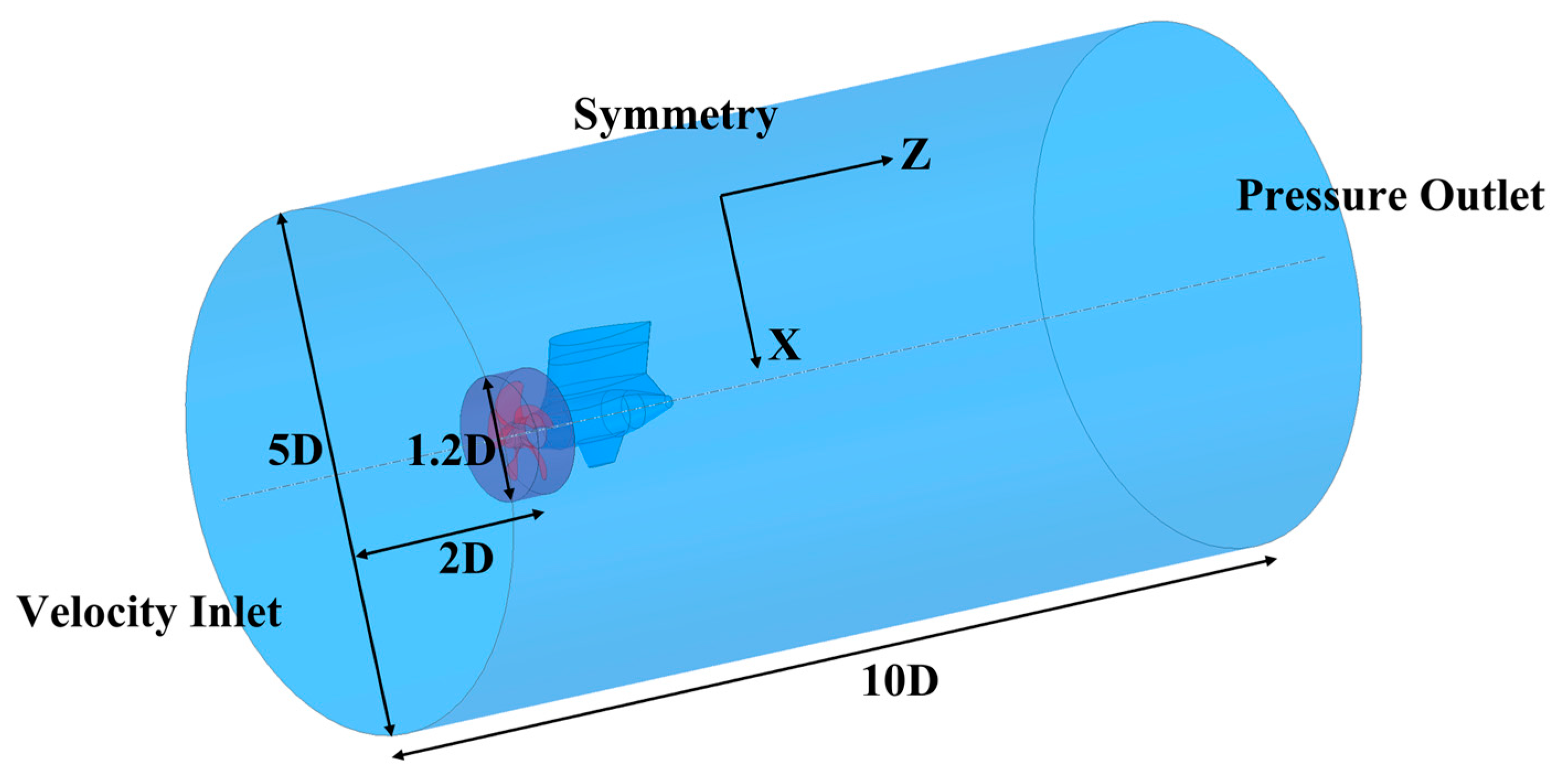
2.2. Mesh Generation

2.2.1. Computational Model

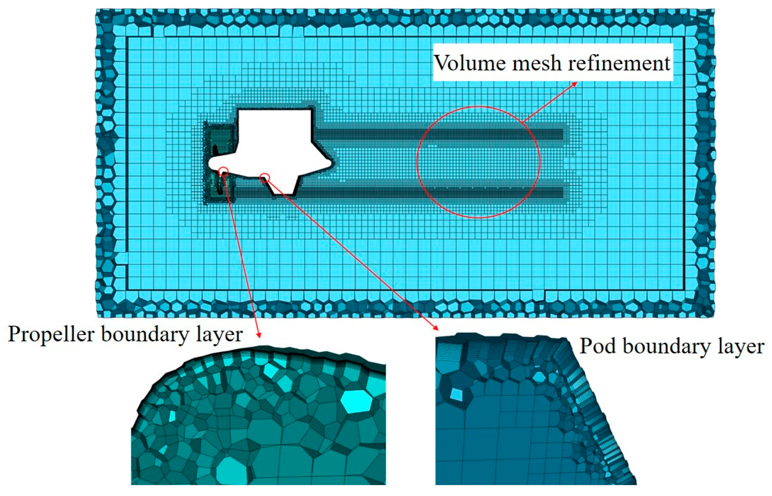
The computational domain for the podded propulsor is depicted in Figure 1, encompassing a stationary cylindrical domain and a rotating propeller domain. The parameters for the propeller and pod components are presented in

Table 1. Parameters of the podded propulsor.

Parameter	Value
Propeller Rotational Speed n (r/min)	1450
Propeller Diameter D (mm)	250
Number of Propeller Blades Z	5
Pod Heigh H (mm)	341.5
Pod Length L (mm)	503.2
Design Advance Coefficient J	0.8217

. The calculation formulas for the advance coefficient J, thrust coefficient K_T, and torque coefficient K_Q of the podded propulsor are as follows:

$$K_T=\frac{T}{\rho n^2{D}^4}$$

(12)

$$K_Q=\frac{Q}{\rho n^2{D}^5}$$

(13)

$$J=\frac{v}{nD}$$

(14)

where T, Q, ρ, n, D, and v, respectively, represent the thrust, torque, water density, propeller rotational speed, diameter, and inflow velocity of the propeller.

2.2.2. Mesh Grids

Considering the complexity of the podded propulsor model, which makes structured mesh generation challenging, the poly-hexcore technique based on ANSYS Fluent Meshing was chosen for unstructured mesh generation within the computational domain. As depicted in Figure 2, a polyhedral mesh was utilized near the wall surfaces, while a hexahedral mesh was applied in regions away from the walls. Between these two regions, transition layer grids transitioned from finer to coarser densities. To accurately capture pressure–time distributions on the propeller and pod surfaces, boundary layer refinement was applied to the model. A distribution map of wall y+ values was obtained through steady calculations, as shown in Figure 3. The results demonstrate that the overall average y+ value was around 10, with lower values near the propeller wall, satisfying the computational requirements of the DDES method.

2.3. Numerical Methods

The simulations were conducted using ANSYS Fluent for Computational Fluid Dynamics (CFD) and Computational Acoustics (CA). In the CFD calculations, the inlet and outlet were set as velocity inlet and pressure outlet, respectively. The exterior boundaries were defined as symmetry planes, imposing a normal flux of 0 for variables at the external boundaries to simulate far-field conditions in water. For the solution algorithm, bounded central differencing was chosen for momentum discretization, while second-order upwind schemes were used for pressure, turbulent kinetic energy, and specific dissipation rate discretization. An implicit second-order transient scheme was employed. The time step was set to 2.4414 × 10⁻⁴ s (1/4096 s) [25,26,27].

In the CA calculations, the far-field density was set to 1000 kg/m³, the far-field speed of sound was 1500 m/s, and the reference pressure in water was 1 × 10⁻⁶ Pa. The free stream velocity vector was set consistently with the velocity inlet. All surfaces of the podded propulsor were considered as sound source surfaces. With the mentioned settings, the simulation aimed to analyze the operational performance of the podded propulsor under the design condition (J = 0.8217).

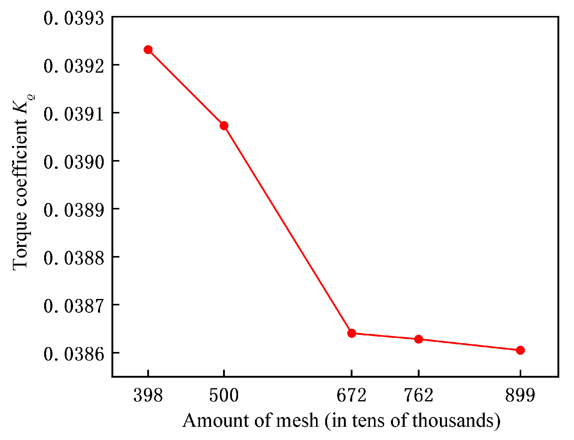
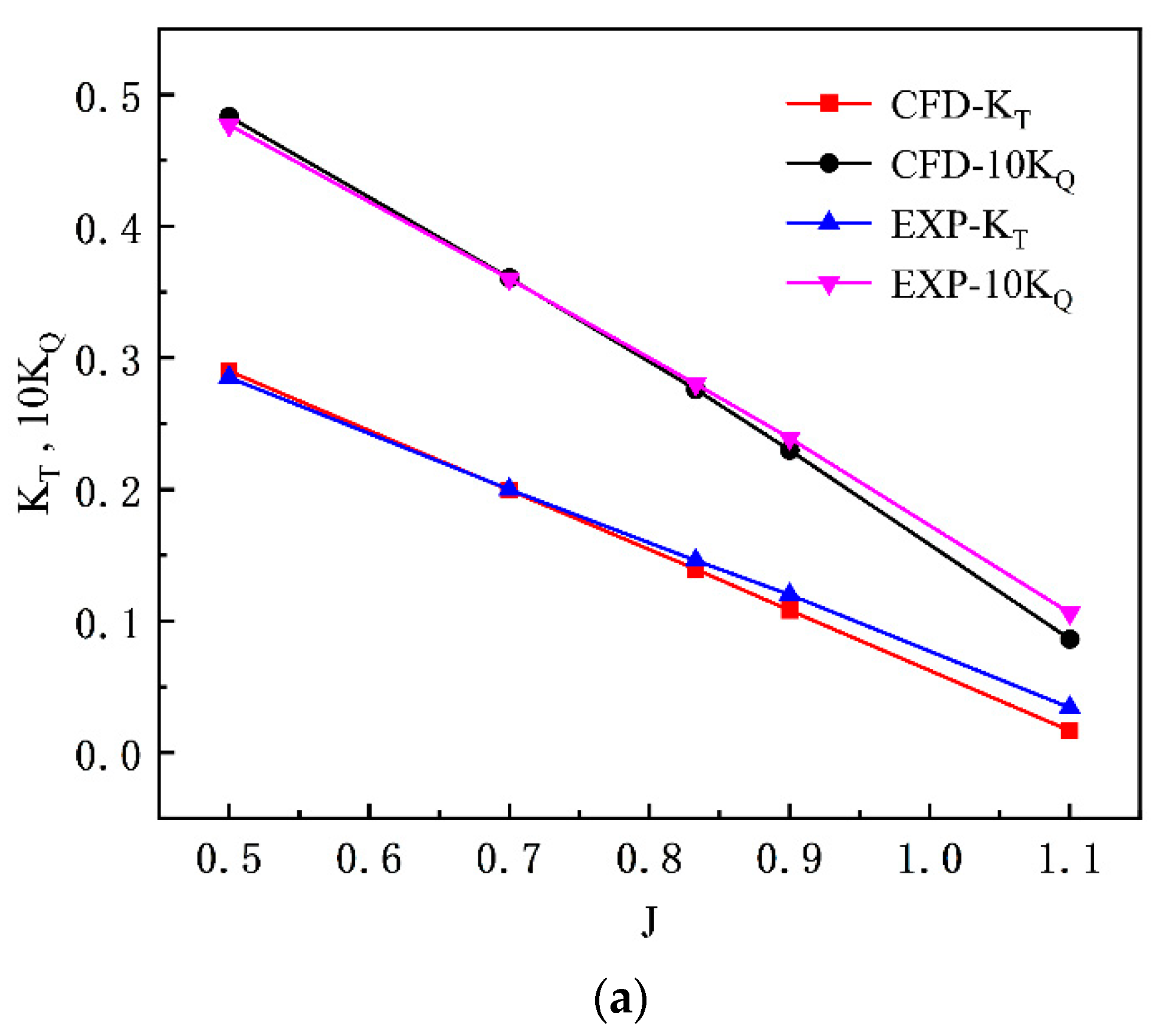
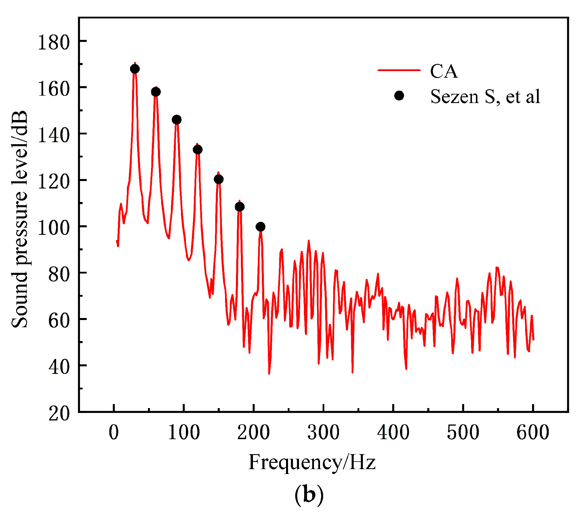
2.4. Numerical Method Verification and Validation

To begin with, several sets of grids were generated by adjusting the grid sizing parameters for mesh independence validation, as shown in Figure 4. The change in torque coefficient became relatively insignificant when the grid count reached around 7 million. Ultimately, grid schemes with 5.1 million cells for the rotating domain and 2.52 million cells for the stationary domain were selected.

As there are currently no available model experiment conditions, the validation of the numerical methods was performed using the standard propeller DTMB4119 [28]. The comparison of CFD results with hydrodynamic test data reported by JESSUP S D [28] is shown in Figure 5a. Under low advance coefficient conditions, there was a good agreement between numerical simulations and experimental data, whereas the error increased with the increase in the advance coefficient. The comparison of CA results with hydrodynamic noise data reported by SEZEN S et al. [23] is depicted in Figure 5b. The sound pressure levels at discrete frequencies, namely shaft frequency, blade passing frequency, and their harmonics, exhibited good agreement, with relative errors all less than 3%. The minimum absolute error was 0.31 dB and the maximum was 2.65 dB. This indicates that the numerical methods employed in this study exhibited high computational accuracy.

3. Results and Discussions

From the derivation of the FW-H equation, the source term for acoustic simulations was the water pressure–time data on the sound source surface. The presence of the podded body rendered the flow field distribution more complex, consequently resulting in intricate water pressure fluctuation patterns. The use of the DDES method allowed for the accurate acquisition of water pressure fluctuation patterns and their temporal data, thereby ensuring the accuracy of acoustic simulations. Additionally, during acoustic simulations, the entire surfaces of the propeller and pod were selected as sound source surfaces for computation.

3.1. Acoustic Field Distribution Characteristics on the Propeller Plane

On the propeller plane, twelve equidistant sound reception points were positioned at a radius of 155 mm, slightly outward in the rotating domain, resulting in a spacing of 30° between each pair of sound reception points. Sound pressure level calculations were performed on the acoustic pressure frequency domain data:

$$SPL=20\times {\log }_{10}\left(\frac{p_{amp}}{p_{ref}}\right)$$

(15)

where P_amp represents the sound pressure amplitude at the corresponding frequency after FFT, and P_ref is the reference sound pressure, with the value of 1 μ Pa in water. The sound pressure level at each sound reception point was extracted for the shaft frequency (24.17 Hz) and its 2nd to 21st harmonic frequencies. The contour plot of the harmonic frequencies is depicted in Figure 6. The energy distribution pattern of the sound pressure remained consistent among the twelve sound reception points, with the primary energy concentrated around the shaft frequency, blade passing frequency, and their harmonics. Sound pressure levels at other harmonic frequencies were relatively lower. As in Equation (15), sound pressure level is a logarithmic function. A 20 dB increase corresponds to a 10-fold increase in sound pressure. Therefore, the majority of sound pressure energy on the propeller plane was concentrated on a few characteristic frequencies, indicating minimal influence from other frequencies.

Standard deviations of sound pressure levels at twelve sound reception points for each harmonic frequency of the shaft frequency were computed and are depicted in Figure 7. The standard deviation of sound pressure at non-primary discrete frequencies was larger, with uneven circumferential energy distribution. Conversely, the standard deviation of sound pressure at primary discrete frequencies was smaller, resulting in a more even energy distribution. Given that the energy from primary discrete frequencies was dominant, it is hypothesized that sound waves radiating outward from the propeller plane exhibited little apparent directivity.

3.2. Acoustic Field Distribution Characteristics in the Spatial Domain

The distribution characteristics of the acoustic field in the spatial domain of the podded propulsor were explored by setting up an array of spatial sound reception points. As shown in Figure 8, spatial planes and spherical arrays were employed. The spherical array was generated with the z-axis (rotational axis) as its main axis, omitting singular points at the poles, composed of 49 × 51 sound reception points. The center of the sphere corresponded to the center of the propeller plane, with a radius of 500 mm, encompassing the entire podded propulsor. The planar array was parallel to the propeller plane, positioned at a z-axis coordinate of 451 mm, slightly aft of the pod, and had dimensions of 400 mm × 400 mm. It consisted of 51 × 51 sound reception points.

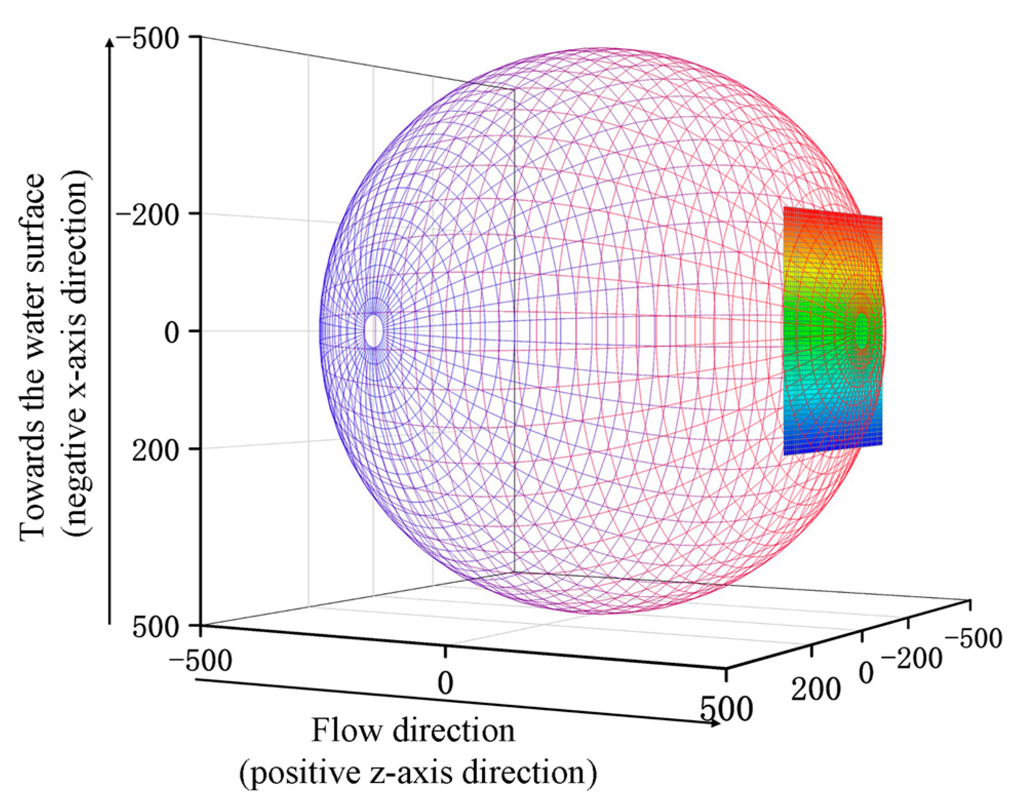
3.2.1. Spherical Sound Pressure Distribution

The sound pressure–time data obtained from the spherical sound reception point array was subjected to POD analysis. As shown in Figure 9, the cumulative energy percentage of the first 100 POD modes after decomposition is presented. The first 10 modes account for the vast majority of the energy, totaling to 99.8%. Consequently, the examination of the distribution of the initial few modes is sufficient.

Figure 10 illustrates the sound pressure distribution of the first four modes and the mean mode on the spherical surface. In the mean mode, the primary gradient change area of the sound pressure was located behind the podded propulsor. In this region close to the pod, the overall sound pressure level was significantly higher than in other areas, exhibiting some degree of directivity towards the water surface. The sound pressure distribution of the first and second modes was similar, and sound pressure gradually decreased from the positive y-axis to the negative y-axis and from the negative x-axis to the positive x-axis. However, fluctuations were observed near the tail of the pod, with the second mode even showing isolated low-pressure regions. The third and fourth mode sound pressure distributions resembled each other, with both exhibiting a symmetric distribution of high- and low-pressure regions with respect to the x-axis; however, the direction of gradient descent differed. As a comparison, Figure 11 shows the mean mode of an isolated propeller, in which all the conditions are the same as the podded propulsor, including the coordinate origin, geometric model of propeller, the relative position of the propeller, and all the numerical simulation settings. It can be clearly observed that the mean mode of the isolated propeller is a little different from that of the podded propulsor. In the circumferential direction, the mean mode of isolated propeller had no obvious directivity, while the mean mode of podded propulsor had an outstanding directivity. Apparently, this directivity is caused by the pod. Based on the comparison, it is stated that the characteristics of the mean mode and the sound pressure distribution of the first four modes are closely related to the pod, indicating a significant impact of the pod on the sound field distribution of the podded propulsor.

To understand the temporal characteristics of the sound field distribution on the spherical surface, FFT was applied to the time coefficients obtained from the POD decomposition. Figure 12 presents the frequency domain curves of time coefficients for the first four modes. The temporal characteristics of the dominant energy modes were consistent, with discrete characteristic frequencies of shaft and blade passing frequencies. However, the amplitude distribution varied among them. The amplitude at the shaft frequency was highest in the second mode and lowest in the fourth mode, while at the blade passing frequency, it was highest in the first mode and lowest in the second mode. The shaft frequency amplitudes of the first and fourth modes were smaller than their corresponding blade passing frequency amplitudes, whereas the second and third modes exhibited the opposite pattern. Overall, the shaft frequency amplitudes increased from the first mode to the second mode and then decreased, while the blade passing frequency amplitudes decreased from the first mode to the second mode and then increased, demonstrating complementary characteristics. Considering that modes beyond the fourth contribute very little energy, it can be inferred that the majority of the sound field energy on the spherical surface was concentrated around the shaft and blade passing frequencies. This analysis also reveals that while the POD analysis decomposes and ranks modes based on energy, different modes may correspond to multiple discrete characteristic frequencies in their time coefficients.

Performing FFT analysis on the sound pressure–time data obtained from the spherical surface allows for the analysis of sound pressure distribution at a single frequency. As shown in Figure 13, contour plots depict the sound pressure levels at the shaft and blade passing frequencies on the spherical surface. The perspective is from the negative z-axis, which corresponds to viewing from behind the propulsor towards the front. From the figure, there are distinct differences in the distribution characteristics of shaft and blade passing frequencies on the rear hemisphere. The low-pressure area at the shaft frequency exhibits an “∞” shape, while the low-pressure area at the blade passing frequency resembles an “8” shape. On the front hemisphere, in contrast to the POD results, the FFT results reveal certain regularities. Specifically, the sound pressure gradient gradually descends towards the negative z-axis, albeit with slight variations in the descent direction at the shaft and blade passing frequencies. Overall, the sound pressure distribution near the pod body exhibits distinct characteristics that vary with the characteristic frequencies, while the distribution becomes more consistent as one moves away from the pod body. The FFT results also underscore the significance of the pod body in influencing the sound pressure distribution.

3.2.2. Planar Sound Pressure Distribution

The sound pressure–time data obtained from the planar sound reception point array were subjected to POD analysis. As shown in Figure 14, the cumulative energy percentage of the first 100 POD modes after decomposition is presented. The first 12 modes account for the vast majority of the energy, totaling to 99.8%. Consequently, the examination of the distribution of the initial few modes is sufficient.

Figure 15 displays the sound pressure distribution of the first four modes and the mean mode on the plane. In the mean mode, the high-pressure area was located closest to the tail of the pod, which is the region nearest to the source plane and which exhibited the highest sound radiation intensity. The overall sound pressure distribution shows a gradient descent from the center outwards, with a certain degree of directionality (towards the water surface). This phenomenon is similar to the mean modal sound pressure distribution on the spherical surface and is primarily induced by the pylon.

The distribution of the first and second modes was similar, with concentrated areas of high and low pressure exhibiting symmetric patterns around the center of the plane. However, the gradient descent directions of sound pressure were opposite in these modes. The third mode had the lowest sound pressure values among the first four modes, and again it exhibited symmetric patterns of high and low pressure areas around the center of the plane. However, the gradient descent direction differed from the first and second modes. In the fourth mode, there were no concentrated areas of low pressure, and the overall trend was a decrease in pressure from the high-pressure area at the center of the plane towards the periphery. The characteristics of the first four modes and the mean mode were closely related to the pod body, and this conclusion aligned with the findings from the spherical sound pressure distribution.

To understand the temporal characteristics of the sound field distribution on the plane, the time coefficients obtained from the POD decomposition were subjected to FFT analysis. Figure 16 illustrates the frequency domain curves of the time coefficients for the first four modes. The dominant modes shared the same discrete characteristic frequencies, namely the blade passing frequency, shaft frequency, and a portion of its harmonics. However, their amplitudes differed. The amplitude at the shaft frequency was highest in the first mode, reaching its lowest in the fourth mode. The amplitude at the blade passing frequency was highest in the first mode and lowest in the third mode. The first, second, and third modes exhibited higher amplitudes at the shaft frequency compared to the blade passing frequency, while the fourth mode exhibited the opposite trend. Overall, the first mode provided the highest amplitude of time coefficients, whereas the fourth mode exhibited the lowest. The majority of the sound field energy on the plane was concentrated at the shaft frequency and blade passing frequency, which was consistent with the findings from the spherical sound field distribution.

The results of the POD analysis within the plane still do not completely isolate the characteristic frequencies. Performing FFT analysis on the sound pressure–time data obtained from the plane allows for the analysis of sound pressure distribution at a single frequency. As shown in Figure 17, contour plots of sound pressure level at shaft and blade passing frequencies on the plane are presented, with the perspective from the negative Z-axis, corresponding to a view from behind the propulsor towards the front. Sound pressure levels at shaft and blade passing frequencies exhibited high-pressure regions at the center of the plane, near the rear of the pod, indicating significant energy. However, the positions of low-pressure regions differed. The low-pressure area associated with the shaft frequency was situated to the right of the high-pressure region, showing some displacement. Conversely, the low-pressure region associated with the blade passing frequency was positioned above and below the high-pressure region, displaying a degree of symmetry. Overall, the characteristics of sound pressure level distribution at characteristic frequencies on the plane were similar to those observed on the spherical surface.

4. Conclusions

This study employed a coupled approach, integrating DDES with the FW-H equation to numerically simulate the flow and acoustic fields of a podded propulsor. Using a combined analysis of FFT and POD, the numerical results were analyzed, leading to the following conclusions:

(1)

On the propeller disc, the energy of sound pressure fluctuations was primarily concentrated at the shaft frequency, blade passing frequency, and their harmonics. However, the circumferential distribution of sound pressure levels was uniform, displaying no distinct directivity.

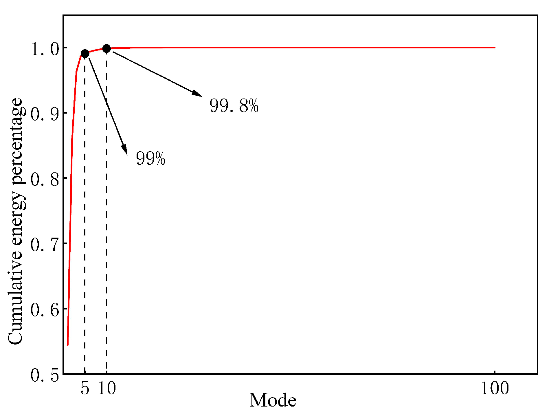
(2)

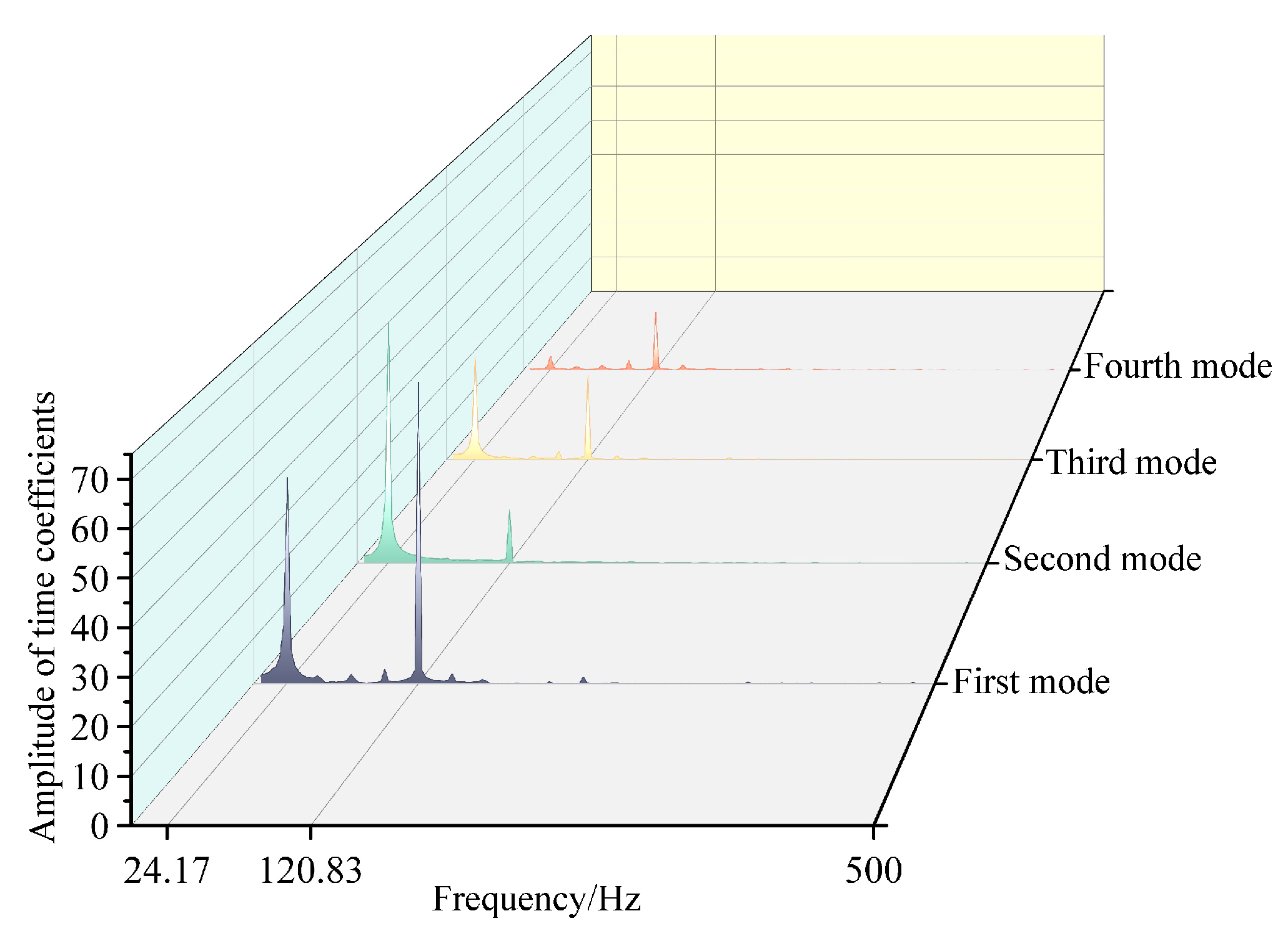
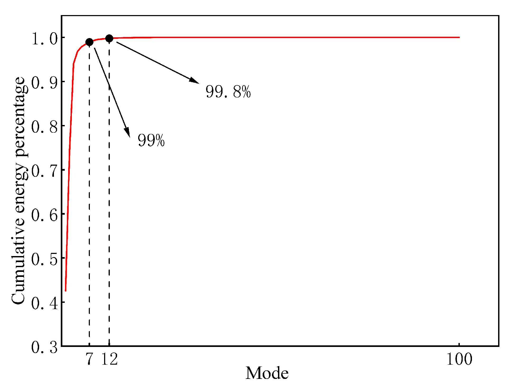
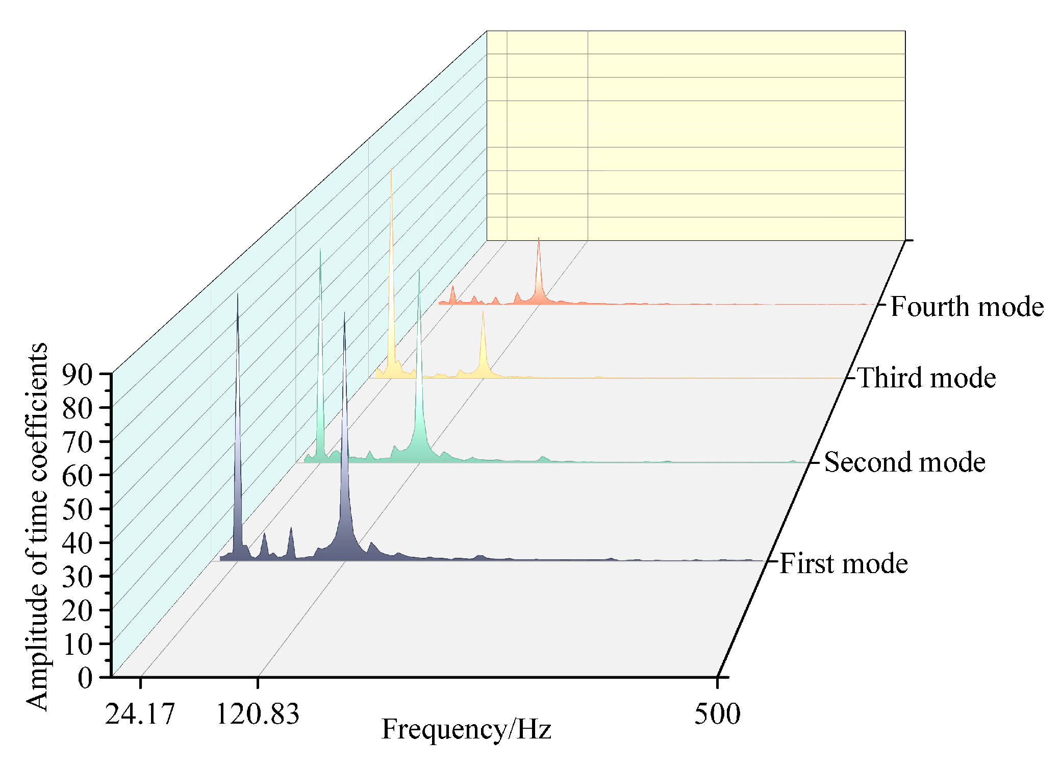
In the spatial spherical and planar surface, the first 10 and 12 POD modes, respectively, captured 99.8% of the energy. The first four modes exhibited sound pressure spatial distribution features closely tied to the pod, with their temporal features showing discrete frequencies primarily centered around the shaft and blade passing frequencies.

(3)

The FFT analysis of sound pressure revealed the single-frequency distribution characteristics on the spatial surfaces. The shaft and blade passing frequencies emerged as dominant frequency components, with distinct regions of high and low values. These regions correlated with the presence of the pod. Based on the results and discussions, it is evident that the POD method can identify the inherent distribution structure of hydrodynamic noise of podded propulsor. The POD method should have potential uses in podded propulsor design and its noise control strategies.

Under actual operating conditions, the podded propulsor operates within the wake field at the stern of the ship. This dynamic can result in non-uniform inflow to the propeller, potentially leading to efficiency reduction and higher noise levels. In addition, for many complex conditions, the podded propulsor may require complex steering operations, which can also lead to changes in the flow and sound fields. Future research will focus on coupling the podded propulsor with a realistic ship model and maneuverability to predict its noise characteristics.

References

1. Samoilescu, G.; Iorgulescu, D.; Mitrea, R.; Cizer, L.D. Propulsion Systems in Marine Navigation. In Proceedings of the International Conference Knowledge-Based Organization, Sibiu, Romania, 14–16 June 2018; Volume 24, pp. 78–82. [Google Scholar]
2. Nuchturee, C.; Li, T.; Xia, H. Energy efficiency of integrated electric propulsion for ships—A review. Renew. Sustain. Energy Rev. 2020, 134, 110145. [Google Scholar] [CrossRef]
3. Felli, M.; Falchi, M.; Dubbioso, G. Experimental approaches for the diagnostics of hydroacoustic problems in naval propulsion. Ocean. Eng. 2015, 106, 1–19. [Google Scholar] [CrossRef]
4. Atlar, M.; Woodwardm, D.; Besnier, F. FASTPOD Project: An Overall Summary Conclusions. In Proceedings of the 2nd International Conference on Technical Advances in Podded Propulsion (T-POD), Nantes, France, 2–3 October 2006; Newcastle University: Newcastle, UK, 2006. [Google Scholar]
5. Reza, S.; Hassan, G. Hydrodynamic analysis of puller and pusher of azimuthing podded drive at various yaw angles. J. Eng. Marit. Environ. 2014, 228, 55–69. [Google Scholar]
6. Antonio, S.; Timo, R.; Karl, R.; Tuomas, S. Numerical Investigation of Multi-Component Podded Propulsor Performance in Straight Flow. In Proceedings of the Fifth International Symposium on Marine Propulsors smp’17, Espoo, Finland, 12–15 June 2017. [Google Scholar]
7. Islam, M.F. Modeling techniques of puller podded propulsor in extreme conditions. J. Ship Res. 2017, 61, 230–255. [Google Scholar] [CrossRef]
8. Amini, H.; Sileo, L.; Steen, S. Numerical calculations of propeller shaft loads on azimuth propulsors in oblique inflow. J. Mar. Sci. Technol. 2012, 17, 403–421. [Google Scholar] [CrossRef]
9. Islam, M.; Jahra, F.; Ryan, R.; Hedd, L. Hydrodynamics of Podded Propulsors with Highly Loaded Propellers and in Extreme Azimuthing Conditions. In Proceedings of the International Conference on Offshore Mechanics and Arctic Engineering, St John’s, NL, Canada, 31 May 2015; p. V011T12A027. [Google Scholar]
10. Mohsen, G.; Hassanm, G.; Jalalm, M. Calculation of sound pressure level of marine propeller in low frequency. J. Low Freq. Noise Vib. Act. Control. 2018, 31, 60–73. [Google Scholar]
11. Guo, C.; Xu, P.; Wang, L.; Luo, W. Hydrodynamic performance analysis of podded propulsor under ice blockage condition. J. Huazhong Univ. Sci. Technol. 2018, 46, 41–46. [Google Scholar]
12. Nie, Y.; Ouyang, W.; Li, G.; Zhang, C.; Zhou, X. Simulation study on hydrodynamic performance of podded propulsor for curise ship. Chin. J. Ship Res. 2022, 17, 170–177+195. [Google Scholar]
13. Ville, M.; Viitanen, A.H.; Tuomas, S.; Siikonen, T. DDES of Wetted and Cavitating Marine Propeller for CHA Underwater Noise Assessment. J. Mar. Sci. Eng. 2018, 6, 56. [Google Scholar]
14. Pan, Y.; Zhang, H. Numerical Hydro-Acoustic Prediction of Marine Propeller Noise. Shanghai Jiaotong Univ. 2010, 15, 707–712. [Google Scholar] [CrossRef]
15. Mei, Z.; Gao, B.; Zhang, N.; Lai, Y.; Li, G. Numerical Study on the Unsteady Flow Field Characteristics of a Podded Propulsor Based on DDES Method. Energies 2022, 15, 9117. [Google Scholar] [CrossRef]
16. Lidtke, A.K.; Humphrey, V.F.; Turnock, S.R. Feasibility study into a computational approach for marine propeller noise and cavitation modeling. Ocean. Eng. 2016, 120, 152–159. [Google Scholar] [CrossRef]
17. Felli, M.; Falchi, M.; Dubbioso, G. Tomographic-PIV survey of the near-field hydrodynamic and hydroacoustic characteristics of a marine propeller. J. Ship Res. 2015, 59, 201–208. [Google Scholar] [CrossRef]
18. Lumley, J.L. The structure of inhomogeneous turbulent flows. In Atmospheric Turbulence and Radio Wave Propagation; Scientific Research: Moscow, Russia, 1967; pp. 166–178. [Google Scholar]
19. Taira, K.; Brunton, S.L.; Dawson, S.T.M.; Rowley, C.W.; Colonius, T.; McKeon, B.J.; Schmidt, O.T.; Gordeyev, S.; Theofilis, V.; Ukeiley, L.S. Modal analysis of fluid flows: An overview. AIAA J. 2017, 55, 4013–4041. [Google Scholar] [CrossRef]
20. Magionesi, F.; Dubbioso, G.; Muscari, R.; Di Mascio, A. Modal analysis of the wake past a marine propeller. J. Fluid Mech. 2018, 855, 469–502. [Google Scholar] [CrossRef]
21. Menter, F.R.; Kuntz, M.; Langtry, R. Ten years of industrial experience with the SST turbulence model. Turbul. Heat Mass Transf. 2003, 4, 625–632. [Google Scholar]
22. Lighthill, M.J. On sound generated aerodynamically I. General theory. In Proceedings of the Royal Society of London. Series A. Mathematical and Physical Sciences; Royal Society: London, UK, 1952; Volume 211, pp. 564–587. [Google Scholar]
23. Williams, J.F.; Hawkings, D.L. Sound generation by turbulence and surfaces in arbitrary motion. In Philosophical Transactions of the Royal Society of London. Series A, Mathematical and Physical Sciences; Royal Society: London, UK, 1969; Volume 264, pp. 321–342. [Google Scholar]
24. Brentner, K.S.; Farassat, F. Modeling aerodynamically generated sound of helicopter rotors. Prog. Aerosp. Sci. 2003, 39, 83–120. [Google Scholar] [CrossRef]
25. Sezen, S.; Kinaci, O.K. Incompressible flow assumption in hydroacoustic predictions of marine propellers. Ocean. Eng. 2019, 186, 106138. [Google Scholar] [CrossRef]
26. Li, D.; Zhang, N.; Jiang, J.; Gao, B.; Alubokin, A.A.; Zhou, W.; Shi, J. Numerical investigation on the unsteady vortical structure and pressure pulsations of a centrifugal pump with the vaned diffuser. Int. J. Heat Fluid Flow 2022, 98, 109050. [Google Scholar] [CrossRef]
27. Zhang, N.; Gao, B.; Ni, D.; Liu, X. Coherence analysis to detect unsteady rotating stall phenomenon based on pressure pulsation signals of a centrifugal pump. Mech. Syst. Signal Process. 2021, 148, 107161. [Google Scholar] [CrossRef]
28. Jessups, D. An Experimental Investigation of Viscous Aspects of Propeller Blade Flow; The Catholic University of America: Washington, DC, USA, 1989. [Google Scholar]
Figure 1. Computational domain of the podded propulsor model.
Jmse 11 02054 g001
Figure 2. Mesh structure.
Jmse 11 02054 g002
Figure 3. Wall y+ value distribution.
Jmse 11 02054 g003
Figure 4. Mesh independence verification.
Jmse 11 02054 g004
Figure 5. Numerical method validation [23]: (a) CFD validation. (b) CA validation.
Jmse 11 02054 g005aJmse 11 02054 g005b
Figure 6. Sound pressure level of shaft frequency harmonic.
Jmse 11 02054 g006
Figure 7. Standard deviation of harmonic frequencies.
Jmse 11 02054 g007
Figure 8. Spatial sound reception point arrays.
Jmse 11 02054 g008
Figure 9. Cumulative energy percentage of POD modes from a spherical array.
Jmse 11 02054 g009
Figure 10. Sound pressure distribution of POD modes on the spherical surface. (a) Mean mode. (b) First mode. (c) Second mode. (d) Third mode. (e) Fourth mode.
Jmse 11 02054 g010
Figure 11. Sound pressure distribution of POD mean mode on the spherical surface.
Jmse 11 02054 g011
Figure 12. Waterfall plot of frequency domain time coefficients for POD modes on the spherical surface.
Jmse 11 02054 g012
Figure 13. Sound pressure level projection on the spherical surface. (a) Shaft frequency in the front hemisphere. (b) Shaft frequency in the rear hemisphere. (c) Blade passing frequency in the front hemisphere. (d) Blade passing frequency in the rear hemisphere.
Jmse 11 02054 g013
Figure 14. Cumulative energy percentage of POD modes from planar array.
Jmse 11 02054 g014
Figure 15. Sound pressure distribution of POD modes on the plane. (a) Mean mode. (b) First mode. (c) Second mode. (d) Third mode. (e) Fourth mode.
Jmse 11 02054 g015aJmse 11 02054 g015b
Figure 16. Waterfall plot of frequency domain time coefficients for POD modes on the plane.
Jmse 11 02054 g016
Figure 17. Contour plot of sound pressure level on the plane. (a) Shaft frequency. (b) Blade passing frequency.
Jmse 11 02054 g017