Implications of Reynolds Averaging for Reactive Tracers in Turbulent Flows

Abstract

RANS simulations have been broadly used to investigate turbulence in the oceans and atmosphere. Within these environments there are a multitude of tracers undergoing reactions (e.g., phytoplankton growth, chemical reactions). The distribution of these reactive tracers is strongly influenced by turbulent mixing. With a 50 member ensemble of two-dimensional Rayleigh–Taylor-induced turbulent mixing, we show that the dynamics of a reactive tracer growing according to Fisher’s equation are poorly captured by the ensemble mean. A fluctuation-dependent sink introduced by Reynolds averaging Fisher’s equation transfers tracer concentration from the mean to the fluctuations. We compare the dynamics of the reactive tracer with those of a passive tracer. The reaction increases the reactive tracer’s concentration thereby increasing Fickian diffusion and allowing the reactive tracer to diffuse into turbulent structures that the passive tracer cannot reach. A positive feedback between turbulent mixing and fluctuation growth is identified. We show that eddy viscosity and diffusivity parameterizations fail to capture the bulk trends of the system and identify a need for negative eddy diffusivities. One must, therefore, be cautious when interpreting RANS results for reactive tracers.

1. Introduction

The ocean exhibits motions over an amazing range of scales, from the 1000 km scale of ocean gyres, to the sub-centimeter scale on which viscous dissipation removes energy from the system. Modern oceanography relies on field measurements, remote sensing, and, increasingly, numerical simulations of ocean processes. All of these have their own established methodology, yet all fail to provide a complete description of the ocean. The influence of physical processes on biogeochemical ocean dynamics is an active area of research in which numerical models play an important role as investigative and predictive tools [1,2,3,4,5]. The performance of a numerical model is limited by the underlying numerical method and model resolution. These are, in turn, limited by the availability of computational resources. Ocean modelers must thus make choices as to which processes to resolve, which to parameterize, and at times, even which to ignore.

The Regional Ocean Modeling System (ROMS) is a popular tool for conducting regional (on the order of tens of kilometers) simulations due to its flexibility and stable numerical methodology. It has a topography-following coordinate system in the vertical, an implicit free-surface, and can be run as a coupled physical–biogeochemical model [6]. ROMS is a split-explicit model, meaning fast and slow dynamics are split into sub-problems. If non-dissipative time-stepping is used for both, the model becomes unstable [7,8]. Time-stepping algorithms with forward–backward feedback are used to enhance the internal stability of the model [9]. In addition to the numerical diffusivity introduced by the time-stepping method, ROMS treats horizontal and vertical diffusion differently, and has a number of options for parameterizing vertical mixing [7,10] all of which are, by nature, dissipative [11]. While not strictly necessary, the majority of regional modeling studies invoke the hydrostatic approximation, meaning some processes (e.g., density overturns) are inherently excluded from consideration. Example use cases for ROMS include the Atlantic Canada Model ($O(10$ km) horizontal resolution and 30 vertical levels) [12], the Coupled Ocean–Atmosphere–Wave–Sediment Transport modeling system (4.7–9.0 km horizontal resolution, 50 vertical layers spanning 8 km) [13], and studies of storm-induced circulation and hydrography changes in tropical regions (6 km resolution) [14]. The diversity of studies that use ROMS indicates the importance of model flexibility and adaptability.

ROMS and similar models effectively solve the Reynolds-averaged Navier–Stokes (RANS) equations. Reynolds averaging is a commonly applied procedure in the study of turbulent flows [15]. It consists of decomposing a physical quantity into its ensemble mean and fluctuating parts. The procedure will be illustrated in Section 2.1.1. The appeal of RANS simulations comes from the reduced computational cost of simulating only the mean state of a system as opposed to running an ensemble of simulations. However, ensemble averaging the Navier–Stokes momentum equation introduces the Reynolds stress tensor, which poses a closure problem [15]. Despite the challenge of parameterizing the Reynolds stresses, RANS is a popular method for simulating naturally occurring turbulent flows, which are ubiquitous in the oceans and atmosphere and are known to cause strong mixing [16,17]. Turbulent flows are characterized by large, irregular variations in space and time, making their details unpredictable [18]. These variations often manifest in the form of vortices or filaments. For a discussion of several classes of models, as well as popular modeling techniques and closures when using RANS for turbulence modeling, see [19]. For a review of the uncertainty in RANS models, see [20].

Eddy viscosity models are the most common choice for parameterizing Reynolds stresses, largely owing to their relative simplicity. These models assume that the Reynolds stress tensor is aligned with the mean strain tensor, allowing the Reynolds stress term to be related to the ensemble mean velocity field [15,18]. In practice, the Reynolds stress terms in the RANS momentum equation are replaced by simply introducing additional viscosity into the system [15]. These models assume that the local gradient of the mean velocity field dictates the direction of flux. However, if the advection in a turbulent flow is strong enough, the large eddies that emerge may dominate and cause the flux to be oriented against the gradient [18], making the eddy viscosity assumption invalid. In particular, there are cases in which the eddy viscosity becomes negative and the model breaks down because anti-diffusion is mathematically ill-posed [21]. There are numerous eddy viscosity models which fall under the broad categories of mixing-length models, one-equation models, and two-equation models among others [22]. Other eddy viscosity models have been developed for large eddy simulations, such as the Lilly–Smagorinsky model [23].

Analogously, the Reynolds fluxes that emerge from Reynolds averaging scalar transport equations are often modeled by eddy diffusivities. Eddy diffusivities have been estimated for passive tracers with satellite observations and found to be strongly space and time dependent [24]. In the upper 2000 m of the oceans, horizontal eddy diffusivities on a 300 km scale range between ${10}^2$ m${}^2$/s and ${10}^4$ m${}^2$/s [25,26,27]. The expression used to calculate the eddy diffusivity inevitably affects the estimate. If one were to consider the suppression of mixing by mean currents, then the spatial distribution and magnitude of the eddy diffusivities would differ dramatically [28] compared to estimations that simply use mixing length theory [29]. Evidence has suggested that in stratified fluids, the ocean being a prime example, eddy diffusivity should be modeled as a decreasing function of buoyancy frequency [30].

Eddy mixing is also strongly dependent on the tracer being considered [31]. Active tracers may require counter-gradient fluxes rather than down-gradient fluxes, resulting in negative eddy diffusivities [32]. For instance, double diffusion displays a counter-gradient density flux, while turbulence transports density down-gradient [33]. Though some methods for determining eddy diffusivities and transport characteristics have shown indistinguishable performance when used for passive or active tracers [34], this cannot be the case for reactive tracers, the dynamics of which are inevitably more complicated. Several methods for modeling the eddy diffusivity of a reactive tracer have been presented in the literature. Ensembles of Lagrangian particle trajectories have been used to determine a time-dependent diffusion function that yields the effective eddy diffusivity when evaluated at the reaction timescale [35]. The gradient-diffusion hypothesis has been examined by regressing true eddy fluxes onto tracer gradients to determine an effective eddy diffusivity [36]. It was shown to perform more poorly for reactive versus non-reactive tracers, with the specifics depending on the model parameters.

The effect of turbulence on the reaction dynamics of nutrient phytoplankton zooplankton (NPZ) models has been considered through several different lenses [35,37,38]. NPZ models are almost always expressed in terms of advection–diffusion–reaction (ADR) equations. Complications arise from the impact of turbulence on the spatial distribution of a reactive tracer possibly affecting the reaction rate [38]. Further, eddy reaction terms, defined as covariances of tracer fluctuations, are introduced when the reaction function is Reynolds-averaged. Eddy reactions are inevitably strongly reaction-dependent and have been shown to be sensitive to seasonality, location, and spatial scales for some NPZ models [39].

In addition to being a popular tool for examining oceanic ecosystems, RANS has been used to model reactive tracers in the contexts of water disinfection [40,41,42], the spread of air pollutants [43], and combustion [44]. In this paper, we take a step back and consider a simple system in which a reactive tracer grows according to Fisher’s equation within a Rayleigh–Taylor (RT) flow. So called “toy” flows, for which velocities are specified instead of solved for, have proven to be a useful tool for conducting initial investigations into the effect of turbulence on phytoplankton [37]. Velocities are often chosen so that the flow field is composed of convective cells of multiple scales that oscillate in space [37,45]. The cells are intended to represent flows due to thermal convection and the range of scales is introduced to mimic turbulence. They are thought to be especially useful when considering under-ice convection, as ice cover eliminates all wind-driven turbulent mixing [45,46]. However, this method fails to capture the cascade of energy between scales in turbulent flows, nor does it account for the dissipation of turbulent kinetic energy, making it a poor representation of ocean dynamics.

We choose Rayleigh–Taylor (RT) instability-induced turbulent mixing as a non-trivial, yet well studied illustrative example. From figure 2 in [47], it is apparent that RT flows are not cell-like and evolve into turbulent states. For a discussion of several turbulence model choices for RT instabilities, see [48,49]. RT instabilities have some memory of the spatial structure of their initial conditions when we consider large-scale effects, but the smaller-scale internal structure makes the mixing unpredictable [50]. Two-dimensional simulations fail to capture the internal structure of the flow and, thus, cannot describe the turbulent mixing that would be seen in three dimensions [47,50,51]. For the purpose of constructing an illustrative example, however, two-dimensional simulations will suffice.

To the best of our knowledge, there does not exist any literature analyzing the ability of a Reynolds average to capture the dynamics of a reactive tracer in a turbulent flow. Further, the existing literature has not examined the mechanisms that describe how turbulence might affect reactive or passive tracers differently. The simplicity of the numerical experiment reported herein allows us to illustrate the differences between passive and reactive tracer fields evolving under turbulence. In particular, we illustrate that the evolution of a reactive tracer is poorly captured by the ensemble mean and that eddy diffusivity parameterizations are not appropriate for our simulations. The remainder of this paper is structured as follows. In Section 2, we present the governing equations and demonstrate how Reynolds averaging can be applied to ADR equations. The results from an ensemble of 50 simulations are presented in Section 2.2 to illustrate differences in the effects of turbulent mixing on a passive tracer versus a reactive tracer growing according to Fisher’s equation. The limitations of using RANS simulations to model reactive tracers will be discussed in Section 5.

2. Methods

2.1. Governing Equations

Consider the following set of partial differential equations:

$$\begin{array}{}\mathrm{(1)}& \hfill & {\overrightarrow{u}}_t+\nabla ·\left({\overrightarrow{u}}^T\overrightarrow{u}\right)=-\frac{1}{{\rho }_0}\nabla p+\frac{{\rho }_E}{{\rho }_0}\overrightarrow{g}+\nu {\nabla }^2\overrightarrow{u},\hfill \mathrm{(2)}& \hfill & {\theta }_t+\nabla ·\left(\overrightarrow{u}\theta \right)=\kappa {\nabla }^2\theta +F\left(\theta \right).\hfill \end{array}$$

We report the excess density, defined as a departure from the reference density

$$\begin{array}{c}\hfill {\rho }_E=\rho (\overrightarrow{x},t)-{\rho }_0.\end{array}$$

(3)

SPINS (spectral parallel incompressible Navier–Stokes solver) [52] will be the model used herein. The excess density is evolved through an ADR equation, like that for $\theta$, but without a source term.

In Equation (1), the conservation of mass, $\nabla ·\overrightarrow{u}=0$ has been used to rewrite $\overrightarrow{u}·\nabla \overrightarrow{u}$ as $\nabla ·\left({\overrightarrow{u}}^T\overrightarrow{u}\right)$. The second equation is an ADR equation describing the evolution of a scalar tracer undergoing a reaction given by the function $F\left(\theta \right)$. A reactive tracer has a nonzero reaction term, but we assume that it does not affect the properties of the fluid. Reactive tracers are an important component in biophysical models describing ecosystem dynamics, which generally include components evolved by growth and interaction terms [2,3,4,5,53].

2.1.1. Reynolds Averaging

We will use the overbar notation to denote Reynolds averaging. We decompose the velocity field into a slowly varying mean part, $\overrightarrow{U}$, and a rapidly fluctuating part, ${\overrightarrow{u}}^{\prime }$, so that $\overrightarrow{u}=\overrightarrow{U}+{\overrightarrow{u}}^{\prime }$ with $\overline{\overrightarrow{U}}=\overrightarrow{U}$ and $\overline{{\overrightarrow{u}}^{\prime }}=0$. Similarly, for the pressure and excess density we have $p=P+p^{\prime }$ and ${\rho }_E={\mathcal{P}}_E+{\rho }_E^{\prime }$. The Reynolds-averaged momentum equation is

$$\begin{array}{cc}\hfill {\overrightarrow{U}}_t+\nabla ·\left({\overrightarrow{U}}^T\overrightarrow{U}\right)& \hfill =-\frac{1}{{\rho }_0}\nabla P+\frac{{\mathcal{P}}_E}{{\rho }_0}\overrightarrow{g}+\nu {\nabla }^2\overrightarrow{U}-\nabla ·\overline{{\overrightarrow{u}}^{\prime T}{\overrightarrow{u}}^{\prime }}.\hfill \end{array}$$

(4)

The Reynolds stress tensor describes the effects of the fluctuations on the mean flow and is defined as $R_{ij}=\overline{u_i^{\prime }{u}_j^{\prime }}$.

The procedure can be applied to Equation (2) by decomposing the tracer field in the same way: $\theta =\Theta +{\theta }^{\prime }$. The Reynolds-averaged ADR equation is

$$\begin{array}{cc}\hfill {\Theta }_t+\nabla ·(\overrightarrow{U}\Theta )& \hfill =\kappa {\nabla }^2\Theta +\overline{F(\Theta +{\theta }^{\prime })}-\nabla ·\overline{{\overrightarrow{u}}^{\prime }{\theta }^{\prime }},\hfill \end{array}$$

(5)

where $\overline{{\overrightarrow{u}}^{\prime }{\theta }^{\prime }}$ is the eddy flux representing the transport of tracer fluctuations by fluctuations in the velocity field. The treatment of the $\overline{F(\Theta +{\theta }^{\prime })}$ term will be considered in Section 2.1.2.

2.1.2. Reynolds Averaging $F\left(\theta \right)$

Fisher’s equation, $F\left(\theta \right)=\theta (1-\theta )$, will be used as an illustrative example, but the procedure presented herein can be used to treat any reaction term expressed as (or approximated by) a polynomial. Fisher’s equation provides a simple, non-linear reaction function and has been used to describe population growth. Further, we know the differential equation $d\theta /dt=\theta (1-\theta )$ has an unstable equilibrium at 0 and a stable equilibrium at $\theta =1$. Therefore, in the absence of advection, the tracer would simply grow towards a value of 1 everywhere in the domain.

Consider a polynomial reaction function of degree N. We want to rewrite $\overline{{\theta }^n}$ in a way that allows us to separate the effects due to the mean tracer field, those due to fluctuations, and those due to cross-interactions of the two. By substituting $\theta =\Theta +{\theta }^{\prime }$, the reactions can be binned as follows

$$\begin{array}{}\mathrm{(6)}& \hfill \overline{{\theta }^n}& =\overline{{(\Theta +{\theta }^{\prime })}^n}\hfill \mathrm{(7)}& & =\sum _{{\alpha }_1+{\alpha }_2=n;{\alpha }_1,{\alpha }_2\ge 0}\left(\genfrac{}{}{0pt}{}{n}{{\alpha }_1,{\alpha }_2}\right)\overline{{\Theta }^{{\alpha }_1}{\left({\theta }^{\prime }\right)}^{{\alpha }_2}}\hfill \mathrm{(8)}& & ={\Theta }^n+\underset{I_n}{\underbrace{\sum _{{\alpha }_1+{\alpha }_2=n;{\alpha }_1>0{\alpha }_2>1}\left(\genfrac{}{}{0pt}{}{n}{{\alpha }_1,{\alpha }_2}\right){\Theta }^{{\alpha }_1}\overline{{\left({\theta }^{\prime }\right)}^{{\alpha }_2}}}}+\underset{S_n}{\underbrace{\overline{{\left({\theta }^{\prime }\right)}^n}}}.\hfill \end{array}$$

The scalar quantity $I_n$ represents the interactions between the mean tracer field and the fluctuations. The correlations between the fluctuations are quantified through $S_n$. In particular, $S_2$ is the scalar variance of the tracer. Note that $I_n=0$ for $n<3$ and $S_n=0$ for $n<2$ since $\overline{{\theta }^{\prime }}=0$ and a constant function ($n=0$) does not have a fluctuating part.

The averaged reaction term can be written as

$$\begin{array}{cc}\hfill \overline{F\left(\theta \right)}& \hfill =\sum _{n=0}^N\frac{F^{\left(n\right)}\left(0\right)}{n!}{\Theta }^n+\sum _{n=3}^N\frac{F^{\left(n\right)}\left(0\right)}{n!}{I}_n+\sum _{n=2}^N\frac{F^{\left(n\right)}\left(0\right)}{n!}{S}_n\hfill \end{array}$$

(9)

and the reaction term for the fluctuation equation as

$$\begin{array}{c}\hfill F{\left(\theta \right)}^{\prime }=F\left(\theta \right)-\overline{F\left(\theta \right)}=\sum _{n=0}^N\frac{F^{\left(n\right)}\left(0\right)}{n!}({\theta }^n-{\Theta }^n)-\sum _{n=3}^N\frac{F^{\left(n\right)}\left(0\right)}{n!}{I}_n-\sum _{n=2}^N\frac{F^{\left(n\right)}\left(0\right)}{n!}{S}_n.\end{array}$$

(10)

For Fisher’s equation, the mean and fluctuation reaction terms can be expressed as follows:

$$\begin{array}{}\mathrm{(11)}& \hfill \overline{F\left(\theta \right)}& =\Theta (1-\Theta )-\overline{{\left({\theta }^{\prime }\right)}^2},\hfill \mathrm{(12)}& \hfill F{\left(\theta \right)}^{\prime }& ={\theta }^{\prime }(1-{\theta }^{\prime })+\overline{{\left({\theta }^{\prime }\right)}^2}-2\Theta {\theta }^{\prime }.\hfill \end{array}$$

The scalar variance, $S_2=\overline{{\left({\theta }^{\prime }\right)}^2}$, is strictly non-negative and, therefore, acts as a sink in the mean equation and a source in the fluctuation equation.

If the tracer in question must have non-negative values everywhere in its domain (e.g., concentration, population), then its mean must also be non-negative. However, there is no such restriction on the fluctuations, the signs of which depend on the spatial distribution of the mean relative to that of each ensemble member. Fluctuations will be negative (positive) anywhere an ensemble member has less (more) tracer than the mean. At these locations, the sign of $-2\Theta {\theta }^{\prime }$ is opposite to that of ${\theta }^{\prime }$ and so this term drives the fluctuations towards 0. However, it must compete with $F\left({\theta }^{\prime }\right)$, which drives ${\theta }^{\prime }\to 1$ if ${\theta }^{\prime }>0$ and ${\theta }^{\prime }\to -\infty$ if ${\theta }^{\prime }<0$, as well as $S_2$, which drives ${\theta }^{\prime }\to \infty$.

The ADR equations for the mean and fluctuations are

$$\begin{array}{}\mathrm{(13)}& \hfill {\Theta }_t+\nabla ·(\overrightarrow{U}\Theta )& =\kappa {\nabla }^2\Theta +\Theta (1-\Theta )-\overline{{\left({\theta }^{\prime }\right)}^2}-\nabla ·\overline{{\overrightarrow{u}}^{\prime }{\theta }^{\prime }},\hfill \mathrm{(14)}& \hfill {\theta }_t^{\prime }+\nabla ·(\overrightarrow{U}{\theta }^{\prime }+{\overrightarrow{u}}^{\prime }\Theta )+\nabla ·({\overrightarrow{u}}^{\prime }{\theta }^{\prime }-\overline{{\overrightarrow{u}}^{\prime }{\theta }^{\prime }})& =\kappa {\nabla }^2{\theta }^{\prime }+{\theta }^{\prime }(1-{\theta }^{\prime })+\overline{{\left({\theta }^{\prime }\right)}^2}-2\Theta {\theta }^{\prime }.\hfill \end{array}$$

We note that the fluctuation equation is often multiplied by ${\theta }^{\prime }$ and averaged to produce an equation for the scalar variance [22]. However, with the reaction term, this would result in triple correlations, posing another closure problem. Since our numerical simulations provide sufficient data and resolution to treat the fluctuations directly, we consider an equation for the fluctuations.

2.1.3. Reynolds Averaging as an Analysis Tool

We present the Reynolds-averaged equations in Section 2.1.1 and Section 2.1.2 to provide a method for treating ADR equations. However, we will run an ensemble of simulations governed by Equations (1) and (2). The ensemble provides data that can be used to diagnose the ability of Reynolds-averaged quantities to capture the dynamics of a reactive tracer. The mean quantities described in Section 2.1.1 are calculated by averaging over the ensemble members. The fluctuations are the differences between each ensemble member and the ensemble mean.

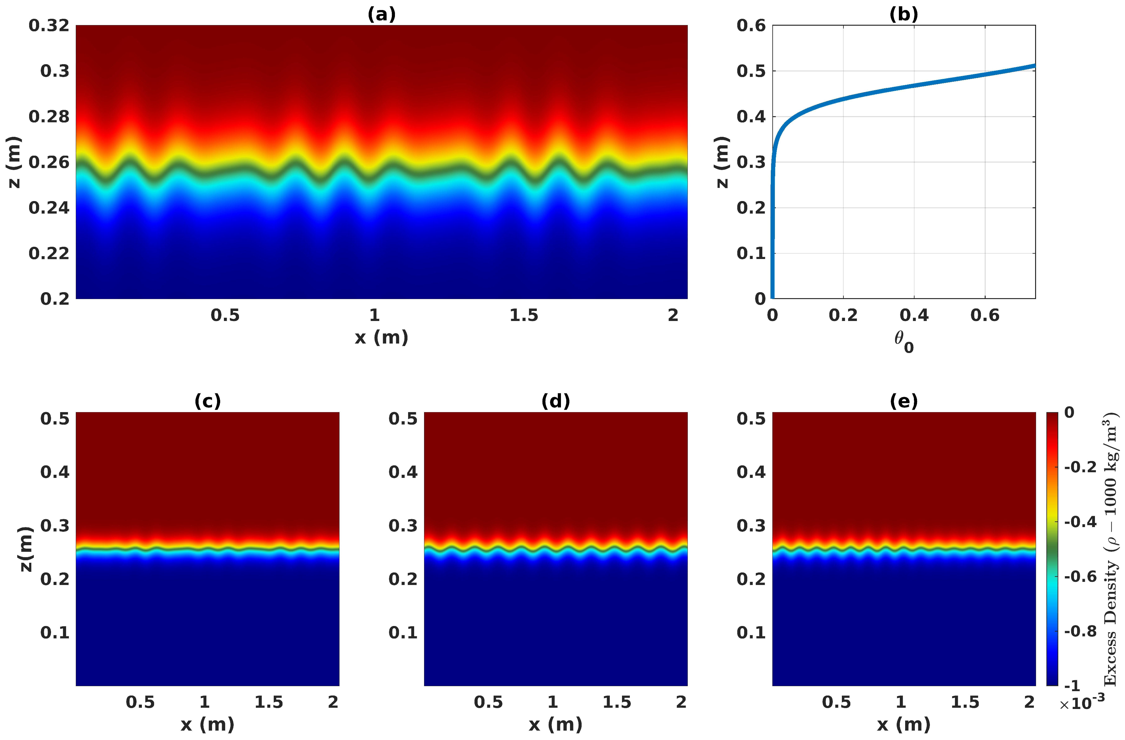
2.2. Numerical Simulation Ensemble Setup

We used the pseudospectral model SPINS to carry out direct numerical simulations of the Rayleigh–Taylor instability. The model uses third-order-accurate, variable time step Adams–Bashforth time-stepping and has spectral accuracy in space. When compared to lower-order finite difference or volume schemes with the same resolution, the numerical errors are much smaller [54]. Further, the numerical dispersion and diffusion errors often found in classical lower-order methods are absent from spectral methods. The SPINS code has been extensively validated against linear theory (e.g., growth rate for shear instability and internal wave generation [52]), existing numerical methods (e.g., in the context of dipole–wall collisions [52]), exact solutions (e.g., for the propagation of exact internal solitary waves [55]), and experimental data (e.g., cross-boundary layer transport due to shoaling mode with two internal waves [56]).

The simulation parameters and dimensionless numbers are given in

Table 1. Simulation parameters and dimensionless numbers.

Simulation Parameter	Value	Dimensionless Number	Value
$L_x$	2.048 m	$Re$	$1.1264\times {10}^4$
$L_z$	0.512 m	$Sc$	$7.1429$
$N_x$	4096	$Pe$	$8.0457\times {10}^4$
$N_z$	1024	$Da$	$2.3273$
g	9.81 m/s${}^2$
${\rho }_0$	1000 kg/m${}^3$
$\nu$	$1\times {10}^{-6}$ m${}^2$/s
$\kappa$	$1.4\times {10}^{-7}$ m${}^2$/s

. All simulations were run in two dimensions with a 2.048 m wide and 0.512 m tall domain. We used 4096 grid points in the horizontal and 1024 in the vertical to have a 0.5 mm resolution in both directions. Periodic boundary conditions were implemented in x and free slip boundary conditions were implemented in z.

All simulations begin from a state with $\overrightarrow{u}=0$. To induce the formation of Rayleigh–Taylor (RT) instabilities, each ensemble member is initialized with an unstable density stratification that is perturbed in the horizontal. The density and velocity fields thus take the forms

$$\begin{array}{}\mathrm{(15)}& \hfill \rho (\overrightarrow{x},t=0)& =-5\times {10}^{-4}\left(1-tanh\left(\frac{z-0.256-\epsilon \left(x\right)}{0.02}\right)\right),\hfill \mathrm{(16)}& \hfill \epsilon \left(x\right)& =2.5\times {10}^{-3}\sum _{i=1}^4{Y}_{1i}sin\left(\frac{16\pi (Y_{2i}+1)}{2.048}x+2\pi Y_{3i}\right),\hfill \mathrm{(17)}& \hfill \overrightarrow{u}(\overrightarrow{x},t=0)& =0,\hfill \end{array}$$

where $Y_{ji}\sim U(0,1)$ is a random variable chosen from a uniform distribution between 0 and 1. Following standard practice, the random number generator for the distribution is seeded by the fastest-changing portion of the clock-time at the start of each simulation. The only difference between ensemble members is the perturbation, $\epsilon$, applied to the initial density stratification. The initially unstable density stratification leads to the formation of RT instabilities. By perturbing the density interface in each simulation, we create lateral variability between ensemble members as the large-scale dynamics of RT instabilities maintain some memory of the initial conditions of the system [50].

The instability growth is exponential in time and a quasi-turbulent state is reached by $t=26$ s. We generate an ensemble of 50 simulations (i.e., 50 realizations of the quasi-turbulent state), storing the initial condition of each and then storing data every two seconds from $t=14$ s to $t=40$ s. This yields 2.5 G of data per ensemble member and a total of 125 G of data for subsequent analysis of the ensemble. Each of these relatively small simulations takes roughly 4 h to run with 16 cores, giving a total of 200 h of computing time.

Panel (a) of Figure 1 shows an example stratification from a subdomain of one of the simulations. In panels (c) through (e), the initial stratification in three other ensemble members are shown. The distinction between ensemble members comes from the perturbations, $\epsilon$, to the density stratification which are observable by comparing the panels.

Estimates of the dimensionless numbers were calculated using the domain height as the characteristic length scale and the maximum root-mean-square vertical velocity of a sample ensemble member as the velocity scale. The values are given in Table 1. The Reynolds number, $Re=UL/\nu$, represents the ratio of the inertial to viscous forces. Our simulations have $Re\approx 1.1264\times {10}^4$, indicating the flow becomes turbulent. The Schmidt number, $Sc=\nu /\kappa =7.1429$, tells us the momentum diffusivity is greater than that of the tracers. The Péclet number describes the ratio of advective to diffusive transport and is given by $Pe=Sc·Re\approx 8.0457\times {10}^4$.

In each of the simulations, the reaction term is

$$\begin{array}{c}\hfill F\left(\theta \right)=0.1·\theta (1-\theta )·tanh(\theta /0.001),\end{array}$$

(18)

where the multiplication by the hyperbolic tangent ensures that any oscillations around the unstable equilibrium $\theta =0$ are suppressed. The reaction timescale parameter $\alpha =0.1$ was chosen so that the Damköhler number, which we define as $Da=\frac{\alpha L}{U}\approx 2.3273$, was $O\left(1\right)$. The order of $Da$ was chosen to balance the reaction and advective timescales for the purpose of illustration. A fast reaction (e.g., $\alpha =1$) has $\theta \to 1$ too quickly for structures created by turbulent mixing to be observed. Slow reactions (e.g., $\alpha =0.01$) allow for the creation of sharp fronts, which can be difficult to resolve.

The initial distributions of both the reactive and passive tracers are given by

$$\begin{array}{cc}\hfill \theta (\overrightarrow{x},t=0)& \hfill =0.5\left(1+tanh\left(\frac{z-0.48}{0.06}\right)\right),\hfill \end{array}$$

(19)

so that the tracers lie in a band along the top of the domain, as shown in panel (b) of Figure 1. Each simulation evolves both tracers with the same velocity fields and the tracers do not interact. The simulations are stopped after 40 s, by which time the system has reached a well-mixed state.

3. Results

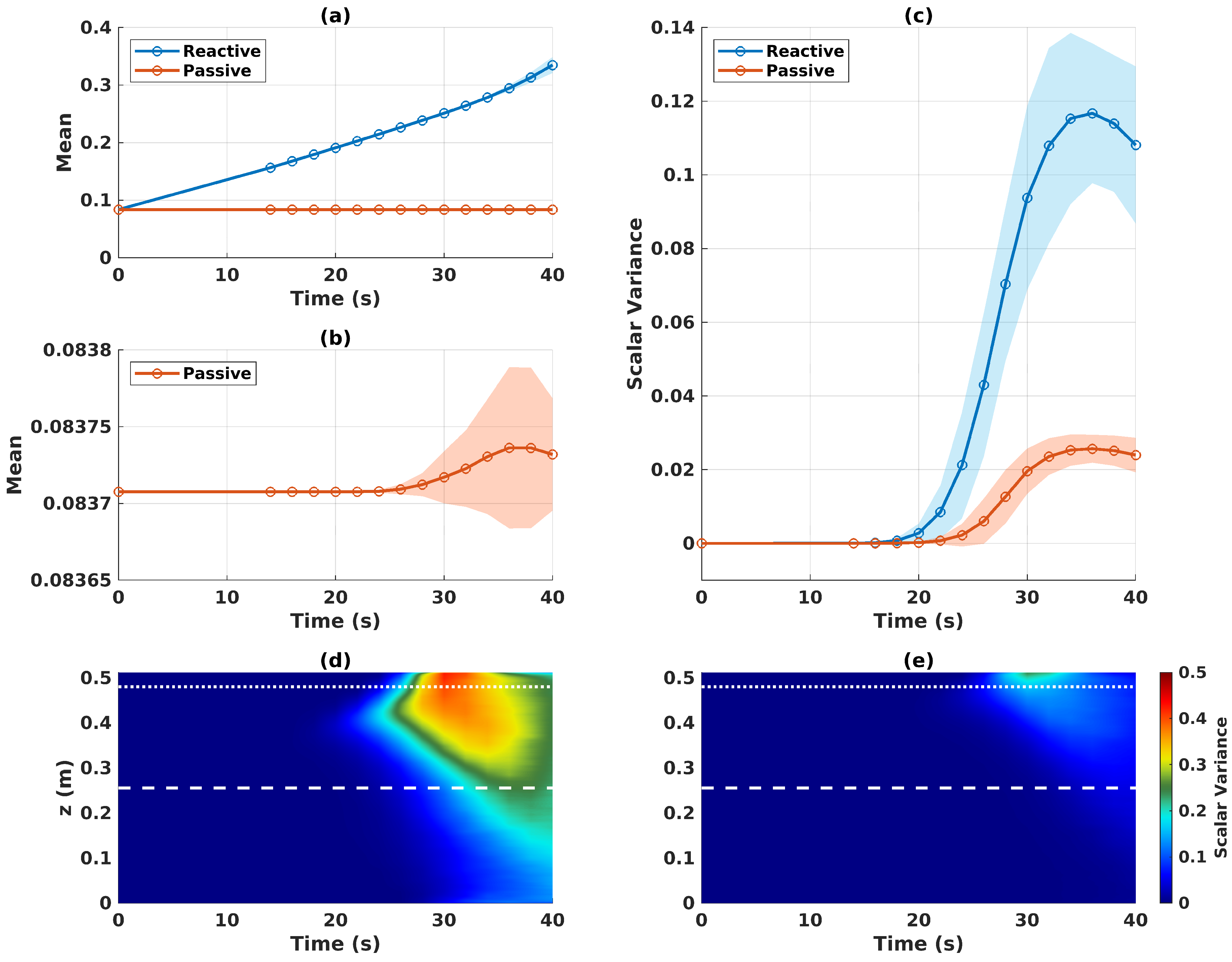
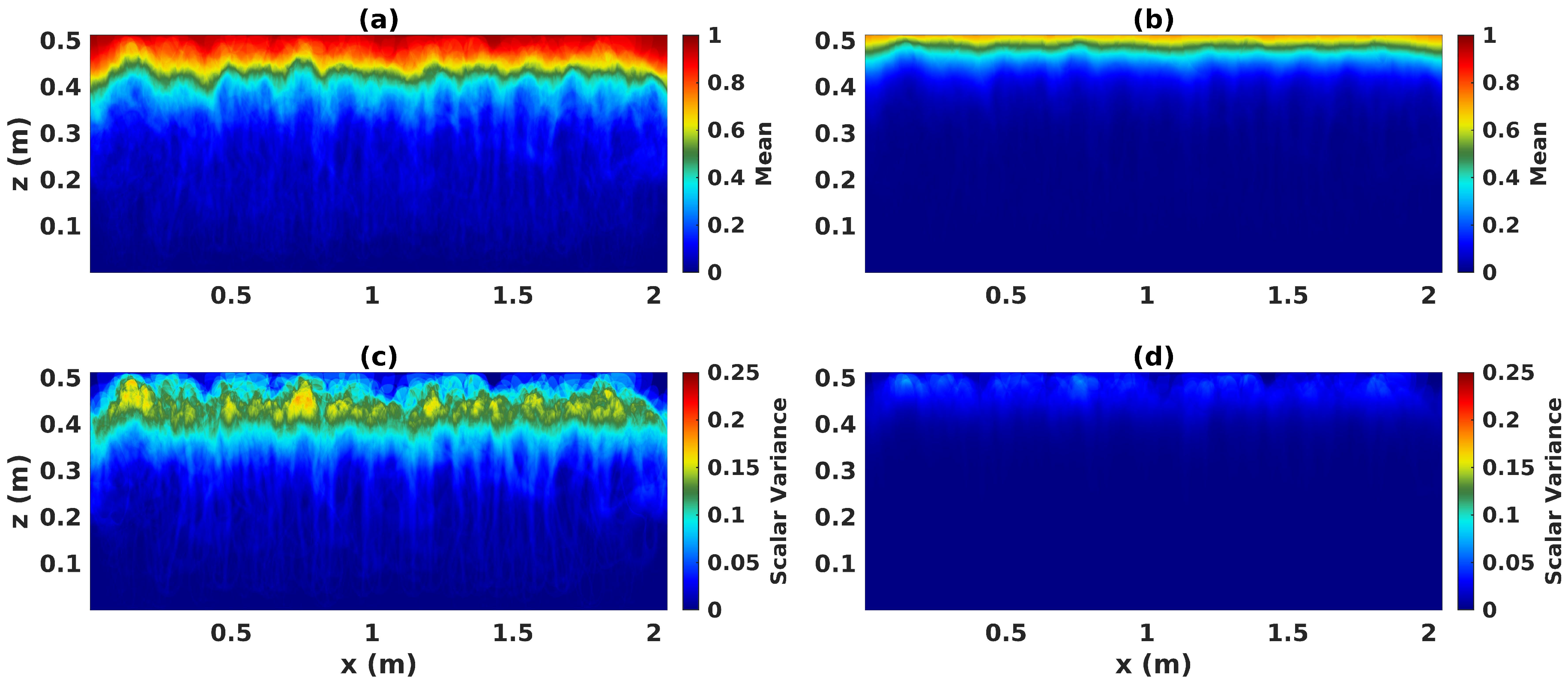
3.1. Tracer Mean and Scalar Variance

The reactive and passive tracers start in a band along the top of the domain with their concentrations decreasing downwards. Initially, the system is at rest to mimic the accumulation of a tracer in calm waters. If the system started out as turbulent, we would expect the tracer to be well-mixed, and since turbulent mixing is inherently unpredictable, it would be challenging to draw clear comparisons between the spatial distributions of the reactive and passive tracers. The initial density stratification is centered at $z=0.256$ m, about 0.16 m below the bottom of the tracer band. There is, thus, a delay between the start of the simulation and the time at which the RT instabilities start advecting the tracers. During this time, the tracers begin diffusing downwards and the reactive tracer grows according to the function in Equation (18). The reaction both increases the concentration of the tracer and accelerates the downwards spread by enhancing Fickian diffusion. Therefore, the reactive tracer front extends lower into the domain, allowing the RT plumes to reach it sooner than the passive tracer front.

Figure 2 (stills taken from Supplementary Movies S1 and S2) shows the (a) mean and (b) scalar variance of the reactive tracer at $t=26$ s. When comparing these quantities with those of the passive tracer, panels (b) and (d), it is clear that the the reactive tracer ensemble mean has a magnitude nearly twice that of the passive tracer and extends further downwards. In panels (a) and (b) of Figure 3, the bulk values of the means of the reactive (blue) and passive (orange) tracers are plotted as functions of time. The mean reactive tracer concentration nearly quadruples, while changes in the mean passive tracer concentration are $O\left({10}^{-5}\right)$ and likely due to the filter used in the numerical method. Note that in all of the figures presented herein, the shaded areas extend two standard deviations away from the corresponding ensemble means.

The ensemble is designed for the RT plumes in each simulation to have different spatial distributions. In each simulation, the RT bubbles (plumes of light fluid rising into heavy fluid with mushroom-shaped heads) push up against the tracer front and the tracer concentration is displaced upwards and outwards around the bubble. Meanwhile, spikes entrain the tracers downwards, causing the streaks observed in Figure 2. Shear causes vorticial structures to form on the undersides of the mushroom-shaped plume heads. These vortices are the first manifestation of turbulence in the flow and begin mixing the tracer that is displaced around the RT bubbles.

However, this behavior is not obvious in the Supplementary Movies showing the evolution of the mean and scalar variance fields for each of the tracers. When taking the mean of an ensemble, the structures present in the flows of the individual simulations are averaged out. So, the mean tracer fields do not show any of the coherent structures that characterize turbulent mixing. Instead, the structures are captured by the fluctuations, defined as differences between the individual simulations and the ensemble mean. The tracer fields in each of the simulations begin to differ from the mean as soon as the RT plumes start affecting their spatial distribution. Panel (c) of Figure 3 indicates a sharp increase in the scalar variance of the reactive tracer (blue) at $t=18$ s, as the RT bubbles reach the tracer front. It takes longer for the plumes to reach the passive tracer front.

The turbulence in each of the simulations deforms and contorts the material volumes of the conserved scalar, in this case our passive tracer, and increases the magnitude of local scalar gradients. This, in turn, enhances molecular diffusion [22]. When this same process acts on the reactive tracer, the reaction occurring within the material volume complicates things further. For growth governed by Fisher’s equation, the concentration in each material volume increases towards the stable equilibrium value $\theta =1$, thereby increasing the rate of molecular diffusion. This doubly enhanced diffusion allows the reactive tracer to spread to areas a passive tracer may not be able to reach. As the process of deformation by the flow is repeated, diffusion is further enhanced.

The scalar variance of the reactive tracer acts as a sink in the mean ADR equation (Equation (13)) and as a source in the fluctuation equation (Equation (14)). The fluctuations are effectively taking concentration from the mean field while also growing according to Fisher’s equation. In panels (a) and (c) of Figure 2, the spatial distribution of the scalar variance matches the front of the mean field. Looking at Supplementary Movie S1, we see that as the mean extends downwards, its concentration is transferred to the scalar variance, which evolves into a band spanning the domain horizontally. Eventually, the system becomes so well-mixed that the differences between simulations become less noticeable and thus the scalar variance decreases; Figure 3, panel (c).

By comparing the evolution of the reactive tracer with that of the passive tracer, we see that in the latter case the RT instabilities quickly break the mean structure apart, thereby increasing the scalar variance. However, the magnitude of the scalar variance is limited by the initial concentration of the tracer. In panels (d) and (e) of Figure 3, the reactive and passive scalar variances are integrated with respect to x and plotted as a function of depth and time. The dotted white lines indicate the inflection point of the hyperbolic tangent function describing the initial tracer distribution and the dashed line indicates the height of the mean initial density stratification. It is apparent that the scalar variance corresponding to the reactive tracer begins to increase lower in the domain as the tracer front has extended further downwards. We also notice that the scalar variance propagates both upwards and downwards. The upwards propagation corresponds to the transfer of concentration from the mean to the fluctuations while the downwards propagation is uniquely due to RT-induced turbulent mixing. The scalar variance of the passive tracer can only propagate downwards and is significantly smaller in magnitude.

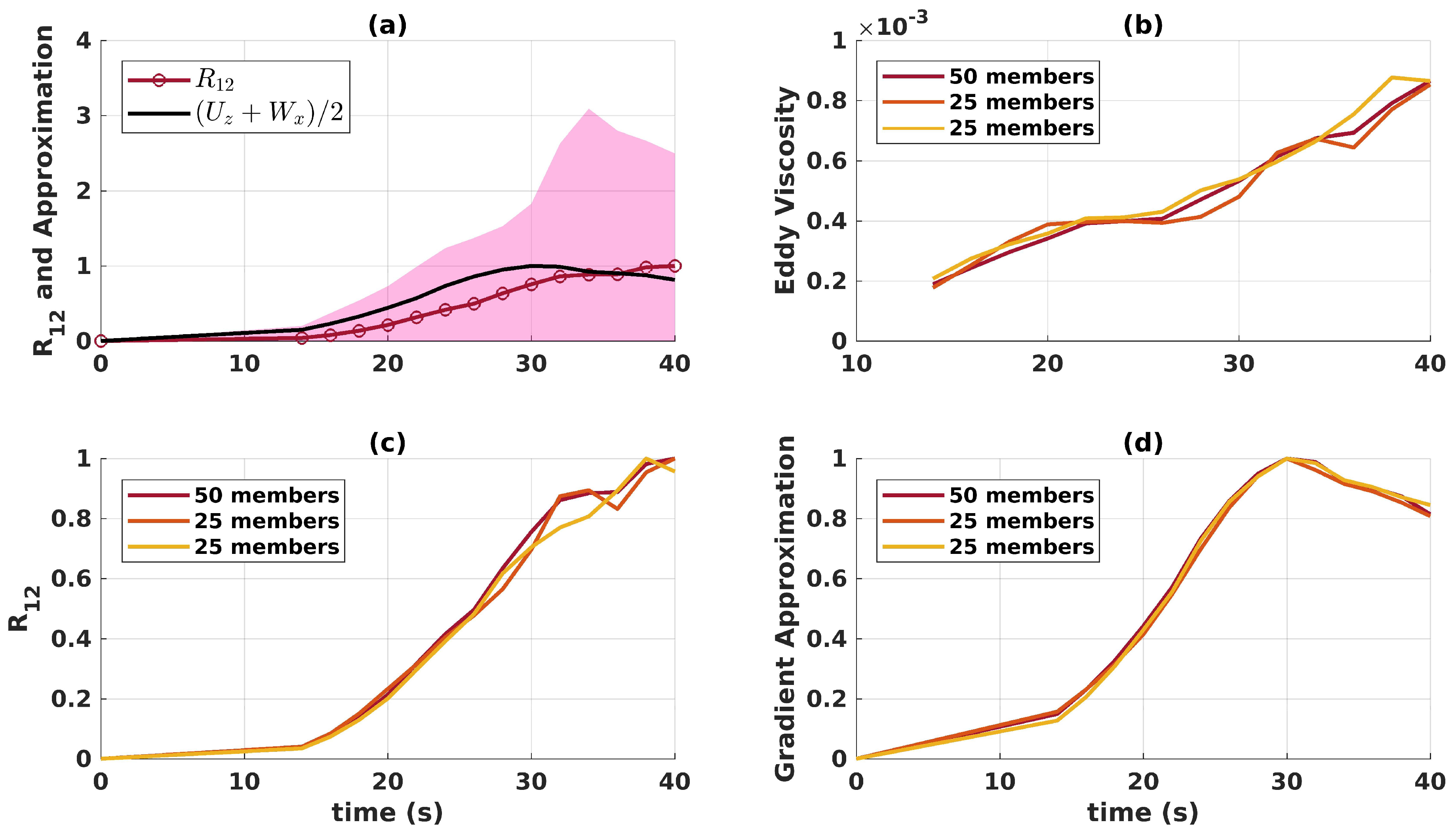
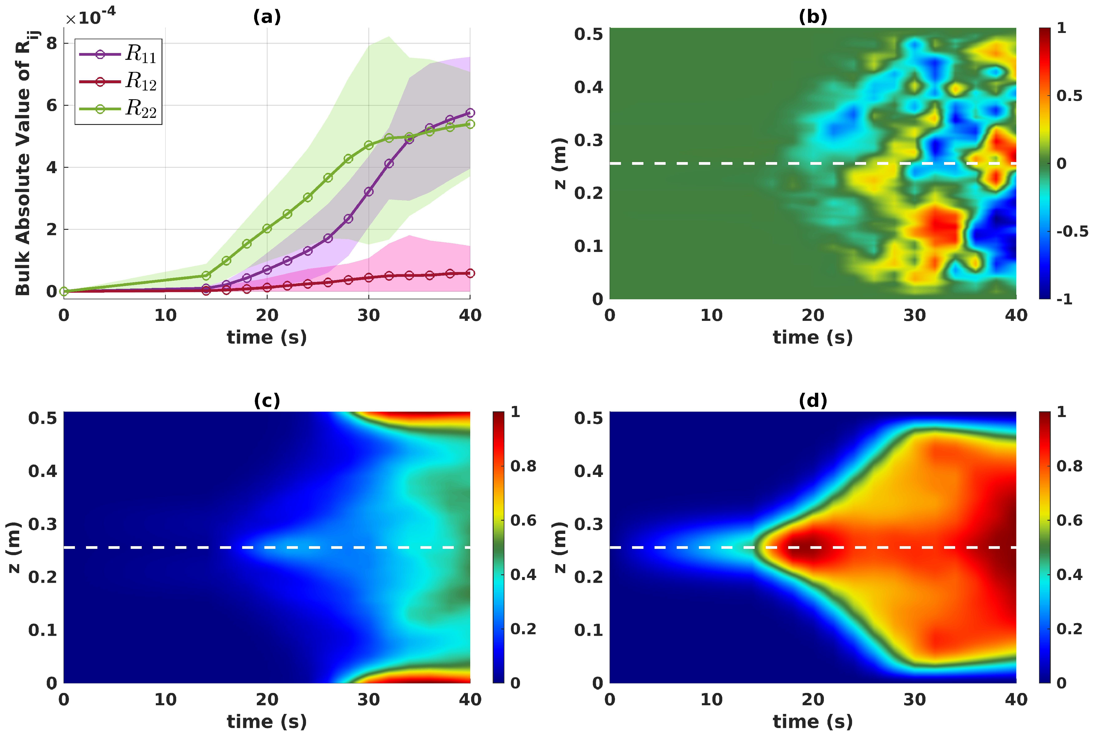
3.2. Reynolds Stresses

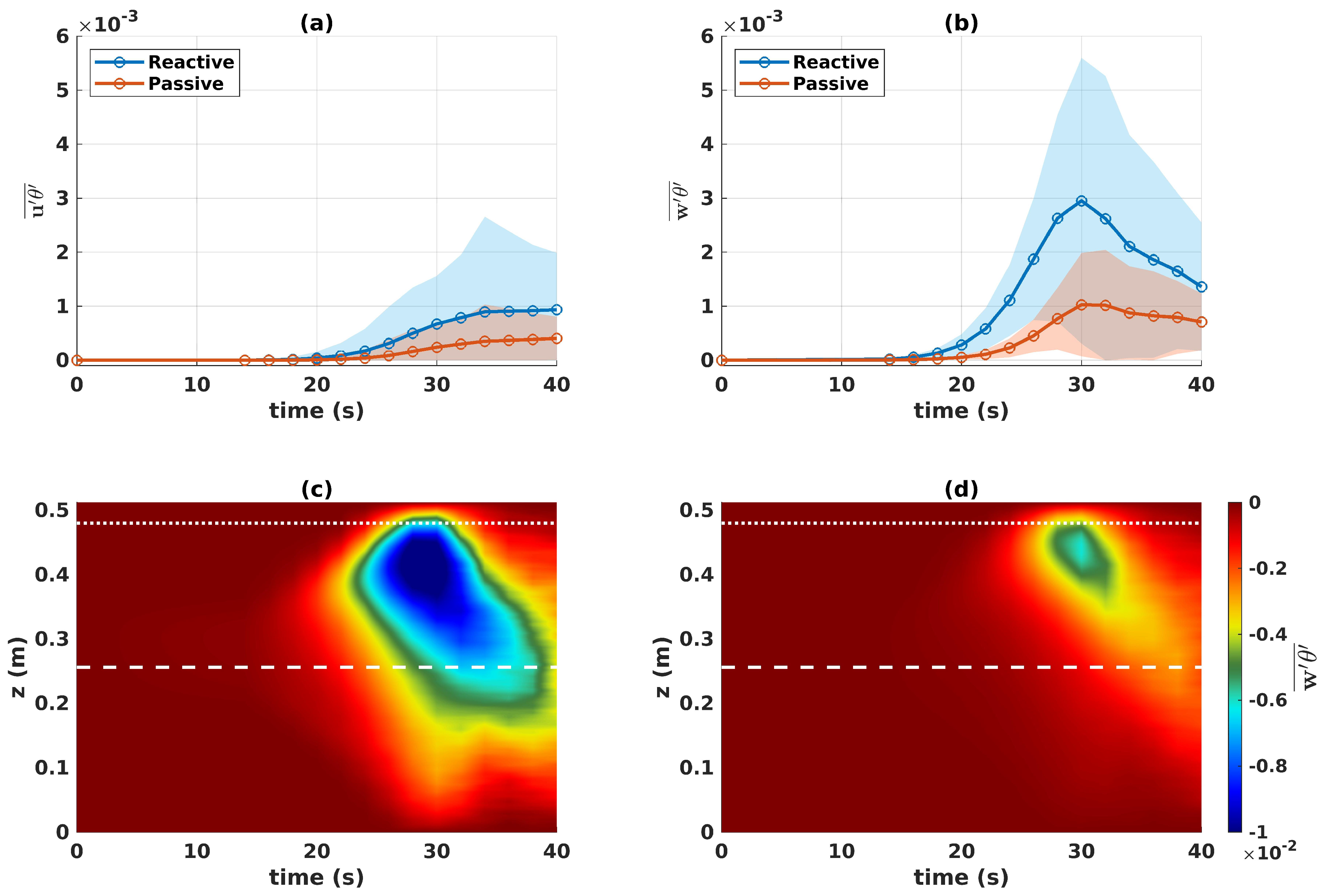
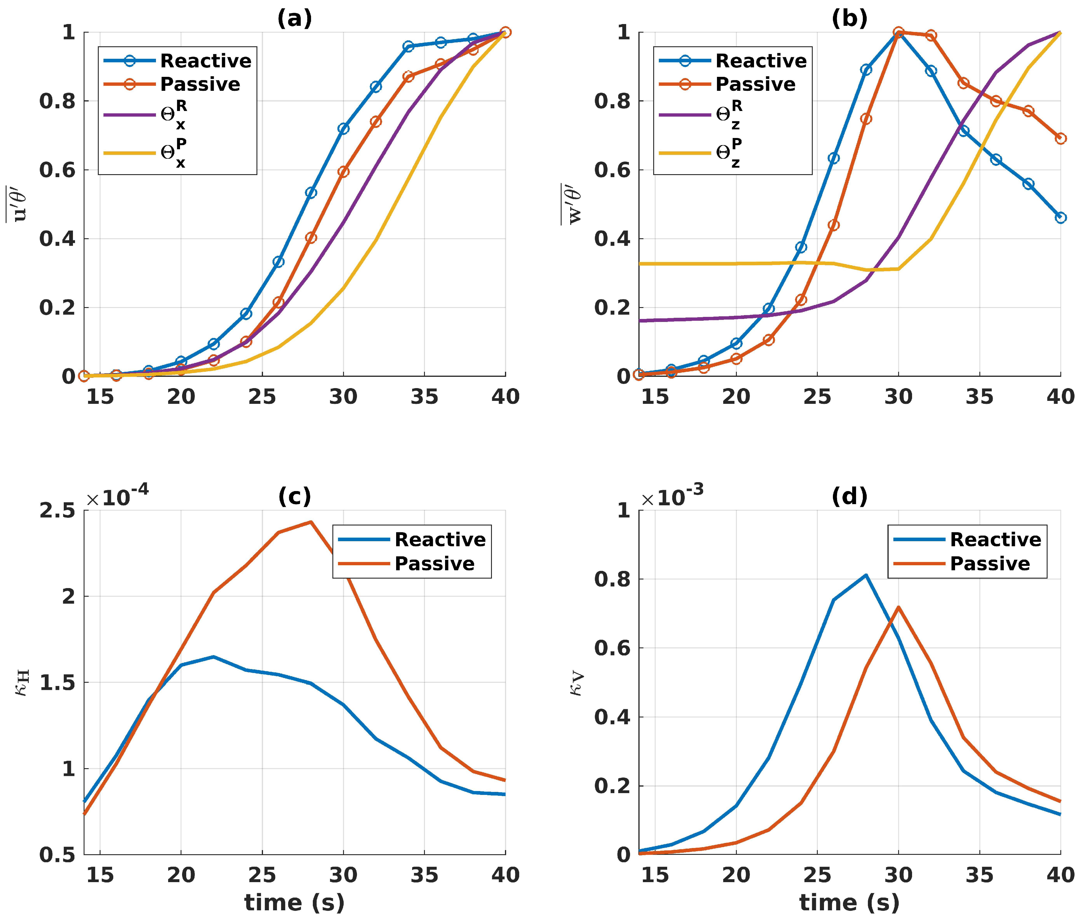
The bulk absolute values of the Reynolds stresses are depicted as functions of time in panel (a) of Figure 4. The shear stress is much weaker than the other stresses (though still on the same order of magnitude) and we note $R_{22}$ varies the most between ensemble members. Panels (b) through (d) show the normalized Reynolds stresses integrated with respect to x as a function of z and time. The dashed white lines indicate the initial height of the mean density stratification. From panel (d), we see that $R_{22}$ spreads symmetrically from the location of the initial stratification, which is in agreement with RT theory. The spatial distribution of $R_{11}$, panel (b), indicates that fluctuations in the horizontal velocity are symmetrical in z, greatest along the sidewalls, and take longer to increase than those in the vertical. The distribution of the shear stress is very different from those of $R_{11}$ and $R_{22}$. There is no symmetry around the initial stratification, nor is there a coherent pattern.

When using an eddy viscosity parameterization, we have [15]

$$\begin{array}{c}\hfill -R_{ij}={\nu }_e{\overline{S}}_{ij}-k{\delta }_{ij}\end{array}$$

(20)

where the mean rate of strain is given by

$$\begin{array}{c}\hfill {\overline{S}}_{ij}=\frac{1}{2}\left(\frac{\partial U_i}{\partial x_j}+\frac{\partial U_j}{\partial x_i}\right),\end{array}$$

(21)

and the turbulent kinetic energy (TKE) is defined as

$$\begin{array}{c}\hfill k=\frac{1}{2}(\overline{u^{\prime }{u}^{\prime }}+\overline{w^{\prime }{w}^{\prime }}).\end{array}$$

(22)

The Kronecker delta is denoted by ${\delta }_{ij}$, and ${\nu }_e$ is a phenomenological constant that needs to be selected as the “best” representation of the turbulence. Like the components of $R_{ij}$, k would be an unknown quantity in a RANS simulation. We have an ensemble of DNS simulations, so we have access to both the averaged and fluctuating quantities. Since we are interested in the downward propagation of the tracer front due to the downward transport of horizontal momentum, we focus on the $R_{12}$ component in what follows.

The spatial distribution of $R_{12}$ can be obtained from our data, so we can diagnose a time-dependent eddy viscosity defined as

$$\begin{array}{c}\hfill {\nu }_e=\frac{{\overline{S}}_{12}}{R_{12}}\end{array}$$

(23)

In panel (a) of Figure 5, the absolute value of the off-diagonal component of the Reynolds stress tensor is integrated in space and normalized. The shaded area extends two standard deviations (calculated using $u^{\prime }{w}^{\prime }$ from each ensemble member) away from the Reynolds stress and is also scaled by $max\left(\right|R_{12}\left|\right)$. The black line indicates the normalized eddy-viscosity approximation given by the right-hand side of Equation (20). The trend in $R_{12}$ is not well represented by the corresponding entry in the mean rate-of-strain tensor, ${\overline{S}}_{12}$. While $R_{12}$ increases monotonically, the eddy-viscosity approximation reaches its maximum at $t=30$ s and then begins to decrease. The calculations were performed with the entire ensemble as well as two unique subsets of 25 members each. In panels (c) and (d), we see that the normalized quantities collapse to nearly the same curve no matter the number or set of ensemble members considered. Panel (b) of Figure 5 shows the time-dependent eddy viscosity obtained according to Equation (23). Once again, the trend in the eddy viscosity is largely unaffected by the ensemble members used for the calculation.

3.3. Eddy Fluxes

Eddy fluxes quantify the mean transport of tracer fluctuations by fluctuations in the velocity fields. In Section 3.2, the evolution of the fluctuations in the velocity fields was discussed. We saw that fluctuations in the vertical velocity component spread symmetrically from the location of the initial density stratification while fluctuations in the horizontal one are largely found along the top and bottom boundaries. In Figure 6, we compare the bulk absolute horizontal and vertical eddy fluxes in panels (a) and (b) for the reactive (blue) and passive (orange) tracers. In Section 3.1, we saw that reactive tracer fluctuations are larger than those of the passive tracer. It thus comes as no surprise that the eddy fluxes corresponding to the reactive tracer are larger than those of the passive tracer.

Despite the magnitudes of the horizontal, $R^{11}$, and vertical, $R^{22}$, Reynolds stresses being similar, it is clear that the tracer fluctuations are more closely correlated with the vertical velocity fluctuations than the horizontal ones. Around $t=30$ s, the heads of the RT plumes collide with the top and bottom boundaries of the domain. At this time, the vertical eddy fluxes reach their maxima and subsequently decrease because the tracers cannot be advected any further in the vertical. The decrease in the vertical eddy flux of the reactive tracer is more dramatic than that corresponding to the passive tracer since fluctuations in the passive tracer barely reach the bottom of the domain and, thus, are not significantly affected by the bottom boundary.

In panels (c) and (d) of Figure 6, the vertical eddy fluxes of the reactive and passive tracers are integrated with respect to x and shown as functions of depth and time. The dotted white lines indicate the inflection point of the hyperbolic tangent function describing the initial tracer distribution and the dashed lines indicate the initial height of the mean density stratification. For both tracers, the vertical eddy fluxes are negative because, as shown in the Supplementary Movies, the fluctuations are traveling downwards. The heights at which the eddy fluxes first become nonzero align with the locations of the tracer fronts. The reactive tracer fluctuations and fluctuations in the vertical velocity field both propagate upwards (Figure 3 and Figure 4) making the vertical eddy flux propagate upwards. This does not necessarily imply that the fluctuations are being transported upwards. Rather, it tells us that the fluctuations develop higher in the domain as concentration is pulled from the ensemble mean. This is particularly evident in the Supplementary Movie of the reactive tracer fields (S1). These space–time plots further support the conclusion that the decrease seen in the bulk absolute vertical eddy flux of the reactive tracer is more dramatic because fluctuations in the passive tracer barely reach the bottom of the domain.

When running RANS simulations, eddy diffusivity parameterizations of the form

$$\begin{array}{c}\hfill -\overline{u^{\prime }{\theta }^{\prime }}={\kappa }_H\frac{\partial \theta }{\partial x},-\overline{w^{\prime }{\theta }^{\prime }}={\kappa }_V\frac{\partial \theta }{\partial z},\end{array}$$

(24)

are often used in place of the eddy fluxes, which are unknown. In Section 3.2, we saw that the eddy viscosity parameterization does not capture the same trends as the off-diagonal Reynolds stresses if the eddy viscosity is assumed to be constant. This does not inspire much confidence in the performance of the analogous eddy diffusivity parameterization. In panels (a) and (b) of Figure 7, the normalized bulk absolute eddy fluxes are plotted along with the normalized right-hand sides of the equations in (24). The tracer derivatives taken with respect to x capture the general behavior of the horizontal eddy fluxes but fail to capture the details. The horizontal eddy fluxes start increasing earlier and begin to plateau at late times.

The tracer derivatives taken with respect to z fail to capture even the general behavior of the vertical eddy fluxes. In particular, they do not capture the peak and subsequent decrease shown in the blue and orange curves of panel (b) in Figure 7. Rather, they increase almost monotonically (the exception being in the z derivative of the mean passive tracer around $t=30$ s). Due to the initial tracer stratifications, the derivatives with respect to z are initially nonzero. Since the simulations are initialized with $\overrightarrow{u}=0$, fluctuations in the velocity field only begin to appear as the Rayleigh–Taylor instability develops. Therefore, there is a clear mismatch between the vertical eddy fluxes and their eddy diffusivity parameterizations.

As previously discussed, the vertical eddy fluxes peak when tracer fluctuations reach the bottom of the domain. Eddy diffusivity parameterizations consider the gradient of the tracer mean, which only begins to reach the bottom boundary when the simulations are stopped and the tracer is well-mixed. In panels (c) and (d), we plot the corresponding vertical and horizontal eddy diffusivities obtained from dividing through by the tracer derivatives. The horizontal eddy diffusivities are an order of magnitude smaller than the vertical ones. The variability in the values brings the use of constant eddy diffusivities into question.

Bulk descriptions do not capture any information about the directions of the eddy fluxes or gradients. The angle between the vectors $({\Theta }_x,{\Theta }_z)$ and $(-\overline{u^{\prime }{\theta }^{\prime }},-\overline{w^{\prime }{\theta }^{\prime }})$ can be calculated at each grid point and indicates whether the eddy diffusivity parameterization is diffusing the tracer in the correct direction. Figure 8 presents the distribution of the grid points as a function of the absolute value of the angle between $({\Theta }_x,{\Theta }_z)$ and $(-\overline{u^{\prime }{\theta }^{\prime }},-\overline{w^{\prime }{\theta }^{\prime }})$. Note that the absolute angle is in $[0,\pi ]$ with a value of $\pi$ indicating that the vectors are anti-parallel. In this case, a negative eddy diffusivity would be required to realign them. The issue of negative diffusivities will be revisited in the discussion. The panels in Figure 8 show the distribution of angles at (a) $t=14$ s, as the RT instabilities are just forming; (b) $t=26$ s, when the RT plumes are large but have not reached the boundaries; and (c) $t=40$ s, when the system is well-mixed. In the early period, the distribution indicates that the eddy fluxes and gradient of the mean tracers are mostly aligned. The distribution then slumps towards $\pi$ and becomes fairly uniform by the end of the simulations. The eddy diffusivity parameterization performs better for the passive tracer than the reactive one, especially for intermediate times.

The spatial distribution of the angles in the upper portion of the domain is shown in Figure 9 at $t=26$ s for the (a) reactive and (b) passive tracers. At this time, Figure 2 shows that the mean front of the reactive tracer fluctuates around $z=0.4$ m and that of the passive tracer fluctuates around $z=0.48$ m (white lines in Figure 9). For the reactive tracer, the eddy fluxes and gradient are best aligned within the tracer band. For the passive tracer, the alignment is best in the area immediately underneath the front. Along the top boundary, the gradient and fluxes are generally perpendicular to one another. The mean tracer gradients do not take the effect of boundary conditions into account. The somewhat regular pattern in the distribution of the angle values along the top of the domain is the result of rising plume heads pushing fluid horizontally and downwards. Meanwhile, the tracer gradients are primarily pointing downwards, as the mean tracers lie in bands along the top of the domain. Therefore, the angles are primarily $\pm \pi /2$ in this region. So, while the eddy fluxes reflect properties of the flow governing the tracer transport, the gradients only reflect the spatial distribution of the mean tracer field.

The plumes formed by RT instabilities primarily move vertically, though the perturbations applied to the initial density stratification do encourage some plumes to propagate diagonally. If we consider the mean initial stratification, the perturbations average out. So, the mean effect of the RT instabilities is to transport the tracers vertically until turbulent mixing becomes strong enough to induce horizontal transport. At $t=26$ s, the mixing is strongest in the region where the eddy flux and gradient vectors are most aligned. In the passive tracer case, panel (b), we note that between $z=0.3$ m and $z=0.4$ m, the angle distribution is loosely arranged into columns. This is also true for the reactive tracer, panel (a), but less obvious because the reactive tracer fluctuations are larger and spread lower into the domain as the RT bubbles have already reached the tracer front, making the angle distribution more disordered. As previously mentioned, the increased Fickian diffusion exhibited by the reactive tracer will allow it to diffuse into turbulent structures and then be transported to regions that the passive tracer may not be able to reach. The reaction then causes this process to be repeated, enriching the fluctuation field.

4. Conclusions

Turbulent flows are highly unpredictable and disordered. In this study, small $O\left({10}^{-2}\right)$ perturbations to the shape of the initially unstable density stratification were enough to produce significant variability within an ensemble of 50 well-resolved simulations. RANS simulations implicitly assume that the most important dynamics are captured by the mean. We have shown that this assumption fails when considering the transport of a reactive tracer growing according to Fisher’s equation.

Under Reynolds averaging, the mean reaction equation is altered by the introduction of eddy reaction terms. The procedure in Section 2.1.2 can be applied to any polynomial reaction function. Even non-polynomial reaction functions could be subjected to the same procedure if they were approximated by Taylor polynomials. The procedure allows one to isolate the roles of the mean, fluctuations, and mean-fluctuation interactions in the Reynolds-averaged reaction function. It also tells us that any terms raised to an even power will introduce sources or sinks (depending on the sign of the coefficient) into the mean ADR equation which depend only on the fluctuations. For Fisher’s equation, a sink in the mean ADR equation transfers concentration from the mean to the fluctuations. Growth, whether in the mean or fluctuations, increases diffusion, allowing the reactive tracer to spread to parts of the domain that the passive tracer may not reach. These areas may include turbulent structures, further transferring concentration from the mean to the fluctuations. Diffusion and turbulent mixing push the tracer concentration away from its stable equilibrium, $\theta =1$, thereby promoting further growth and creating a positive feedback loop. Numerical dispersion, while not significant in our pseudospectral simulations, has the potential to artificially increase the diffusivity of a tracer. The positive feedback would, thus, be intensified in an inherently dissipative model (i.e., one based on finite volumes) such as ROMS [11].

Due to the flux of concentration from the mean to the fluctuations, the mean underestimates the tracer concentrations in the individual simulations. Further, as shown by the Supplementary Movies, the downwards propagation of the reactive tracer is captured by the fluctuations and not the mean. In a true RANS simulation, one has no knowledge of the Reynolds stresses, eddy fluxes, or eddy reactions. In our numerical experiment, these quantities have proven to have a significant effect on the downward propagation of the reactive tracer. The bulk scalar variances (which are also the eddy reactions for Fisher’s equation) for both the passive and reactive tracers are approximately one quarter of the magnitude of the corresponding bulk mean and, thus, certainly non-negligible.

Given the initial distribution of the tracers (panel (b) of Figure 1), the generation of turbulent mixing with an RT instability doomed the eddy diffusivity relations to fail. RT bubbles pushed up against the tracer fronts, causing counter-gradient fluxes and negative eddy diffusivities. As the fronts of the RT plumes hit the top and bottom of the domain, the flow transitioned from a state dominated by large-scale motions to one dominated by smaller-scale turbulent mixing. In the latter state, negative eddy diffusivities continue to be observed because the largest eddies are larger than the curvature of the mean vertical tracer profiles [18]. The reactive tracer fluctuations associated with the reaction–turbulence–diffusion feedback that was previously discussed can spread into large turbulent structures more easily than passive tracer fluctuations. Therefore, one would expect more counter-gradient flux associated with the reactive tracer, which is exactly what is observed in Figure 8. Negative eddy diffusivities have been observed in numerical studies of non-passive oceanic tracers and attributed to symmetric instabilities and other submesoscale phenomena [32], in agreement with the results presented herein. We would expect an eddy diffusivity parameterization to perform equally as badly if not worse for the same setup in three dimensions since the eddy diffusivity parameterization does not account for vortex tilting [22].

The simulations presented herein are two dimensional and thus cannot capture some aspects of oceanic flows. However, they do provide a simple turbulent $x-z$ flow and demonstrate that the coupling between turbulence and the reaction dynamics should not be ignored. This is an improvement over the toy flows that have been used to study the reaction dynamics of phytoplankton, for example, [37]. Rayleigh–Taylor flows were chosen because they result in primarily vertical transport and the downward propagation of the reactive tracer front. To keep the computational demand of running the ensemble reasonable, our simulations are two dimensional and performed in a relatively small domain. The domain size was chosen based on the requirement for 0.5 mm resolution to resolve the sharp reactive tracer fronts. Other flows may be more appropriate for representing convection in the oceanic boundary layer and this is an area for future work. The results presented herein consider how an ensemble average, or a Reynolds average, captures relevant dynamics. It is important to note that this quantity is not the same as that which would be obtained by running true RANS simulations.

5. Discussion

Due to the feedbacks observed between turbulent mixing and the reaction dynamics, we stress the importance of conducting studies of reactive tracers within turbulent flows. The use of convective cells to approximate turbulence is problematic primarily because the cells introduce streamlines that the tracer can only diffuse across [37,45]. In our study, turbulent RT-induced mixing created small, irregular structures that pulled the reactive tracer into parts of the domain it otherwise could not have reached. There was a significant amount of variability in the tracer distributions of our ensemble members. With pre-specified velocity fields, it will be near impossible to capture the structures that characterize turbulent mixing, and thus, variability in the tracer distribution will be underestimated.

In addition to the flow used to induce turbulent mixing, the results of this study are highly specific to the reaction and Damköhler number selected. We chose $Da\sim O\left(1\right)$ to balance the effects of advection with those of the reaction. The balance causes growth and mixing processes to become coupled and eddy diffusivity parameterizations to fail [36]. Ocean tracer dynamics are complex, so interactions between turbulent mixing and reaction dynamics are not as simple as the positive feedback we observed in our study [38,53,57].

When considering a slow reaction with $Da\sim O\left(0.1\right)$ or smaller, the coupling will be weaker, but new challenges arise as turbulent mixing creates sharp tracer filaments. Decreasing $Da$ to $O\left(0.1\right)$ made our 0.5 mm grid spacing insufficient to resolve the tracer filaments. This is problematic given the large disparity between the scale of our simulations and those of any regional modeling study. Increasing the diffusivity of the tracer would smooth out the fronts, thereby reducing the demand for a higher resolution. In a RANS simulation, this is achieved through eddy diffusivity parameterizations. Modeling studies based on ROMS generally have a $O\left(1\right)$ to $O\left(10\right)$-kilometer horizontal resolution and $O\left(1\right)$ to $O\left(100\right)$-meter vertical resolution [13,14,58]. Therefore, it should be assumed that tracer distributions in these models have been over-smoothed. Further, the spacing between ROMS grid points is not uniform and the vertical resolution is often better near the surface than at the bottom (O(1 m) versus O(200 m) [57]). A possible improvement may be simulating near surface effects, which are weighted more heavily due to the grid spacing, while parameterizing those deeper in the domain.

Thanks to our relatively small simulations, we were able to run an ensemble with 50 members. However, for larger, more complex simulations, the question of how many ensemble members to run is a tricky one to answer. In the limit of infinite ensemble members, we would expect quantities such as $\partial \Theta /\partial x$ and $\partial U/\partial z$ to vanish. In fact, when computing our results, we found that the mean tracer derivatives calculated with only half of the ensemble members demonstrated the same time-dependent trends, but had larger magnitudes. This was similar for $R_{12}$ and the derivatives of the mean velocities. Therefore, we present the results of Figure 5 and Figure 7 as normalized quantities and note that the eddy viscosity and diffusivities presented are functions of the ensemble members considered though their orders of magnitude remain unaffected. This brings into question how many ensemble members one should run when conducting studies of this form. The limiting behavior of an infinitely large ensemble varies drastically from the behavior observed in an individual simulation. Perhaps this is a reason to consider large eddy simulations over interpretations based on Reynolds averaging, and this is a planned avenue for future work.

Future directions for this work include running simulations with a deeper domain to allow for a longer transport period before the free slip walls begin to affect the flow. Though two-dimensional RT instabilities were sufficient for this study, their mixing characteristics are known to differ from their three-dimensional counterparts [47,50]. It would be interesting to determine whether a three-dimensional RT instability affects the reactive tracer any differently, for example, through organized larger-scale motions. Another possible avenue for exploration may be to use the data from the ensemble generated for this study to force simulations of the mean ADR equation. These simulations would allow the effects of the eddy flux and eddy reactions to be isolated and allow for the evaluation of potential parameterizations. Further, it would be worthwhile to investigate how the results presented herein relate to mesoscale eddy variability.

References

1. Triantafyllou, G.; Yao, F.; Petihakis, G.; Tsiaras, K.; Raitsos, D.; Hoteit, I. Exploring the Red Sea seasonal ecosystem functioning using a three-dimensional biophysical model. J. Geophys. Res. Ocean. 2014, 119, 1791–1811. [Google Scholar] [CrossRef]
2. Kamykowski, D. A preliminary biophysical model of the relationship between temperature and plant nutrients in the upper ocean. Deep Sea Res. Part A Oceanogr. Res. Pap. 1987, 34, 1067–1079. [Google Scholar] [CrossRef]
3. Resplandy, L.; Lévy, M.; McGillicuddy, D.J., Jr. Effects of eddy-driven subduction on ocean biological carbon pump. Glob. Biogeochem. Cycles 2019, 33, 1071–1084. [Google Scholar] [CrossRef]
4. Goldstein, E.D.; Pirtle, J.L.; Duffy-Anderson, J.T.; Stockhausen, W.T.; Zimmermann, M.; Wilson, M.T.; Mordy, C.W. Eddy retention and seafloor terrain facilitate cross-shelf transport and delivery of fish larvae to suitable nursery habitats. Limnol. Oceanogr. 2020, 65, 2800–2818. [Google Scholar] [CrossRef]
5. Baustian, M.M.; Meselhe, E.; Jung, H.; Sadid, K.; Duke-Sylvester, S.M.; Visser, J.M.; Allison, M.A.; Moss, L.C.; Ramatchandirane, C.; van Maren, D.S.; et al. Development of an Integrated Biophysical Model to represent morphological and ecological processes in a changing deltaic and coastal ecosystem. Environ. Model. Softw. 2018, 109, 402–419. [Google Scholar] [CrossRef]
6. Laurent, A.; Fennel, K.; Kuhn, A. An observation-based evaluation and ranking of historical Earth system model simulations in the northwest North Atlantic Ocean. Biogeosciences 2021, 18, 1803–1822. [Google Scholar] [CrossRef]
7. Haidvogel, D.B.; Arango, H.; Budgell, W.P.; Cornuelle, B.D.; Curchitser, E.; Di Lorenzo, E.; Fennel, K.; Geyer, W.R.; Hermann, A.J.; Lanerolle, L.; et al. Ocean forecasting in terrain-following coordinates: Formulation and skill assessment of the Regional Ocean Modeling System. J. Comput. Phys. 2008, 227, 3595–3624. [Google Scholar] [CrossRef]
8. Higdon, R.L.; Bennett, A.F. Stability analysis of operator splitting for large-scale ocean modeling. J. Comput. Phys. 1996, 123, 311–329. [Google Scholar] [CrossRef]
9. Shchepetkin, A.F.; McWilliams, J.C. The regional oceanic modeling system (ROMS): A split-explicit, free-surface, topography-following-coordinate oceanic model. Ocean Model. 2005, 9, 347–404. [Google Scholar] [CrossRef]
10. ROMS Wiki Vertical Mixing Parameterizations. Available online: https://www.myroms.org/wiki/Vertical_Mixing_Parameterizations (accessed on 18 August 2023).
11. Burchard, H.; Rennau, H. Comparative quantification of physically and numerically induced mixing in ocean models. Ocean Model. 2008, 20, 293–311. [Google Scholar] [CrossRef]
12. Brennan, C.E.; Bianucci, L.; Fennel, K. Sensitivity of northwest North Atlantic shelf circulation to surface and boundary forcing: A regional model assessment. Atmosphere-Ocean 2016, 54, 230–247. [Google Scholar] [CrossRef]
13. Kumar, R.; Li, J.; Hedstrom, K.; Babanin, A.V.; Holland, D.M.; Heil, P.; Tang, Y. Intercomparison of Arctic sea ice simulation in ROMS-CICE and ROMS-Budgell. Polar Sci. 2021, 29, 100716. [Google Scholar] [CrossRef]
14. Sui, Y.; Sheng, J.; Tang, D.; Xing, J. Study of storm-induced changes in circulation and temperature over the northern South China Sea during Typhoon Linfa. Cont. Shelf Res. 2022, 249, 104866. [Google Scholar] [CrossRef]
15. Pope, S.B. Turbulent Flows; Cambridge University Press: Cambridge, UK, 2000. [Google Scholar]
16. Dimotakis, P.E. Turbulent mixing. Annu. Rev. Fluid Mech. 2005, 37, 329–356. [Google Scholar] [CrossRef]
17. Sreenivasan, K.R. Turbulent mixing: A perspective. Proc. Natl. Acad. Sci. USA 2019, 116, 18175–18183. [Google Scholar] [CrossRef]
18. Kundu, P.K.; Cohen, I.M.; Dowling, D.R. Fluid Mechanics; Academic Press: Cambridge, MA, USA, 2015. [Google Scholar]
19. Alfonsi, G. Reynolds-averaged Navier–Stokes equations for turbulence modeling. Appl. Mech. Rev. 2009, 62, 040802. [Google Scholar] [CrossRef]
20. Xiao, H.; Cinnella, P. Quantification of model uncertainty in RANS simulations: A review. Prog. Aerosp. Sci. 2019, 108, 1–31. [Google Scholar] [CrossRef]
21. Pozorski, J.; Minier, J.P. Modeling scalar mixing process in turbulent flow. In Proceedings of the First Symposium on Turbulence and Shear Flow Phenomena, Santa Barbara, CA, USA, 12–15 September 1999; Begel House Inc.: Danbury, CT, USA, 1999. [Google Scholar]
22. Wyngaard, J.C. Turbulence in the Atmosphere; Cambridge University Press: Cambridge, UK, 2010. [Google Scholar]
23. Xiao, S.; Yang, D. Effect of oil plumes on upper-ocean radiative transfer—A numerical study. Ocean Model. 2020, 145, 101522. [Google Scholar] [CrossRef]
24. Abernathey, R.P.; Marshall, J. Global surface eddy diffusivities derived from satellite altimetry. J. Geophys. Res. Ocean. 2013, 118, 901–916. [Google Scholar] [CrossRef]
25. Cole, S.T.; Wortham, C.; Kunze, E.; Owens, W.B. Eddy stirring and horizontal diffusivity from Argo float observations: Geographic and depth variability. Geophys. Res. Lett. 2015, 42, 3989–3997. [Google Scholar] [CrossRef]
26. Marshall, J.; Shuckburgh, E.; Jones, H.; Hill, C. Estimates and implications of surface eddy diffusivity in the Southern Ocean derived from tracer transport. J. Phys. Oceanogr. 2006, 36, 1806–1821. [Google Scholar] [CrossRef]
27. Sallée, J.; Speer, K.; Morrow, R.; Lumpkin, R. An estimate of Lagrangian eddy statistics and diffusion in the mixed layer of the Southern Ocean. J. Mar. Res. 2008, 66, 441–463. [Google Scholar] [CrossRef]
28. Ferrari, R.; Nikurashin, M. Suppression of eddy diffusivity across jets in the Southern Ocean. J. Phys. Oceanogr. 2010, 40, 1501–1519. [Google Scholar] [CrossRef]
29. Holloway, G. Estimation of oceanic eddy transports from satellite altimetry. Nature 1986, 323, 243–244. [Google Scholar] [CrossRef]
30. Gargett, A.E. Vertical eddy diffusivity in the ocean interior. J. Mar. Res. 1984, 42, 359–393. [Google Scholar] [CrossRef]
31. Kamenkovich, I.; Berloff, P.; Haigh, M.; Sun, L.; Lu, Y. Complexity of mesoscale eddy diffusivity in the ocean. Geophys. Res. Lett. 2021, 48, e2020GL091719. [Google Scholar] [CrossRef]
32. Smith, K.M.; Hamlington, P.E.; Fox-Kemper, B. Effects of submesoscale turbulence on ocean tracers. J. Geophys. Res. Ocean. 2016, 121, 908–933. [Google Scholar] [CrossRef]
33. Radko, T. Double-Diffusive Convection; Cambridge University Press: Cambridge, UK, 2013. [Google Scholar]
34. Bachman, S.D.; Fox-Kemper, B.; Bryan, F.O. A tracer-based inversion method for diagnosing eddy-induced diffusivity and advection. Ocean Model. 2015, 86, 1–14. [Google Scholar] [CrossRef]
35. Pasquero, C. Differential eddy diffusion of biogeochemical tracers. Geophys. Res. Lett. 2005, 32. [Google Scholar] [CrossRef]
36. Prend, C.J.; Flierl, G.R.; Smith, K.M.; Kaminski, A.K. Parameterizing eddy transport of biogeochemical tracers. Geophys. Res. Lett. 2021, 48, e2021GL094405. [Google Scholar] [CrossRef]
37. Tergolina, V.B.; Calzavarini, E.; Mompean, G.; Berti, S. Effects of large-scale advection and small-scale turbulent diffusion on vertical phytoplankton dynamics. Phys. Rev. E 2021, 104, 065106. [Google Scholar] [CrossRef] [PubMed]
38. Richards, K.J.; Brentnall, S.J. The impact of diffusion and stirring on the dynamics of interacting populations. J. Theor. Biol. 2006, 238, 340–347. [Google Scholar] [CrossRef]
39. Lévy, M.; Martin, A.P. The influence of mesoscale and submesoscale heterogeneity on ocean biogeochemical reactions. Glob. Biogeochem. Cycles 2013, 27, 1139–1150. [Google Scholar] [CrossRef]
40. Zhang, J.; Tejada-Martínez, A.E.; Zhang, Q. Developments in computational fluid dynamics-based modeling for disinfection technologies over the last two decades: A review. Environ. Model. Softw. 2014, 58, 71–85. [Google Scholar] [CrossRef]
41. Zhang, J.; Tejada-Martínez, A.E.; Zhang, Q.; Lei, H. Evaluating hydraulic and disinfection efficiencies of a full-scale ozone contactor using a RANS-based modeling framework. Water Res. 2014, 52, 155–167. [Google Scholar] [CrossRef]
42. Angeloudis, A.; Stoesser, T.; Gualtieri, C.; Falconer, R. Effect of three-dimensional mixing conditions on water treatment reaction processes. In Proceedings of the 36th IAHR World Congress, Hague, The Netherlands, 28 June–3 July 2015. [Google Scholar]
43. Weerasuriya, A.U.; Zhang, X.; Tse, K.T.; Liu, C.H.; Kwok, K.C. RANS simulation of near-field dispersion of reactive air pollutants. Build. Environ. 2022, 207, 108553. [Google Scholar] [CrossRef]
44. Aubagnac-Karkar, D.; Michel, J.B.; Colin, O.; Vervisch-Kljakic, P.E.; Darabiha, N. Sectional soot model coupled to tabulated chemistry for Diesel RANS simulations. Combust. Flame 2015, 162, 3081–3099. [Google Scholar] [CrossRef]
45. Beltram Tergolina, V.; Calzavarini, E.; Mompean, G.; Berti, S. Surface light modulation by sea ice and phytoplankton survival in a convective flow model. Eur. Phys. J. Plus 2022, 137, 1387. [Google Scholar] [CrossRef]
46. Kelley, D.E. Convection in ice-covered lakes: Effects on algal suspension. J. Plankton Res. 1997, 19, 1859–1880. [Google Scholar] [CrossRef]
47. Cabot, W. Comparison of two-and three-dimensional simulations of miscible Rayleigh-Taylor instability. Phys. Fluids 2006, 18. [Google Scholar] [CrossRef]
48. Kokkinakis, I.W.; Drikakis, D.; Youngs, D.L. Modeling of Rayleigh-Taylor mixing using single-fluid models. Phys. Rev. E 2019, 99, 013104. [Google Scholar] [CrossRef]
49. Abarzhi, S.I. Review of theoretical modelling approaches of Rayleigh–Taylor instabilities and turbulent mixing. Philos. Trans. R. Soc. A Math. Phys. Eng. Sci. 2010, 368, 1809–1828. [Google Scholar] [CrossRef] [PubMed]
50. Dalziel, S.; Linden, P.; Youngs, D. Self-similarity and internal structure of turbulence induced by Rayleigh–Taylor instability. J. Fluid Mech. 1999, 399, 1–48. [Google Scholar] [CrossRef]
51. Zhou, Q. Temporal evolution and scaling of mixing in two-dimensional Rayleigh-Taylor turbulence. Phys. Fluids 2013, 25. [Google Scholar] [CrossRef]
52. Subich, C.J.; Lamb, K.G.; Stastna, M. Simulation of the Navier–Stokes equations in three dimensions with a spectral collocation method. Int. J. Numer. Methods Fluids 2013, 73, 103–129. [Google Scholar] [CrossRef]
53. Bracco, A.; Clayton, S.; Pasquero, C. Horizontal advection, diffusion, and plankton spectra at the sea surface. J. Geophys. Res. Ocean. 2009, 114. [Google Scholar] [CrossRef]
54. Trefethen, L.N. Spectral methods in MATLAB, volume 10 of Software, Environments, and Tools. Soc. Ind. Appl. Math. 2000, 24, 57. [Google Scholar]
55. Harnanan, S.; Soontiens, N.; Stastna, M. Internal wave boundary layer interaction: A novel instability over broad topography. Phys. Fluids 2015, 27. [Google Scholar] [CrossRef]
56. Deepwell, D.; Stastna, M.; Carr, M.; Davies, P.A. Interaction of a mode-2 internal solitary wave with narrow isolated topography. Phys. Fluids 2017, 29. [Google Scholar] [CrossRef]
57. Hopkins, J.E.; Palmer, M.R.; Poulton, A.J.; Hickman, A.E.; Sharples, J. Control of a phytoplankton bloom by wind-driven vertical mixing and light availability. Limnol. Oceanogr. 2021, 66, 1926–1949. [Google Scholar] [CrossRef]
58. Rutherford, K.; Fennel, K.; Atamanchuk, D.; Wallace, D.; Thomas, H. A modelling study of temporal and spatial pCO 2 variability on the biologically active and temperature-dominated Scotian Shelf. Biogeosciences 2021, 18, 6271–6286. [Google Scholar] [CrossRef]
Figure 1. (a,ce) Sample initial density stratifications perturbed by ε ( x ) (Equation (16)). (b) Initial tracer concentration profile.
Jmse 11 02036 g001
Figure 2. Mean and scalar variance of the reactive, (a,c) from Supplementary Movie S1, and passive, (b,d) from Supplementary Movie S2, tracers at t = 26 s.
Jmse 11 02036 g002
Figure 3. (a,b) Bulk mean tracer concentrations and (c) bulk scalar variances for the reactive (blue) and passive (orange) tracers. Shaded areas extend two standard deviations away from the mean. (d,e) Scalar variance integrated with respect to x for the reactive and passive tracers, respectively.
Jmse 11 02036 g003
Figure 4. (a) Bulk absolute Reynolds stresses, with shaded areas extending two standard deviations away from the mean. Normalized Reynolds stresses (b) R 12 , (c) R 11 , and (d) R 22 integrated with respect to x.
Jmse 11 02036 g004
Figure 5. (a) Normalized bulk mean Reynolds stress R 12 , with shaded areas extending two standard deviations away from the mean and corresponding normalized bulk gradient approximation ( U z + W z ) / 2 calculated with all 50 ensemble members. (b) Time-dependent eddy viscosities from Equation (20). (c) Normalized R 12 and (d) normalized gradient approximations for the entire ensemble and two unique subsets of 25 members.
Jmse 11 02036 g005
Figure 6. Bulk absolute value of the (a) horizontal and (b) vertical eddy fluxes of the reactive (blue) and passive (orange) tracers. Vertical eddy fluxes integrated with respect to x for the (c) reactive and (d) passive tracers.
Jmse 11 02036 g006
Figure 7. Normalized bulk absolute values of the (a) horizontal and (b) vertical eddy fluxes of the reactive (blue) and passive (orange) tracers. The bulk absolute values of the derivatives of the mean tracers are plotted for comparison. Time-dependent (c) horizontal and (d) vertical eddy diffusivities.
Jmse 11 02036 g007
Figure 8. Absolute angle between the eddy flux and gradient of the mean at (a) t = 14 s, (b) t = 26 s, and (c) t = 40 s quantified as a proportion of the total number of grid points.
Jmse 11 02036 g008
Figure 9. Angle between the eddy flux and gradient for the (a) reactive and (b) passive tracers at t = 26 s.
Jmse 11 02036 g009