Combined Coastal Sea Level Estimation Considering Astronomical Tide and Storm Surge Effects: Model Development and Its Application in Thermaikos Gulf, Greece

Abstract

Tide gauge recordings furnish the longest and almost the most continuous data source of sea level monitoring. Traditionally, they are collected using tide gauge instrumentation fixed at seaport locations to provide a time series of sea level estimates relative to a local geodetic benchmark. Sea level tidal observables are distinguished in the astronomical tide component originating from the attraction of the Earth–Moon–Sun gravitational system, and the storm surges ought to have meteorological effects due to wind and atmospheric air pressure variation. This study provides a comprehensive methodological approach and software to compute sea level considering astronomical tides enhanced by storm surge effects. The model is realized and assessed using a long-standing set of 21 consecutive years of tidal and meteorological measurements originating from Thermaikos Gulf, Greece. Analyses show model verification and conclusions about the tidal behavior of the test area, suggesting a satisfactory agreement (86% Willmott Skill factor, 9 cm standard deviation) between predicted and observed sea level estimates, accounting for amplitude and the time shift of skew surges.

1. Introduction

Sea level rise is an important consequence of the climate crisis because it induces a significant impact on human and natural systems. Scientific expeditions and studies ascertain a pattern of sea level rise at a global level [1], regional [2,3], and local scale [4] because of climate change. Potential consequences include flooding, coastal erosion, saltwater intrusion into low-lying aquifers, and the submergence of flat regions. Therefore, the monitoring and prediction of sea level change is a key element to sustainable planning of life in coastal regions [5,6,7,8,9,10]. However, in addition to contributing to climate change monitoring, sea level studies serve fundamental geosciences. Particularly, they provide the basis for the definition of height reference systems in geodesy [11,12,13], assist the investigation of vertical land motion [14,15], and overly, provide the infrastructure for maritime spatial planning [16].

Sea level variation is driven by a multitude of natural processes that vary both in spatial and temporal scale. In this regard, astronomical tide is a periodic phenomenon affecting sea level oscillation in a rather consistent way realized either on a day or half-day basis. Its amplitude depends primarily on geographic location featuring a temporal variation governed by the time of the day, the season of the year, and the Earth’s location in relation to the moon and the sun [17,18].

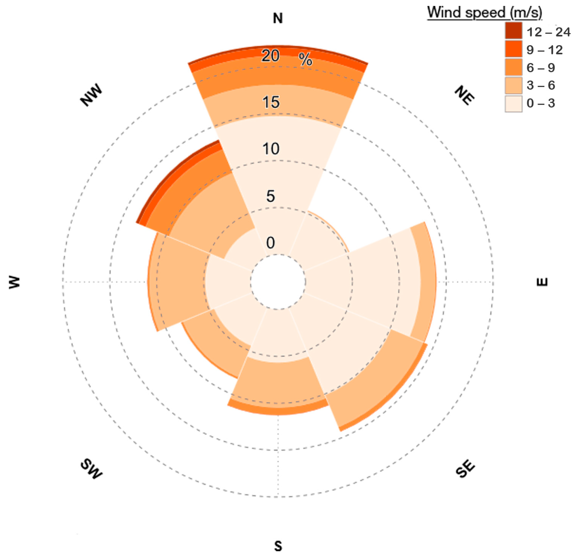
On the other hand, atmospheric force reflects the combined effect of air pressure and wind on sea level variation. Atmospheric effects usually last from hours to several days [19] before they gradually relent or migrate to another spot. Although meteorological tide (also known as storm surge) reflects the atmospheric contribution on sea level variation, it is sometimes treated or meant to be simply part of the sea level residuals that remain after subtracting the effect of the astronomical tide from sea level raw observables. However, according to the literature [17,20,21] and the analyses by the Intergovernmental Oceanographic Committee [22], the storm surge comprises an individual component of sea level variation rather than a residual value alone.

Sea level monitoring is usually realized locally using tide gauge recordings acquired at selected observation sites. Studies of sea level variation can also be undertaken on the open sea or the oceans using advanced propagation models relying on seashore information in conjunction with satellite altimetry. The monitoring and analysis of sea level variation have been studied extensively in the past; for instance, see [23,24,25,26,27,28,29,30]. These studies combine records from various sources including tide gauge stations, current meters, meteorological stations, and, in certain cases, satellite altimetry. However, historically, the backbone of sea level studies relies on data derived from tide gauges and meteorological stations of various types.

This paper provides a methodological approach for sea level estimation at a single site. Firstly, the astronomical effects that mainly govern sea level fluctuations are calculated, and secondly, tidal residuals are modeled considering the meteorological force effects. The proposed strategy takes into account an evaluation process comparing tide gauge data and the result of sea level modeling. The remaining residuals are partly ascribed to the presence and amplitude of skew surges. An analysis is undertaken in Thermaikos Gulf (north Greece) using historical tide gauge data obtained from the Thessaloniki harbor station spanning a period of 21 consecutive years. Meteorological data originate from the Thessaloniki National Airport weather station. Sea level information is distinguished by its astronomical and meteorological components [17]. Its variation is quantified through the amplitude and phase of tide constituents representing the astronomical tide on one hand and the atmospheric pressure and wind velocity for the storm surges on the other hand. Analyses yield conclusions about the tidal behavior of Thermaikos Gulf, indicating a suitable methodology for studying other areas of interest with similar characteristics.

This paper is structured as follows. Section 2 provides some insight into the theoretical background underlying this study and describes the study area and the available data in the tide gauge and the meteorological data located in Thermaikos Gulf. Section 3 presents, in detail, the implementation of the adopted modeling process and its associated evaluation procedure and metrics. Finally, Section 4 provides a discussion and conclusions on the main findings and perspectives of this study.

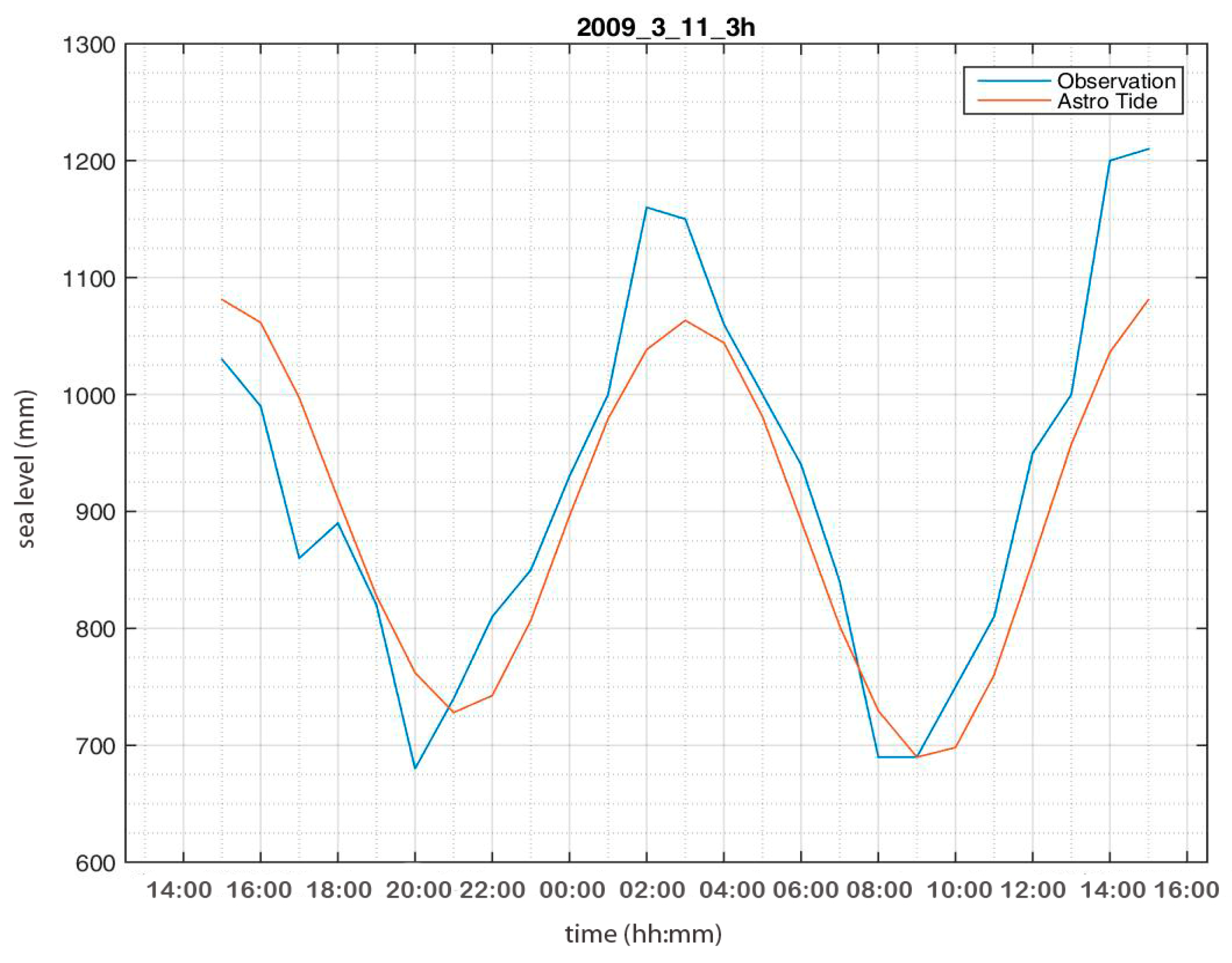
2. Materials and Methods

2.1. Tidal Components of Sea Level Estimation

Astronomical tide is the periodic movement of water level that is caused by the gravitational effect of the moon and the sun as they change their position in relation to the rotating Earth. In mathematics, the astronomical tide is realized through the summation of a number of distinct frequency cosine harmonics that exhibit an amplitude and a phase lag, the size of which depends on observation site location and time. Therefore, the amplitude of a tidal harmonic at a specific frequency (or speed) differs from place to place. Similarly, its phase component depends on the start time of a tidal signal analysis and site location. Furthermore, amplitude changes slightly with time following an 18.6-year circle [19]. To accommodate for this effect, a constant term is added, which represents a reference water level that is usually realized by the mean sea level. However, depending on specific data characteristics, mean sea level might also be a function of time [17].

Tidal constituents are derived by harmonic analysis of the sea level time series in accordance with Fourier transform. Spectral analysis forms the basis for studying any phenomenon of reparative nature [31,32,33]. Specifically, sea level composition or prediction is expressed as follows:

$$\mathrm{h}\left(\mathrm{t}\right)={\mathrm{h}}_0+{\sum }_{\mathrm{j}=1}^{\mathrm{m}}{\mathrm{R}}_{\mathrm{j}}\cos \left({\mathsf{\omega }}_{\mathrm{j}}\mathrm{t}-{\mathsf{\phi }}_{\mathrm{j}}\right),$$

(1)

where h(t) is the observed tidal level, h₀ is the reference level, m is the number of the analyzed constituents, R_j is the amplitude of the j constituent, ω_j is the speed of the j constituent, t is the time, and φ_j is the phase of the j constituent.

The motion mechanism of the Earth–Moon–Sun system and the potential generated among these bodies conclude that there are about 600 constituents that altogether contribute to sea level variation behavior [34]. Every location on earth features its own combination of constituents but most of the tidal energy is contained in the Sa, Ssa, S1, S2, and P1 (solar origin), O1, Q1, M2, and N2 (lunar origin), and K1 and K2 (both lunar and solar origin) [17,34]. Also, distortions of shallow water effects are expressed as harmonics of the above constituents with angular speeds that are multiples, sums, or differences of relevant basic constituents. In conclusion, harmonic analysis of the sea level relies on known angular speeds (or frequencies) of distinct constituents accompanied by the corresponding amplitude and phase values that form the total signal.

After Brown’s lunar theory, Doodson proposed a harmonic development using the following fundamental variables: hour angle of the mean moon (τ), mean longitudes of the moon (s), the sun (h), lunar perigee (p), ascending node (N), and solar perigee (p1) [34]. These parameters are functions of time, except N, which in most cases is replaced by its opposite N′ = −N. Each constituent at a specific speed is characterized by its argument, which represents a function of these variables. However, the amplitude and phase remain the true unknowns in the harmonic expansion. In this case, the harmonic equation of the tide level reads:

$$\mathrm{h}\left(\mathrm{t}\right)={\mathrm{h}}_0+{\sum }_{\mathrm{j}=1}^{\mathrm{m}}{\mathrm{f}}_{\mathrm{j}}{\mathrm{h}}_{\mathrm{j}}\cos \left({\mathrm{V}}_{\mathrm{j},0,0}+{\mathsf{\omega }}_{\mathrm{j}}\mathrm{t}-{\mathrm{q}}_{\mathrm{j}}+{\mathrm{u}}_{\mathrm{j}}\right),$$

(2)

where V_j,0,0 is the equilibrium argument of constituent j at the Greenwich meridian at time t₀ = 0 (as a function of τ, s, h, p, N, p1);

• f_j and u_j are factors of the amplitude and phase respectively for nodal corrections, which are assumed to be constant for the same year;
• ω_j is the angular velocity of constituent j (as a function of s, h, p, N′, p1);
• h_j is the amplitude of constituent j;
• q_j is the relative phase lag with respect to the Greenwich meridian of the constituent j;
• h₀ is the mean sea level;
• m is the number of constituents.

Depending on the site location, a different pattern of tide occurs that relates to the moon’s trajectory. Diurnal tides present one high and one low point daily, while semi-diurnal tides are characterized by two highs and two lows. Mixed tidal types also exist, in which case either the diurnal or the semi-diurnal tides predominate (

Table 1. Tidal types according to form number.

Type	F Number	Tidal Form
semi-diurnal	<0.25
mixed tide, semi-diurnal domination	0.25–1.5
mixed tide, diurnal domination	1.5–3
diurnal	>3.0

). Tide type is characterized by the form number (F), which is calculated by the amplitudes of four main constituents as follows [19]:

$$\mathrm{F}=\frac{{\mathrm{K}}_1+{ \mathrm{O}}_1}{{\mathrm{M}}_2+{ \mathrm{S}}_2} ,$$

(3)

Due to their high periodicity, tides can be analyzed on a frequency basis to reveal the spectral parameters of the phenomenon. Variations of the Fast Fourier Transform (FFT) or the Discrete Fourier Transform (DFT) techniques are used following Equation (2) [34]. Obviously, the longer the time series length is, the larger number of constituents can be revealed.

Spectral analysis in tidal studies is usually undertaken in two steps. The first step aims at extracting a set of critical tidal frequencies that describe sufficiently the constituent species underlying the physical phenomenon. In this regard, the integer mean frequency (in cycles per day) of each species provides its order number centered on lunar day harmonics. Once a limited number of constituents is available for each species, detailed harmonic analysis is performed using either the Least Squares Adjustment (LSA) or the FFT method. In the first approach, the observables comprise the distinct frequencies computed for each species in the initial step, while the corresponding amplitudes and phases form the unknowns. Using the FFT method, resampling is performed so that the number of the produced samples is a power of two, while Shannon’s theorem is also satisfied. Depending on the resampling, step errors are introduced, which are minimized as the length of the time series becomes larger. Applying FFT to these sample series generates half of the number of complex amplitudes corresponding to distinct frequencies. These are the total system equations. In both cases, the Rayleigh criterion should be fulfilled to ensure that the difference between two distinct frequencies should be higher than 1/T, where T is the sampling interval [34]. Notwithstanding that tidal studies usually rely on harmonic analysis principles, other approaches exist, such as the concordance method [35].

After extracting the analyzed constituents that have known angular speed, amplitude and phase values for each tidal constituent are computed. Using the aforementioned parameters in Equation (2), tide prediction is exported for time t for the corresponding location. Nodal correction factors (f and u) vary slightly within the 18.6-year circle. The number of constituents that harmonic analysis may reveal depends on dataset length. For instance, constituents Sa and Ssa are special, as they refer to annual and half-annual periods. Despite their astronomical origin, they are augmented by seasonal variations from steric effects, such as sea water density [19]. In fact, a full circle of lunar ascending nodes spanning a period of 18.6 years is required to extract the complete tidal constituents.

In order to supplement the constant term of mean sea level, a linear trend is often implemented as an extra term after the constant h₀ in Equation (2). Also, each constituent frequency aggregated with the corresponding relative Greenwich phase lag may be referred to simply as phase lag and represented as a function of time. Therefore, Equation (2) is as follows [36]:

$$\mathrm{h}\left(\mathrm{t}\right)={\mathrm{Z}}_0+\mathrm{at}+{\sum }_{\mathrm{j}=1}^{\mathrm{m}}{\mathrm{f}}_{\mathrm{j}}\left(\mathrm{t}\right){\mathrm{h}}_{\mathrm{j}}\cos \left({\mathrm{V}}_{\mathrm{j}}\left(\mathrm{t}\right)+{\mathrm{u}}_{\mathrm{j}}\left(\mathrm{t}\right)-{\mathrm{g}}_{\mathrm{j}}\right)+\mathrm{R}\left(\mathrm{t}\right) ,$$

(4)

where Z₀ is the constant background water level, a is the linear trend coefficient, u_j(t) is the nodal correction for phase for constituent j at time t, and g_j is the phase lag for constituent j. R(t) denotes the non-tidal residuals and all remaining factors contributing to Equation (2).

2.2. Meteorological Components on Sea Level Estimation

Tides are the dominant cause of sea level variation. Tidal residuals, as expressed by R(t) in Equation (4), require attention to result in more comprehensive modeling. In addition to gravitational forces, strong winds and low air pressure can lead to water level increases, reaching hazardous values for coastal protection, especially during high tide. The Local Inverse Barometer (LIB) effect is a complex phenomenon that describes the response in sea level surface variations to barometric changes. The relationship between sea level change and air pressure can be expressed via Equation (5), which describes the effect of the LIB [17].

$$\mathsf{\Delta }\mathsf{\zeta }=-\frac{{\mathsf{\Delta }\mathrm{P}}_{\mathrm{A}}}{\mathsf{\rho }\mathrm{g}} ,$$

(5)

where ΔP_A denotes a change in the air pressure causing a change in sea level Δζ, ρ is the sea water density, and g is the acceleration of gravity.

Note that Equation (5) assumes that air pressure is the sole force acting on the sea surface, while the sea level has an instant response to atmospheric pressure variation. Contrarily, sea level response has a dynamic character, as atmospheric pressure variation is due to wind force; thus, the LIB renders a theoretical aspect of actual use only in open oceans. In contrast, the estimation of the sea water level should compensate for variations in the air pressure and wind using a 2D barotropic model [17]. Moreover, a 3D (depth-dependent) model takes into account the water column density; however, in certain cases, the latter can be neglected when it does not contribute substantially to sea level variability [18]. Specifically, for the case study examined in this paper, water density variation is low in the test area for most of the year [37].

Adopting a 2D barotropic model for meteorological effects leads to a shear force so that wind blows across the sea surface and is parametrized by the wind speed at a constant height (usually 10 m) above the sea surface as follows [17].

$${\mathsf{\tau }}_{\mathrm{sx}}={\mathsf{\rho }}_{\mathrm{air}}{ \mathrm{C}}_{\mathrm{d}}{ \mathrm{W}}_{\mathrm{x}} \sqrt{{\mathrm{W}}_{\mathrm{x}}^2+{\mathrm{W}}_{\mathrm{y}}^2} ; {\mathsf{\tau }}_{\mathrm{sy}}={\mathsf{\rho }}_{\mathrm{air}}{\mathrm{C}}_{\mathrm{d}}{\mathrm{W}}_{\mathrm{y}}\sqrt{{\mathrm{W}}_{\mathrm{x}}^2+{\mathrm{W}}_{\mathrm{y}}^2} ,$$

(6)

where (τ_sx, τ_sy) and (W_x, W_y) denote the wind stress and wind speed components, respectively, in the x and y directions, ρ_air is the air density, and C_d is the drag coefficient.

Finally, C_d is a scale factor indicating the sea surface roughness, which increases as the wind becomes stronger. It depends solely on wind speed, and its computation varies in the literature. A commonly used equation is as follows [17]:

$${\mathrm{C}}_{\mathrm{d}}=\left(0.8+0.065\mathrm{W}\right){10}^{-3} ,$$

(7)

where W is the wind speed at 10 m of height.

However, it is pointed out that the above linear model used for calculating the C_d scale factor in Equation (7) is still in dispute according to Peng and Li [38], as it can lead to a large bias in an ocean model, especially at high wind speed. Thus, a parabolic function for calculating the C_d parameter can be used, which may represent more reliably the variations under moderate to high wind speeds. Based on the maximum value of C_d around 33 m/s [38] and the parabolic modeling the function of C_d, we obtain Equation (8).

$${\mathrm{C}}_{\mathrm{d}}=\left[\mathrm{a}{\left(\mathrm{W}-33\right)}^2+\mathrm{c}\right]{10}^{-3} ,$$

(8)

where W is the wind speed and (a, c) parameters to be resolved.

To overcome the chance of misleading results, the constant factors of Equations (7) and (8) are calibrated using the available data in Section 3.3.

Considering a depth-averaged 2D barotropic model, air pressure and wind force contribute to the horizontal momentum and mass conservation equations, which take a non-linear form, and they compensate for tidal force. In the test area examined in this study, tidal force can be approximated by modeling following Equation (4), while meteorological effects are calculated considering the combined effects of air pressure and wind force. Assuming that the water is incompressible and homogeneous, the equations of motion and continuity in two directions are as follows [39]:

$$\begin{gathered} \frac{\partial \mathrm{u}}{\partial \mathrm{t}}+\mathrm{u}\frac{\partial \mathrm{u}}{\partial \mathrm{x}}+\mathrm{v}\frac{\partial \mathrm{u}}{\partial \mathrm{y}}-\mathrm{fv}=-\frac{1}{\mathsf{\rho }}\frac{\partial \mathrm{P}}{\partial \mathrm{x}}+\frac{1}{\mathsf{\rho }}\frac{{\mathsf{\tau }}_{\mathrm{sx}}}{\partial \mathrm{z}} \\ \frac{\partial \mathrm{v}}{\partial \mathrm{t}}+\mathrm{u}\frac{\partial \mathrm{v}}{\partial \mathrm{x}}+\mathrm{v}\frac{\partial \mathrm{v}}{\partial \mathrm{y}}+\mathrm{fu}=-\frac{1}{\mathsf{\rho }}\frac{\partial \mathrm{P}}{\partial \mathrm{y}}+\frac{1}{\mathsf{\rho }}\frac{{\mathsf{\tau }}_{\mathrm{sy}}}{\partial \mathrm{z}} \\ \frac{\partial \mathrm{u}}{\partial \mathrm{x}}+\frac{\partial \mathrm{v}}{\partial \mathrm{y}}=0 \end{gathered}$$

(9)

where u and v are the velocity fields in the x and y directions, f is the Coriolis parameter, p is the atmospheric pressure, ρ is the water density, and τ_sx and τ_sy are the x and y components of wind stress.

Performing vertical integration, the x and y components of horizontal transport are defined as follows:

$$\mathsf{{\rm M}}={\int }_{\mathrm{z}=-\mathrm{D}}^{\mathrm{z}=\mathsf{\zeta }}\mathrm{udz}, \mathrm{N}={\int }_{\mathrm{z}=-\mathrm{D}}^{\mathrm{z}=\mathsf{\zeta }}\mathrm{vdz},$$

(10)

where D is the depth and ζ is the elevation of the free water surface.

Denoting atmospheric pressure on the free water surface as Pa, the pressure term of Equation (9) can be evaluated as $\frac{\partial \mathrm{P}}{\partial \mathrm{x}}=\mathrm{g}\mathsf{\rho }\frac{\partial \mathsf{\zeta }}{\partial \mathrm{x}}+\frac{\partial {\mathrm{P}}_{\mathrm{a}}}{\partial \mathrm{x}}=0$, and the following vertical integration yields:

$${\int }_{\mathrm{z}=-\mathrm{D}}^{\mathrm{z}=\mathsf{\zeta }}\frac{\partial \mathrm{P}}{\partial \mathrm{x}}\mathrm{dz}\approx \mathrm{g}\mathsf{\rho }\frac{\mathrm{D}\partial \mathsf{\zeta }}{\partial \mathrm{x}}+\frac{\mathrm{D}\partial {\mathrm{P}}_{\mathrm{a}}}{\partial \mathrm{x}},$$

(11)

In the above context, according to Equations (10) and (11), Equation (9) results in Equation (12), as follows [39]:

$$\begin{gathered} \frac{\partial \mathsf{{\rm M}}}{\partial \mathrm{t}}-\mathrm{f}\mathsf{{\rm N}}=-\mathrm{gD}\frac{\partial \mathsf{\zeta }}{\partial \mathrm{x}}-\frac{\mathrm{D}}{\mathsf{\rho }}\frac{\partial {\mathrm{P}}_{\mathrm{a}}}{\partial \mathrm{x}}+\frac{{\mathsf{\tau }}_{\mathrm{x}}}{\mathsf{\rho }\mathrm{D}} \\ \frac{\partial \mathrm{N}}{\partial \mathrm{t}}+\mathrm{fM}=-\mathrm{gD}\frac{\partial \mathsf{\zeta }}{\partial \mathrm{y}}-\frac{\mathrm{D}}{\mathsf{\rho }}\frac{\partial {\mathrm{P}}_{\mathrm{a}}}{\partial \mathrm{y}}+\frac{{\mathsf{\tau }}_{\mathrm{y}}}{\mathsf{\rho }\mathrm{D}} \\ \frac{\partial \mathsf{\zeta }}{\partial \mathrm{t}}+\frac{\partial \mathrm{M}}{\partial \mathrm{x}}+\frac{\partial \mathrm{N}}{\partial \mathrm{y}}=0 \end{gathered}$$

(12)

where M, N, and ζ are the unknowns, with the latter denoting the free water variation due to the combined effects of atmospheric pressure and wind force. It constitutes the meteorological component of sea level variation, which is often called storm surge.

It is rarely found in the literature that sea level variation due to meteorological effects is considered a residual effect [17]. Because storm surges reflect the main signal found in tide residuals, their parameters can be calculated or calibrated. A special case for that is the factor C_d, which represents an empirical rather than theoretical factor and is calculated in Equations (7) and (8). If wind force solely constitutes storm surges, they could be calculated by Equation (13) [18]:

$$\frac{\partial \mathsf{\zeta }}{\partial \mathrm{x}}=\frac{{\mathsf{\tau }}_{\mathrm{s}}}{\mathsf{\rho } \mathrm{g} \mathrm{D}} ,$$

(13)

where ∂x denotes the extent (length) of the study area and ∂ζ is storm surges induced solely by wind force.

Considering a storm surge as the sole residual source and replacing its values (i.e., tide gauge observations minus calculated astronomical tide) in Equation (13), ∂ζ, gives the chance to calibrate C_d, irrespective of the height that wind speed is observed. In effect, following Equation (6), this resides in τ_s. This calibration should be evaluated. On the other hand, to calculate the wind speed at 10 m of height, the power law wind profile could be used [40], such as in Equation (14).

$$\frac{w_2}{w_1}={\left(\frac{h_2}{h_1}\right)}^p,$$

(14)

where w₂ is wind speed at height h₂ and w₁ is wind speed at height h₁. Exponent p varies from 0.10 in the open sea to 0.40 in a city area with tall buildings [41]. The value of the exponent feature p depends on the surrounding area characteristics, and, therefore, Equation (14) is used for the evaluation of the calibration process of C_d.

Considering Equation (4), tidal residuals split into storm surges and random residuals. This concludes the fact that an instantaneous measurement in a sea level time series may be considered as the sum of three independent components, specifically the mean sea level, the astronomical tides, and the meteorological residuals [22]. The above is described in Equation (15), as follows:

$$\mathrm{SL}={\mathrm{Z}}_0+\mathrm{AT}+\mathrm{SS}+\mathrm{res},$$

(15)

where SL is the observed sea level, Z₀ is the MSL, AT is the calculated astronomical tide, SS is the storm surge (or meteorological tide), and res forms the residual values.

The existence of the above residuals is partially explained by skew surges (Figure 1). The skew surge is a parameter that is defined as the (positive) difference between the maximum observed sea level and the predicted astronomical tide [17]. There is only one skew surge per tidal cycle. Merely, these two maxima in the same tidal cycle are often observed at slightly different times and are governed by wind stress and the local atmospheric pressure.

2.3. Methodological Approach

2.3.1. Data Pre-Processing and QC Strategy

Prior to in-depth data analysis and the extraction of tidal constituents, raw observables undergo a thorough quality check via statistical analysis and data preprocessing. The first step of quality control involves plotting and inspecting the raw data time series at an annual scale. This step aims at identifying gaps, spikes, and apparent trends in the data.

Provided that historic tide data are available, a subset is selected spanning a complete year of as many as possible continuous and smooth series of measurements that exhibit typical behavior. These data are used to extract representative tidal constituents via harmonic analysis in accordance with Section 2.1. Consequently, the computed tidal harmonic constants are used to produce tidal predictions on an annual basis and undertake comparisons against the observed data. This is realized in the form of a residual analysis study [42]. At this stage, other sources of error should be elaborated. For example, time shifts in the tide gauge data might have originated from the digitization process of tide gauge graph papers, an incorrect setting of the gauge timer, or clock inaccuracies. The quality type of the recording paper or user faults are frequent reasons for such errors. Suspicious groups of data should be marked and corrected accordingly.

Quality checks concerned with the meteorological data are usually easier to perform. Regarding atmospheric pressure’s small variation in time renders the detection of gross errors a rather simple task. Similarly, wind records are reliable enough and, usually, typical trend analysis based on a high pass filter is sufficient to identify misleading values. The threshold values adopted in this study for statistical analysis are discussed in Section 3.1. Also, a gross error check is performed using the available information (i.e., 3 h average wind speed and its maximum value).

2.3.2. Data Analysis Workflow

Figure 2 depicts the workflow of the proposed analysis steps. At first, the process accepts input sea level and meteorological information. The quality control (QC) of raw data adheres to the steps discussed in Section 2.3.1 using various software freely available, such as SPL64 [42]. SLP64 (ver. 4.0) is developed by the Joint Archive of Sea Level (JASL), a global sea level observing system hosted by the University of Hawaii Sea Level Center (UHSLC), and the National Oceanographic Data Center (NODC), which is a branch of the National Oceanic and Atmospheric Administration (NOAA). It comprises routines in the FORTRAN programming language and includes tools for time series plotting using python/matplotlib. The software is accompanied by a user-friendly manual. It describes the QC procedure including a suite of functionalities, such as time series plot views, used in data gap inspection, as well as time series analyses and identification methods of data spikes. The software offers functionalities for harmonic tidal analyses capable of processing a batch of clean data on an annual basis. SLP64 has a timespan limitation in the harmonic analysis of up to 13 months. Computed amplitudes and phase lags are used for annual predictions, which are compared to original data through analysis of residuals between observed data and predictions. Finally, this leads to the identification of time shifts, data spikes, and data gaps, which can be corrected either manually or using the tools provided.

Statistics are exported both on an annual basis and for the entire timespan of available data. Then, the dataset is switched to UTC time to perform tidal analysis using Utide software [43]. Constituents evident in the tidal signal are identified, and their amplitudes and phases are computed using the Iteratively Re-weighted Least Squares Adjustment (IR-LSA) method [44]. Also, resolved constituents should fulfill the Rayleigh criterion. In parallel, an average value for MSL accompanied with a linear trend is calculated.

Hourly storm surges are computed using an in-house script developed in the Matlab^® programming language (meteo_effect.m). The process consists of five consecutive steps. Firstly, meteorological data undergo gross error checks. At the following stage, they are interpolated to match the time resolution of tide gauge data and processed for gap filling. At the same time, tidal and meteorological data are meshed at matching times. The next step is concerned with LIB calculation and wind effect in storm surges using Equations (5) and (13), respectively. In the sequel, the drag coefficient C_d (Equations (7) and (8)) is calibrated using the tidal residuals by implementing Equations (6) and (13)). Finally, storm surges are calculated using Equation (12) by implementing the finite differences and the definition of integration to solve the differential equations and calculate M and N values. In addition, the CFL (Courant–Friedrichs–Lewy) criterion is considered [18,39]. Local and global parameters such as gravity acceleration, the density of seawater and air, and the average sea depth are used in the last two steps. Furthermore, the contribution of storm surges is computed by implementing non-linear terms. In this context, the following terms are added to the left-hand side of the first two equations in Equation (12), respectively [39]:

$$\begin{gathered} \frac{\partial }{\partial \mathrm{x}}\left(\frac{{\mathrm{M}}^2}{\mathrm{D}}\right)+\frac{\partial }{\partial \mathrm{y}}\left(\frac{\mathrm{MN}}{\mathrm{D}}\right) \\ \frac{\partial }{\partial \mathrm{x}}\left(\frac{\mathrm{MN}}{\mathrm{D}}\right)+\frac{\partial }{\partial \mathrm{y}}\left(\frac{{\mathrm{N}}^2}{\mathrm{D}}\right) \end{gathered}$$

(16)

The final step refers to the assessment part. Storm surges exceeding a threshold value (e.g., 150 mm), and missing storm surges due to lack of data are exported to a different file. Concerning storm surge analysis, the skew surges are computed, as described in Section 2.2. Concurrently, the SSI (Storm Surge Index) is calculated as the mean value of the three highest independent storm surges that occurred in a year [45]. Independent storm surge events are considered those that are separated at least by 120 h. Having all tidal and storm surge information available, an evaluation takes place using several statistical indices, which are described in Section 3.4.

The key idea of the proposed modeling approach is to combine predicted astronomical tides and calculated storm surges to compute the sea level variation considering both astronomical and meteorological effects. In this approach, hourly values of the tide and storm surge are produced. Tide prediction from past observations combined with storm surges originating from weather forecasts result in high-quality future sea level foresight, which can contribute to numerous scientific and infrastructure issues including shipping and naval operations, coastal flooding alarm, coastal erosion, protective port infrastructure, and others.

2.4. Study Area

Thermaikos Gulf is a relatively small, elongated basin located in the north Aegean of the Eastern Mediterranean Sea. Three rivers empty into the gulf from the west and north. The tide gauge and meteorological stations are established by the port and near the airport of Thessaloniki city located on the north side of the gulf—see Figure 3. On this side, the coastline is 12.2 km long and points at about 318 degrees to the north. On the opposite side (i.e., Pieria coast), the gulf extends 36 km. The upper north part of the gulf is partly constrained by two small peninsulas at about 20 km from the coast (Figure 3), while the complete gulf system sprawls 170 km until it reaches Sporades Basin to the south (Figure 4). The gulf features its own flows, ecological and meteorological system, and sea water properties [37]. The average depth of Saloniki Bay (20 km long) is 17 m, and it rises to 20 m along the Pieria coastline (36 km long) (“Naval Map of Thessaloniki Bay”, scale 1:50,000, HNHS). The average depth of Thermaikos Gulf is 60 m [37].

2.5. Tidal Data

The main source of data examined in this study is hourly recordings of the sea level for a span of 21 consecutive years at the tide gauge station located at the Thessaloniki port (Greece) (Lat = 40°37′57″.15, Long = 22°56′05″.76—WGS84). The dataset provided by the Hellenic Navy Hydrographic Service (HNHS) covers the period 1999–2019. Sea level recordings are tied to the local tide gauge datum and local time, considering no switch to daylight saving time. Sea level data originate from an OTT float-operated shaft encoder sensor operating at a resolution of 0.01 m and located at 10 m of depth in the Thessaloniki port.

Preliminary statistical analysis of the raw data reveals a 75% completeness level. Sporadic gaps are evident after 2010, and no data are available from 2015 to 2017 due to tide gauge faulty operation (Figure 5). Also, analysis reveals a low tide variation (expressed by the standard deviation) and a remarkable range in its maxima and minima (see

Table 2. Statistics of sea level observations recorded at the Thessaloniki tide gauge station for the time period 1999–2019.

Average	0.959 m
Minimum	0.330 m
Maximum	1.550 m
Max Range	0.833 m
Total Range	1.220 m
Standard Deviation	0.145 m

and Figure 6). During the study period, there were no tsunamis recorded in the area. Also, Figure 7 quotes the course of the annual highest highs, lowest lows, and average sea level observations.

2.6. Meteorological Data

Meteorological data originate from Thessaloniki meteorological station located at Thessaloniki Airport “Makedonia” (Hellenic National Meteorological Service, HNMS) (Lat = 40°31′38″.64 N, Long = 22°58′17″.40 E—WGS84). Raw data feature a sampling frequency of 3 h and consist of atmospheric pressure, wind direction, wind speed, and instant maximum wind speed. Measures of atmospheric pressure refer to sea level and wind speed at a station altitude of 2 m above mean sea level (MSL).

Table 3. Statistics of meteorological data recorded at the Thessaloniki meteorological station for the time period 1999–2019.

	Wind Speed (knots)	Wind Speed (m/s)	Atmospheric Pressure (mbar)
Average	5.651	2.908	1016.246
Min	0	0	956
Max	44	22.636	1040.3
Std	4.625	2.379	6.881

and Figure 8 summarize key statistics of the atmospheric data. Clearly, there is remarkable variability in wind direction, with north winds appearing a little stronger. On the other hand, atmospheric pressure is characterized by low variability. For reasons of consistency with the tidal data, the raw meteorological data were downsampled to a 1 h interval using linear interpolation.

3. Results

3.1. Quality Control of Raw Data

The quality control strategy adopted in this study adheres to the procedure discussed in Section 2.3. Following statistical pre-processing of the complete time series (1999–2019), 2009 was selected to perform harmonic analysis using SLP64 (ver. 4.0) “Hourly Sea Level Data Processing and Quality Control Software” [42]. This process is undertaken only at the stage of quality control and is not used for a complete tidal analysis of the data series. The year 2009 was selected as it stands in the middle of the study period and for data completeness. Subsequently, using the harmonic constants computed at the previous stage, we apply the reverse process to compute the tide at the Thessaloniki station for the entire period from 1999 to 2019. Finally, using the observed and computed tidal estimates, their residuals are produced, the inspection of which leads to identifying erroneous data. At first glance, the relatively high variance in the residual values observed in a short timespan suggests an apparent time shift in the data, which is most likely due to faulty digitization or poor resampling of the high-resolution raw observables to their hourly values. Figure 9 depicts a snapshot of the time shift of the corrected data. In the same plot, the raw observables, the SLP64 predictions, and their corresponding residuals are illustrated.

The corrected residuals of the time shift were plotted, revealing a smoother behavior and supporting this assumption. Another indication of erroneous data is when an intense variance value is observed in a very short time interval. These occasions were marked as spikes, and their peaks were deleted from the observations. To consider such an instant variance as a spike value (error or noise in data), it should exceed a limit of 80–100 mm (empirical threshold considering tide gauge data) from its adjoined values. The gaps resulted from the data spike removal and other small data gaps in observations were filled in by means of linear interpolation. Interpolation is made in residuals and added to prediction. The original data series must be at least one year long, and gaps should not exceed 24 h. Finally, 339 h of data gaps were completed in the whole 21-year dataset.

Regarding the meteorological data, a gross error detection procedure was adopted in accordance with Section 2.3. Particularly, concerning atmospheric air pressure only, recordings exceeding five times the standard deviation above the mean were rejected. Similarly, a rule for detecting and rejecting erroneous data in wind speed values was adopted. In practice, this simple rule dictates that the 3 h average wind speed should not exceed its corresponding instant maximum value. The resulting data gaps from the gross error are filled in by linear interpolation. Finally, as already stated, atmospheric data were downsampled (from 3 h to 1 h interval) to match the sampling frequency of tidal data.

This section may be divided by subheadings. It should provide a concise and precise description of the experimental results, their interpretation, and the experimental conclusions that can be drawn.

3.2. Tidal Modeling

Tidal modeling follows the steps discussed in Section 2.3.2. For this purpose, Utide software [43] (uploaded by D.L. Codiga in 2015) and a library of in-house-developed scripts (Matlab^®) were used to assist in data parsing, storing, and reporting. No pre-filtering steps were applied prior to data processing. Nodal/satellite corrections were implemented, and Greenwich phase lags were computed using the astronomical argument. The analysis relies on the IR-LSA technique using the Cauchy function for observable weighting [44]. For the IR-LSA technique, UTide utilizes the Matlab^® Statistics Toolbox function robustfit( ). The selection of the Cauchy weight function as an argument in robustfit is accompanied by a constant tuning parameter, whose default value is 2.385, which is divided into the residuals vector before weighting. This constant can be manipulated via UTide by an input argument (TunRdn). As pointed out by Codiga [43], a user should experiment to find the value of TunRdn that fits best to the data. The above value passed in UTide determines the factor by which the tuning parameter will be reduced (e.g., if TunRdn = 3, it results in a tuning parameter value of 0.795).

For spectral quantity computation, UTide implements the Matlab Signal Processing Toolbox function pwelch( ). In the case of uniformly, distributed times’ spectral quantities are computed by the FFT method after the application of a record-length Hanning weighting. In the case of irregular times, the spectral quantity estimation is made by the un-normalized, mean-removed, Lomb–Scargle periodogram. Calculation of the Lomb–Scargle periodogram requires the input of a frequency oversampling factor, which defines the amount for which the grid of frequencies for the computation of the periodogram estimates is denser than an equivalent FFT. The corresponding parameter (LSFrqOsmp) default value in UTide is 1 when times are regularly distributed. For large data gaps or sparse data, a greater value of this parameter should be considered.

In order to resolve two constituents, in addition to the length of the record, their frequencies should fulfill the Rayleigh criterion [46], provided that raw input times are uniformly distributed. The Rayleigh criterion states that in order for two frequencies to be resolved, their difference should be greater than the inverse of the length of the time series analyzed [34]. Similarly, the length of the time series should be equal to or greater than the synodic period of two adjacent constituents in order to be resolved. The synodic period is calculated as 360° divided by the angular speed of these two constituents. In the case of irregularly distributed times, when using UTide for analyzing a record, the threshold given by the Rayleigh criterion is divided by the factor Δt/(Δt − σ_Δt), where Δt is the average time step and σ_Δt is the corresponding standard deviation. This factor is meaningful when it exceeds unity, in the sense of reducing the length of the record. Additionally, instead of the average time step and its standard deviation, the median and the median absolute deviation could be used for the non-Gaussian distribution of input times. In fact, data gaps often are suspicious and make the input record behave as if the resolution is not consistent; thus, the time step is not uniformly distributed. The dataset in the present study exhibits a value of the above factor very close to unity in both cases (i.e., average and standard deviation; median and median absolute deviation). In conclusion, it is evident that there is no need to use the correction factor for the Rayleigh criterion in the harmonic analysis.

There are no established guidelines for the choice of the tuning parameter, TunRdn, for any given analysis, and some large gaps in data (Figure 5) might affect data behavior, as it has irregularly distributed times. Concerning the raw sea level readings, no observables are available for extensive intervals from 2015 to 2017. Irrespective of the discontinuities in raw data, the analysis revealed the benefit of using the complete time sequence (1999–2019), as the full lunar cycle could be extracted. The nature of the raw input data, the sampling rate, and the resolution indicate each appropriate model parameter. Thus, some experiments were held in order to evaluate which of the above factors best fits the tide gauge data of Thessaloniki. The values that were tested for TunRdn are 1, 2, and 3 and 1, 2, 3, and 4 for LSFrqOsmp. Also, during harmonic analysis tests for the above factors, the use of a linear trend coefficient was evaluated. In conclusion, several analyses were run containing all the above combinations (i.e., TunRdn = 1-2-3, LSFrqOsmp = 1-2-3-4, trend–no trend in Equation (4), and results assessed by some indices connecting raw data input and the predicted tidal values). In this evaluation, the standard deviation of the difference between predicted and raw values and UTide diagnostics was implemented. The first diagnostic was the percentage of tidal variance (PTV), which is calculated as the tidal variance of the resulted values divided by the raw input variance, and the other was the signal-to-noise ratio (SNR) of the entire model, which includes a contribution of all the resulted constituents. For details about the above parameters and diagnostics, the reader may refer to Matlab help and [43]. From the test and the examination of evaluation indices, it was concluded that the model parameters that best fit thet data input are TunRdn = 3, LSFrqOsmp = 1, and the linear trend included in the model. The last two are the default values in UTide and the former one is a value that was found to work optimally for the tuning parameter in other studies [44].

Table 4. Tidal constituents resolved by sea level analysis of the Thessaloniki tide gauge station for the time period 1999–2019.

Constituent	Amplitude (mm)	Greenwich Phase Lag (Degrees)	Percent Energy (%)	Constituent	Amplitude (mm)	Greenwich Phase Lag (Degrees)	Percent Energy (%)
M2	90.76	84.5	47.700	PI1	0.88	279.8	0.005
S2	61.03	104.5	21.563	LDA2	0.80	14.5	0.004
SA	57.86	237.5	19.381	ETA2	0.76	151.4	0.003
K1	26.12	3.8	3.949	MO3	0.73	0.4	0.003
K2	19.03	98.9	2.096	EPS2	0.73	203.0	0.003
N2	15.18	98.2	1.334	MK3	0.65	18.7	0.002
S1	14.13	280.3	1.156	SN4	0.58	103.0	0.002
O1	11.91	335.1	0.822	UPS1	0.57	349.0	0.002
P1	10.18	8.7	0.600	MK4	0.55	44.0	0.002
H1	7.29	172.7	0.308	RHO1	0.51	349.2	0.002
MM	6.00	222.7	0.209	MSN2	0.50	133.5	0.002
SSA	5.30	51.0	0.163	GAM2	0.48	108.0	0.001
MF	4.75	207.7	0.131	SO3	0.45	355.8	0.001
MSM	4.26	159.3	0.105	M6	0.44	15.0	0.001
T2	3.87	44.5	0.087	2MN6	0.43	344.8	0.001
MU2	3.82	78.7	0.084	THE1	0.42	280.5	0.001
L2	2.84	76.9	0.047	2MK6	0.40	304.6	0.001
H2	2.67	60.0	0.041	S4	0.39	19.4	0.001
2N2	2.58	102.4	0.039	PHI1	0.38	26.5	0.001
NU2	2.23	74.1	0.029	CHI1	0.37	302.6	0.001
MSF	2.11	357.8	0.026	R2	0.37	258.5	0.001
NO1	1.40	8.2	0.011	TAU1	0.33	329.3	0.001
M3	1.34	295.4	0.010	MN4	0.27	12.6	4 × 104
OQ2	1.20	345.1	0.008	2SK5	0.27	156.3	4 × 104
J1	1.20	17.3	0.008	SK4	0.21	15.8	3 × 104
MKS2	1.19	156.7	0.008	MSK6	0.18	286.5	2 × 104
MS4	1.13	74.8	0.007	SK3	0.17	19.9	2 × 104
2SM6	1.11	29.0	0.007	2Q1	0.14	29.0	1 × 104
2MS6	1.01	21.4	0.006	3MK7	0.14	11.5	1 × 104
PSI1	0.93	44.3	0.005	M8	0.12	24.4	1 × 104
M4	0.91	57.8	0.005	2MK5	0.09	91.5	5 × 105
OO1	0.91	323.5	0.005	SIG1	0.05	243.3	1 × 105
Q1	0.90	357.2	0.005	ALP1	0.05	255.5	1 × 105
SO1	0.88	357.4	0.005	BET1	0.04	162.3	1 × 105
Mean	957 mm

contains the computed tidal constituents. Most of the energy percentage (over 97%) of the 68 resolved constituents contributes to the model solution through the M2, S2, Sa, K1, K2, N2, and S1 constituents, from which M2 performs about 48%.

Using Equation (3), form number F was computed, resulting in a value of 0.251. Thus, according to Table 1, the tidal behavior of Thessaloniki Bay lies on the edge between semi-diurnal and mixed tides, with the latter predominating. Tidal prediction was undertaken by a synthesis of the analyzed constituents using the same software tools. Tidal predictions were computed for the whole timespan (1999–2019) using the constituents and their constants obtained from the harmonic analyses (Figure 10). This was followed by computing corresponding tidal residuals (Figure 11).

3.3. Storm Surge Modeling

Storm surges were computed for the study period (1999–2019) using in-house software (meteo_effect.m). The computational process necessitates several additional parameters. Particularly, the acceleration of the gravity value considered that 9.8029 m/s² was computed by the Hellenic Military Geographical Service. Sea water density was examined previously in the area by Hyder et al. [37], resulting in an average value of 1028 kg/m³. Atmospheric air density bears an average value of 1.225 kg/m³ [47]. Finally, the values discussed in Section 2.4 were adopted for sea depth and coastline azimuth.

Following gross error detection and data interpolation, tidal residuals enabled the calibration of the drag coefficient C_d. Constant values, 0.8 and 0.065, in Equation (7), assume a wind speed at 10 m high, while the obtained wind speed refers to the height of the meteorological station at 2 m, indicating that calibration is needed for the above constants. In the same sense, constants a and c in Equation (8) should be determined using the available data at the height of the meteorological station. Implementing Equation (13) and treating tidal residuals as sea level variations induced by wind effects, the constants in Equations (7) and (8) were estimated adopting Least Squares Adjustment for each year, as C_d may vary spatially and temporally [48]. In both cases (i.e., linear and parabolic functions), the results conclude with similar results, considering their a posteriori standard deviation with their annual average value of the parabolic function to be slightly better (mean σ₀ = ±0.11 m). In that context, an annual parabolic model (Equation (8)) was adopted for the drag coefficient with yearly changing parameters, a and c, while their average values for the study period are −0.0008 and 1.3947, respectively. This calibration process overcomes the need for calculating a new value for a wind speed at 10 m of height in Equation (14), as exponent p may vary locally, and wind speed at the height of the meteorological station (2 m) was adopted. The calibrated Cd model was evaluated via recalculating τ_s using wind speed at 10 m of height in Equation (14), and p = 0.1. The resulting average difference of ∂ζ in both cases of τ_s (i.e., wind speed at 10 m of height and at the meter’s height) at various periods of time was below 1 mm.

In the sequel, the storm surges (i.e., meteorological impact on sea level due to the combined effects of wind and air pressure) are obtained in Equation (12) considering a depth-averaged 2D barotropic model. Also, storm surges were calculated by implementing the non-linear terms (terms 16) to evaluate their impact. From the previous step, wind-driven storm surges were already computed for the calculation of the drag coefficient C_d. Statistical values of the three pre-discussed cases for storm surges are summarized in

Table 5. Statistics obtained for three storm surge scenarios computed for Thermaikos Gulf for the time period 1999–2019 (values in mm).

	Storm Surge by 2D Barotropic Model Including Non-Linear Terms (Equations (12) and (16))	Storm Surge by 2D Barotropic Model Not Including Non-Linear Terms (Equation (12))	Wind-Driven Storm Surge (Equation (13))
Average	2.1317	2.1308	−0.33537
Min	−162.2607	−162.282	−241.5177
Max	236.1708	236.1342	196.7972
Std	47.301	47.3706	9.1122

. All three scenarios consider the total extent of Thermaikos Gulf (170 km).

Obviously, the most comprehensive approach for storm surge calculation is the 2D barotropic model in Equation (12), including the non-linear terms in Equation (16). Table 5 suggests there is no significant difference between the first two approaches, as the non-linear terms contribute marginally in this case study. This supplements the findings by Macros et al. [49], supporting the idea that tide–surge interaction is negligible in most of the Mediterranean basins. Also, the range of storm surges is in accordance with Vries et al. [50], where it was stated that storm surges in the Mediterranean contribute no more than 35 cm. Of course, the third approach is clearly a rough one, as atmospheric pressure has much significance in storm surge modeling and was used solely to calibrate the parameters of C_d. Assuming the timespan in this research, storm surges reached about 23 cm on 24 March 2008, at a wind speed of 11.5 m/s and air pressure of 992.7 mbar, fortunately at low astronomical tide. Evidently, a storm surge exceeds 20 cm only thirty times for the entire study period during four distinct storm events. Also, considering hourly intervals, 278 values of storm surges lie over 15 cm. Notably, such extreme storm surge values count only 0.15% of the complete dataset. The sparse high values coincide mostly with low-pressure values (993 mbar ± 4.5 mbar) and moderate wind events (5.5 m/s ± 3.5 m/s) blowing usually from the northwest.

The SSI indicator, as introduced in Section 2.3.2, describes the most significant sea level anomalies that occur regularly every year [45].

Table 6. Storm Surge Index (SSI) at the Thessaloniki tide gauge station for the time period 1999–2019.

YEAR	SSI (mm)	YEAR	SSI (mm)
1999	144.5	2010	133.6
2000	123.8	2011	115.9
2001	149.6	2012	176.5
2002	111.9	2013	159.9
2003	140.2	2014	132.2
2004	132.3	2015	138.2
2005	163.8	2016	151.2
2006	143.5	2017	105.7
2007	169.3	2018	133.4
2008	192.0	2019	151.3
2009	156.8	average:	144 ± 21

exhibits the positive annual SSI as the mean value of the three highest independent storm surge maxima, while their average for the entire study period is about 144 mm ± 21 mm. At the same time, skew surges were calculated per tidal cycle. As storm surge modeling represents the meteorological contribution to sea level (which differs from the tidal residual obtained by tide gauge data and astronomical tide [17]), skew surges are of great importance and interest in practice. The fact that a skew surge may not coincide with tidal high water alters the time of sea level maxima. Statistics of skew surges for the study period are presented in

Table 7. Skew surge and corresponding skew surge time difference statistics in the interval of ±3 h of tidal maxima.

	Skew Surge (mm)	dt (hours)
Average	96.39	−0.10
Min	0.05	−3
Max	570.20	3
Std	85.06	1.26

. Interestingly, skew surges are up to half a meter high and can increase the declination of sea level from the modeled values quite a lot.

Table 8. Top 10 skew surges for the time period 1999–2019.

Date	Skew Surge (mm)
7 January 2003 18:00	570.20
27 December 2009 12:00	548.16
20 February 2010 18:00	519.00
28 December 2009 00:00	518.90
21 February 2010 06:00	517.32
30 December 2000 05:00	497.00
28 December 1999 19:00	466.94
28 December 2009 13:00	463.56
10 January 2003 07:00	460.71
14 November 2004 16:00	460.70

presents the ten highest skew surges observed in the study time period. They happen to occur at moderately low pressures and strong winds (i.e., slightly below and slightly over average, respectively). Remarkably, tidal predictions (THW) in these events are around the MSL of the study period, suggesting a value lower than usual and leading to high skew surges. Also, all of them take place in the first decade’s winters of the study period. The frequency distribution of skew surges over 181 mm, which consists of the highest 14% of the total, is presented in Figure 12.

Statistics of both storm surges and skew surges imply that meteorological and hydraulic forcing is considerable, albeit it fluctuates in low levels in general terms. Additionally, astronomical tide exposes a mean value of 957 mm ± 100 mm, which is also considered to be low. An important point of attention occurs when extremes of astronomical and meteorological effects coincide. This can lead to dangerous situations for coastal dwellers and facilities, especially when the population and authorities are accustomed to low sea level values. This fact concludes that a separate study of extreme values should be conducted, taking into account a wider timespan in order to enhance statistics and include events with higher impact. In this study, surge analysis concentrates on supplementing tidal prediction toward estimating sea level. A complete surge modeling accounting for extreme phenomena, such as tsunamis, and their influencing factors are beyond the scope of this work.

3.4. Model Evaluation

In a model evaluation, usually statistical tools are used. They refer either directly to residuals or the relation of model values to raw observations. Some well-known indices of the first category are the mean difference and its standard deviation, the mean absolute error, and the root mean square. As those indices tend to be zero, the model better reflects the actual data values. Obviously, the overall quality and the resolution of the initial data affect and should be considered in the assessment process. In the present study, model values are escalated in order to assess each contribution. Sea level modeling started by computing tidal predictions by (Equation (4)—UTide). Afterward, tidal predictions were supplemented by wind-driven storm surges (Equation (13)—meteo_effect.m). Then, wind-driven storm surges were replaced by storm surges, not including non-linear terms (Equation (12)—meteo_effect.m), and finally, tidal predictions were aggregated with storm surges, including non-linear terms (Equations (12) and (16)—meteo_effect.m). In

Table 9. Statistics of model residuals (mean, standard deviation, mean absolute error, root mean square). Model values include solely tidal predictions (TPs), tidal predictions plus wind-driven storm surges (SS), tidal predictions plus storm surges by the combined effects of air pressure and wind but not including non-linear terms, and tidal predictions plus storm surges, including non-linear terms.

Index	Res. by TP (mm)	Res. by TP and Wind-Driven SS (mm)	Res. by TP and SS Not Including Non-Linear Terms (mm)	Res. by TP and SS Including Non-Linear Terms (mm)
Mean	9.9163	10.436	7.8924	7.8922
Std	110.62	110.19	91.436	91.435
MAE	83.697	83.382	69.676	69.676
RMS	111.06	110.69	91.775	91.774

it is obvious that the full model (the fourth case of the above) matches the raw data better.

In this study, the assessment of the model analysis relates to the Pearson correlation coefficient, as per Equation (17), and the Willmott Skill factor, as per Equation (18) [18], assuming N data samples between the observables (O) and the modeled values (M) and their averages (dashed letter). The first metric describes the linear correlation between observed and modeled values, while the latter reflects the level of agreement between the two time series. Another index often used for evaluating the effectiveness of water level models is the Nash–Sutcliffe efficiency (NSE), as in Equation (19). An NSE value of 1 means a perfect match between the observed and model values. When NSE results are 0, the model values perform as well as the mean of observed ones. Negative values of this index mean that the mean of the observables is a better predictor than the model [51]. NSE is sensitive to extreme values and may yield sub-optimal results when large outliers are present.

$$cor\left(X,Y\right)=\frac{{\sum }_{N }\left(O_N-\overline{O}\right) \left(M_N-\overline{M}\right)}{\sqrt{{\sum }_{N }{\left(O_{{\rm N}}-\overline{O}\right)}^2 {\sum }_N {\left(M_{{\rm N}}-\overline{M}\right)}^2}} ,$$

(17)

$$WS=1-\frac{{\sum }_{N }\left(O_N-M_N\right){ }^2}{{\sum }_{N }[{\left(O_{{\rm N}}-\overline{O}\right)}^2+{\left(M_{{\rm N}}-\overline{M}\right)}^2]} ,$$

(18)

$$NSE=1-\frac{{\sum }_{N }\left(O_N-M_N\right){ }^2}{{\sum }_{N }{\left(O_{{\rm N}}-\overline{O}\right)}^2} ,$$

(19)

The evaluation results in

Table 10. Pearson correlation coefficient, Willmott Skill factor, and Nush–Shutcliffe efficiency between raw observables and model values. Model values include solely tidal predictions (TPs), tidal predictions plus wind-driven storm surges (SS), tidal predictions plus storm surges by the combined effects of air pressure and wind but not including non-linear terms, and tidal predictions plus storm surges, including non-linear terms.

Index	Raw vs. TP (mm)	Raw vs. TP and Wind-Driven SS (mm)	Raw vs. TP and SS Not Including Non-Linear Terms (mm)	Raw vs. TP and SS Including Non-Linear Terms (mm)
Correlation coefficient	0.65015	0.65368	0.77793	0.77794
Willmott Skill	0.76813	0.77155	0.8631	0.8631
Nash–Sutcliffe efficiency	0.41745	0.42141	0.60222	0.60223

exhibit a significant linear correlation between the observed values and modeled ones. Also, the value of the Willmott Skill factor implies the inclusion of storm surges in the form of non-linear terms and results in better fitting to the observables, as it comes nearer to one. NSE performs slightly lower than WS, which is reasonable due to some relatively large differences between the observed and modeled data regarding their sensitivity. These findings lead to the conclusion that when implementing storm surges by the combined forces of air pressure and wind, sea level modeling is described better. Obviously, based on the statistical analysis, tidal predictions can model total sea level, albeit with limited performance, depending on tidal variation and meteorological or/and other effects that limit could vary. For the case of this study, it appears that more information is needed for modeling sea level than solely the astronomical tide. Such additional information comes from the meteorological effects using the 2D barotropic model. Using non-linear terms in equations is negligible, as is pointed out by Marcos et al. [49] and presented in Table 5 and Table 10. Moreover, analysis of the storm surges obtained for Thermaikos Gulf suggests that it is governed more by atmospheric pressure effects than wind force ones. The remaining residual averages are below 1 cm with a variation below 10 cm. This seems to be reasonable, as skew surges appear in a range of ±3 h from the time of THW. This fact will always produce residuals, potentially with large values. The local extreme values of skew surges should be considered in sea level modeling as they give a better sense of the estimated water level. Skew surges seem to play a major role, at least in this case study, as they exhibit a considerable variation in time shift (std = 1.26 h) between two maxima, despite their average being near zero. Remarkably, just 32% of total skew surges during high tides coincide with high observed sea levels.

An experimentation of the study about the area that affects sea level estimation, included modeling, considering the two different extents of 20 km and 36 km, as depicted in Figure 3 and Figure 4. Metrics of WS and NSE for these two cases were calculated for assessment. They perform about 10% less when considering the extent of Saloniki Bay (20 km) and slightly lower when considering the extended bay (36 km) than those encountered for the extent of Thermaikos Gulf shown in Table 10 (170 km). This fact suggests that the sea level in the port of Thessaloniki where the tide gauge is located is affected by the whole Thermaikos Gulf, extending 170 km.

To conclude, the above workflow resulted in a sea level model for the Thessaloniki tide gauge. The model consists of tidal predictions and storm surge calculation, including the non-linear terms, despite their minimal impact. Model and raw measurements agree at a level of about 86%, according to the Willmott Skill index, and residuals exhibit a standard deviation of about 9 cm. Skew surges seem to have a great impact on the modeling. Figure 13 depicts sea level values, as they are measured by the tide gauge, the modeled sea level values, and the corresponding residuals for the whole timespan. Lastly, the dependency between storm surges and wind speed is clear, accounting for τ_x and τ_y in Equation (12). This correlation is not directly evident; however, implicitly, τ_s in Equations (6) and (13) depends on wind speed, wind direction, and the C_d factor, which is also controlled by wind speed. Additionally, storm surges are affected by air pressure, which also correlates to wind speed, as low air pressure accounts for higher wind speed values. Figure 14 indicates the correlation between wind strength and storm surges, suggesting that high wind speed values result in higher storm surge effects.

4. Discussion

Astronomical tide approximates most sea level signals, but considerable residuals remain. These should be further modeled by addressing the meteorological effects on sea level. This paper presents a unified approach including the software tools and assessment results of coastal sea level estimation considering the full range of astronomical and meteorological tide effects. Prior to tidal model analysis, the theoretical background concerned with sea level estimation is detailed. The computational steps contributing to tidal and meteorological analysis should account for all key elements and processes (i.e., tide gauge observations, meteorological data, quality control, area geometry, harmonic analysis, and prediction model) affecting sea level estimation. As a result, the workflow introduced in Section 2.3 has a global character. Additionally, the model adopted accounts for storm surges, and, therefore, it is particularly suited for regions with large tidal and/or meteorological variations.

The proposed methodology follows an analytical approach for sea level estimation at a single site. Implementing the equations of the model presented in this study, the physical phenomena that contribute to sea level formation can be justified to a certain extent. Model implementation revealed its correctness and operational efficiency. From another perspective, numerical analysis methodology could be followed for the same subject. An extended time series of data and the complicated hydrodynamics of wider areas could involve such techniques. Machine learning methodologies for the manipulation of extensive time series such as tide gauges, meteorological data, and meshed grids for storm surge propagation seem to be suitable when implementing a network of stations and a broad area for investigation. In this context, numerical techniques, such as those discussed earlier, should be implemented in future studies targeting a wider area of research comprising more station data. On the other hand, analytical methods in this study could evaluate the results of numerical approaches.

The assessment of the proposed method was undertaken using historical data obtained from the tide gauge and meteorological stations located in the city of Thessaloniki, Greece. Detailed analysis of the results revealed several conclusions pertaining to the observation site and the greater area. Firstly, as expected, residuals obtain lower values when storm surge modeling is considered. This conclusion agrees with the statistical metrics shown in Table 9 and Table 10, resulting in a satisfactory agreement between the sea level model and corresponding observed values.

However, even though residuals exhibit a small mean value (i.e., below cm level), their variance suggests inconsistencies in instrumental performance. Also, the analysis does not account for sea current information, as not enough data (i.e., dense and reliable) were available. Furthermore, it is pointed out that three rivers flow into the Thermaikos basin. The Axios, Loudias, and Aliakmonas rivers end up in the study area, no further than 30 km away from the Thessaloniki port. Clearly, this affects sea water salinity and current flows, and by extension impacts the variance of tide residuals and their average value. In this context, skew surges, despite their amplitude, exhibit a significant time shift between high tide and the maximum that is observable, which also sums up the residual values.

Considering the peculiar coastline morphology of Thermaikos Gulf (Figure 2 and Figure 3), we assumed alternative extents (i.e., regions) for studying the effect of storm surges in our analysis. Residual analysis (based on Willmott Skill factor results) has indicated that Saloniki Bay is very constrained, and, therefore, the whole extent of Thermaikos Gulf should be considered responsible for the storm surges that arrive at the Thessaloniki port. Obviously, depending on the study scale, one would argue that Thermaikos Gulf (Figure 3) is still a closed system [37]. Instead, a much broader extent could be used, such as the north Aegean region or even the entire Aegean Sea; however, this assumption necessitates adopting a different approach considering a network of tide gauge stations. In this study, this is irrelevant, as we consider only a single tide gauge point at the Thessaloniki port.

In Thermaikos Gulf, which has a considerable length of 170 km, meteorological and atmospheric conditions exhibit spatial variation. To achieve higher accuracy in storm surge estimation, the best practice would be to use a meteorological model grid, especially when the underlying effects are large enough. This study proves that sea level recorded by a tide gauge at a single point can be modeled with sufficient accuracy, even though influences originate 170 km away, considering this extent constitutes a close system.

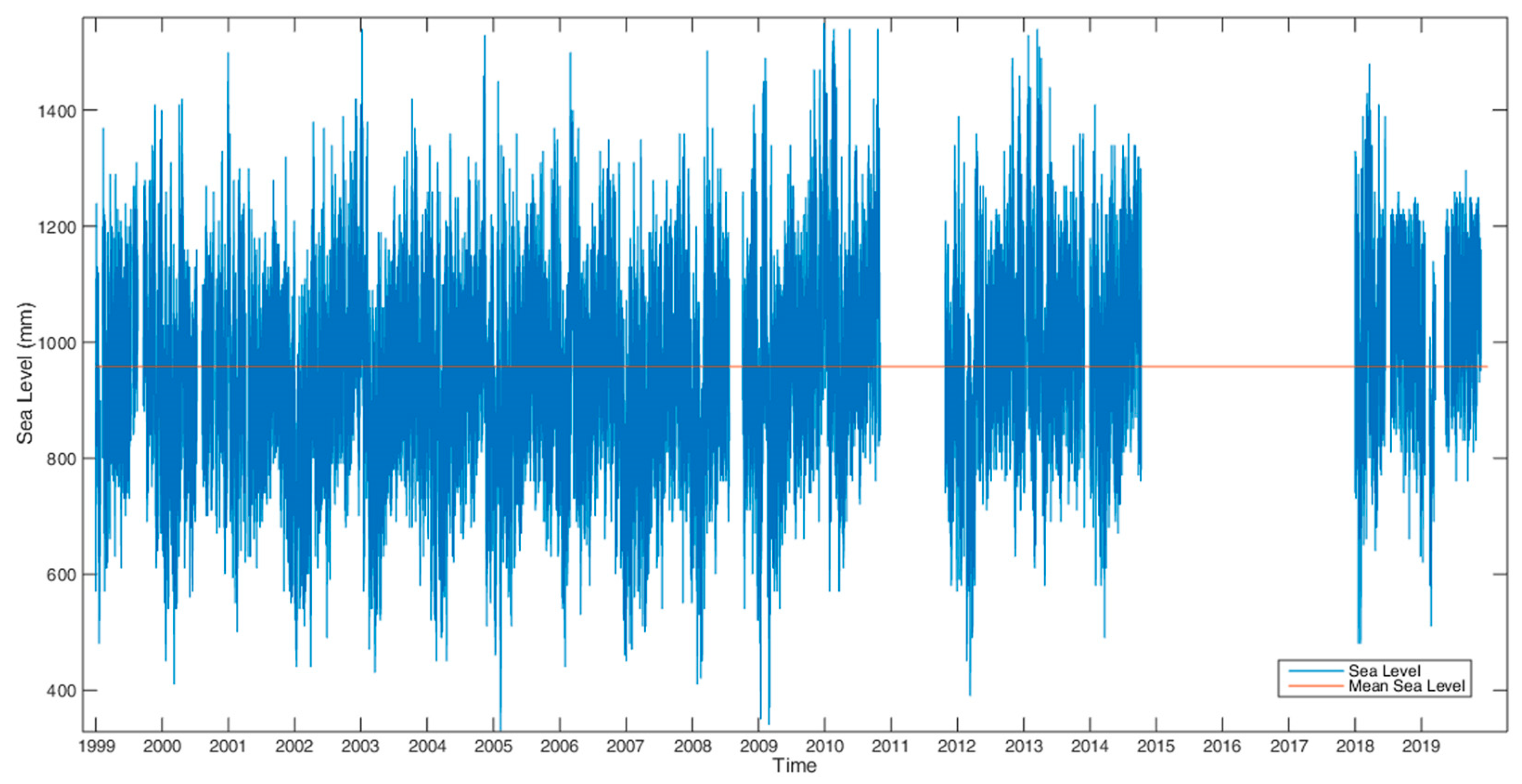
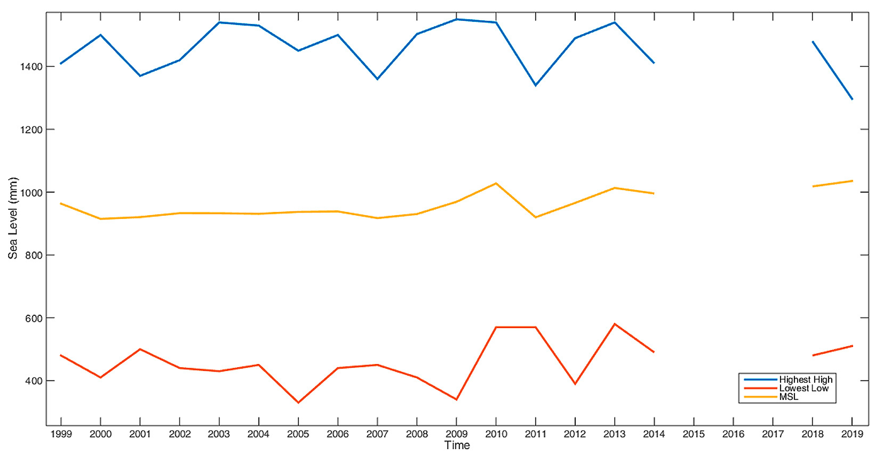
The sea level ranges over 0.8 m for the study period and site (Table 2). As astronomical tide dominates in the total signal, tide prediction has a considerable effect on navigating alongshore and port safety. Harbor and coastal approaches are influenced by sea level. In that context, tide prediction provides the appropriate information for safety in navigation combined with individual ship characteristics. Additionally, the highest highs and the lowest lows are significant values for port establishment and relative infrastructure designs.

In the timespan studied, extreme storm surges over 0.15 m coincide mostly with average sea level observations. Hazardous situations, such as flooding, can occur when both storm surges and tide level exhibit their extremes at the same time. In such circumstances, the sea level behavior and analysis before flooding constitute a crucial parameter as an alarm for hazard prediction. In this regard, the tidal model discussed in this study contributes toward hazard prediction by computing separated sea level components and combining them into a global estimate. Extreme storm surge values have not been extensively studied, as this aspect deviates from the central goal of the current research. Sparse occurrences in the time series of the total sea level signal indicated that there is a need for future investigation of their correlation with other sea level components. An interesting extension of this point would be studying their spatial distribution and correlation, leading to a more comprehensive spatio-temporal analysis of sea level components. This analysis would be helpful in servicing an insight into climate change and its effects on sea level variation, together with coastal design infrastructure at both engineering [52,53] and environmental [8,37] levels.

Regarding the study period, four storm events exhibited surges of some decimeters. In these extreme events, tidal prediction becomes crucial, as it will lead to total sea level estimation. High tidal levels combined with extreme storm surges can lead to flooding at nearby shores. In this regard, high sea levels from astronomical tide predictions paired with weather forecasts accounting for extreme storm surges could trigger alarms for the civil protection of near-shore dwellers.

As a general conclusion, the astronomical tide at the Thessaloniki station is low, and storm surges are even lower. Of course, some extreme values exist and are pointed out. Model residuals, despite their standard deviation values, indicate a small mean value, suggesting a good performance of the model adopted. Also, Willmott Skill and Nash–Sutcliffe efficiency show improved results when storm surges are included in the computations. In conclusion, it is apparent that storm surges contribute significantly to sea level estimation, even if they are low. Therefore, astronomical tide prediction combined with storm surge components can lead to a more accurate sea level estimation. Extreme storm surge events occurring simultaneously with extreme tidal levels could have dangerous consequences for coastal areas. Various damage and even the loss of lives are known in many regions because of that interaction. Recently, the sea level rise observed due to climate change would strengthen this effect, indicating that coastal areas are becoming even more vulnerable. Moreover, storm surges augmented by wave propagation modeling can affect coastal structure design in order to avoid flooding [54].

In reverse, the studies of sea level estimation contribute to climate change studies. Evidently, climate change is responsible for various natural disasters occurring at a global scale, and sea level monitoring is a key parameter contributing to climate change studies. Therefore, consistent analysis and the accurate prediction of sea level variation are key aspects in the design and setup of early warning notes of such phenomena. Additionally, sea level studies contribute to various scientific purposes. Geodesy encompasses sea level studies, as they contribute to height systems and geoid determinations [55,56]. Moreover, accurate determination of tidal signal is critical for satellite altimetry calibration and precise tidal loading estimation for GNSS stations.

Time is a crucial parameter at all scales, and temporal variation is expressed either by the discrete values visualizing a phenomenon (time series) or by a compact function of time (formula). In this study, mean sea level was considered as a constant, which gives it the character of a bias to sea level fluctuations by tide and meteorological conditions. The linear trend added is a rough time-varying parameter. Future analyses should estimate a function for MSL, engaging time as a variable. Under this assumption, MSL stands for the low-frequency signal, astronomical tide is the intermediate one, and storm surge represents the high-frequency part of the total sea level signal. Contrarily, MSL could also be studied at a macroscale level to reveal long-term effects. This also leads to investigating the contributing factors of climate change.

References

1. Gazenave, A.; Bonnefond, P.; Mercier, F.; Dominh, K.; Toumazou, V. Sea level variations in the Mediterranean Sea and Black Sea from satellite altimetry and tide gauges. Glob. Planet. Chang. 2002, 34, 59–86. [Google Scholar] [CrossRef]
2. Barbosa, S.A. Sea Level Change in the North Atlantic from Tide Gauge and Satellite Altimetry. Ph.D. Thesis, Faculdade de Ciensies da Universidade do Porto, Porto, Portugal, 2005. [Google Scholar]
3. Merrifield, M.; Aarup, T.; Allen, A.; Aman, A.; Bradshaw, E.; Caldwell, P.; Fernandes, R.M.S. The Global Sea Level Observing System GLOSS. In Proceedings of the Ocean Information for Society: Sustaining the Benefits, Realizing the Potential, Venice, Italy, 21–25 September 2009. [Google Scholar]
4. Bitharis, S.; Ampatzidis, D.; Pikridas, C.; Fotiou, A.; Schuh, H. The geocentric sea-level rise in the Hellenic area: The synergy of tide-gauges measurements and collocated GNSS stations. In Proceedings of the International Symposium on Gravity, Geoid and Height Systems, Thessaloniki, Greece, 19–23 September 2016. [Google Scholar]
5. Lee, T.C.; Wong, C.F. Historical Storm Surges and Storm Surge Forecasting in Hong Kong. In Proceedings of the JCOMM Scientific and Technical Symposium on Storm Surges (SSS), Seoul, Republic of Korea, 2–6 October 2007. [Google Scholar]
6. Swail, V.; Lee, B.; Soares, A.; Resio, D.; Horsburgh, K.; Murty, T.; Dube, S.; Entel, M.; Flowerdew, J. Storm Surge. In Proceedings of the Ocean Obs ’09: Sustained Ocean Observations and Information for Society, Venice, Italy, 21–25 September 2009; Volume 2. [Google Scholar]
7. Macris, C.; Androulidakis, Y.; Baltikas, V.; Krestenitis, Y. A 37-year analysis of the storm surges in the Mediterranean and Black Seas. In Proceedings of the 12th Panhellenic Symposium of Oceanography & Fisheries, Corfu, Greece, 20 February 2018. [Google Scholar]
8. Luque, P.; Gomez-Pujol, L.; Marcos, M.; Orfila, A. Coastal Flooding in the Balearic Islands During the Twenty-First Century Caused by Sea-Level Rise and Extreme Events. Front. Mar. Sci. 2021, 8, 67452. [Google Scholar] [CrossRef]
9. Nikolaidis, M.; Danezis, C. An initial overview of tidal and sea level variability in Cyprus. In Proceedings of the Eighth International Conference on Remote Sensing and Geoinformation of the Environment (RSCy2020), Paphos, Cyprus, 16–18 March 2020; Volume 11524. [Google Scholar]
10. Mendelsohn, R. Predicting Major Storm Levels. Atmosphere 2021, 12, 756. [Google Scholar] [CrossRef]
11. Andritsanos, V.D.; Arabelos, D.; Spatalas, S.D.; Tziavos, I.N. Mean Sea Level Studies in the Aegean Sea. Phys. Chem. Earth A 2000, 25, 53–56. [Google Scholar] [CrossRef]
12. Hwang, C.; Hsu, H.Y.; Jang, R.J. Global Mean Sea Surface and Marine Gravity Anomaly from Multi-Satellite Altimetry: Applications on Deflection-geoid and Inverse Vening Meinesz Formulae. J. Geod. 2002, 76, 407–418. [Google Scholar] [CrossRef]
13. Hayden, T.; Rangelova, E.; Sideris, M.G.; Veronneau, M. Evaluation of W0 in Canada using tide gauges and GOCE gravity field models. J. Geod. Sci. 2012, 2, 290–301. [Google Scholar] [CrossRef]
14. Woppelmann, G.; Marcos, M. Vertical Land Motion as a Key to Understanding Sea Level Change and Variability. Rev. Geophys. 2016, 54, 64–92. [Google Scholar] [CrossRef]
15. Monitillet, J.-P.; Bos, M.S.; Melbourne, T.I.; Williams, S.D.P.; Fernades, R.M.S.; Szeliga, W.M. Estimation of the Vertical Land Motion from GNSS Time Series and Application in Quantifying Sea-Level Rise. In Geodetic Time Series Analysis in Earth Science; Springer: Cham, Switzerland, 2020; Chapter 11. [Google Scholar]
16. Danezis, C.; Nikolaidis, M.; Mettas, C.; Hadjimitsis, D.; Kokosis, G.; Kleanthous, C. Establishing an Integrated Permanent Sea-Level Monitoring Infrastructure towards the Implementation of Maritime Spatial Planning in Cyprus. J. Mar. Sci. Eng. 2020, 8, 861. [Google Scholar] [CrossRef]
17. Pugh, D.; Woodworth, P. Sea-Level Science: Understanding Tides, Surges, Tsunamis and Mean Sea Level, 2nd ed.; Cambridge University Press: New York, NY, USA, 2014; ISBN 978-1107-02819-7. [Google Scholar]
18. Krestenitis, Y.; Kombiadou, C.; Macris, C.; Androulidakis, Y.; Karambas, V. Coastal Engineering Marine Environmental Hydraulics; Greek Academic Digital Books Kallipos; Greek Association of Academic Libraries, NTUA: Athens, Greece, 2015; ISBN 978-960-603-253-0. [Google Scholar]
19. Boon, J. Secrets of the Tide; Woodhead Publishing: Oxford/Cambridge, UK; Philadelphia, PA, USA; New Delhi, India, 2010; ISBN 978-1-904275-17-6. [Google Scholar]
20. Pugh, D. Tides, Surges and Mean Sea-Level; John Wiley & Sons: Chichester, UK; New York, NY, USA; Brisbane, Australia; Toronto, ON, Canada; Singapore, 1996; ISBN 047191505X. [Google Scholar]
21. Ryabinin, V.; Zilberstein, O.; Seifert, W. Storm Surges; Marine Meteorology and Related Oceanographic Activities; Report No. 33; World Meteorological Organization: Geneva, Switzerland, 1996. [Google Scholar]
22. IOC (Intergovernmental Oceanographic Commission). Manual on Sea Level Measurement and Interpretation; Manuals and Guides 14; UNESCO: Paris, France, 1985. [Google Scholar]
23. Wakelin, S.L.; Woodworth, P.L.; Flather, R.A.; Williams, J.A. Sea-Level Dependence on the NAO Over the NW European Continental Self. Geophys. Res. Lett. 2003, 30, 1403. [Google Scholar] [CrossRef]
24. Tsimplis, M.N.; Alvarez-Fanjul, E.; Gomis, D.; Fenoglio-Marc, L.; Perez, B. Mediterranean Sea Level trends: Atmospheric Pressure and Wind Contribution. Geophys. Res. Lett. 2005, 32, L20602. [Google Scholar] [CrossRef]
25. Tsimplis, M.; Marcos, M.; Colin, J.; Somot, S.; Pascual, A.; Shaw, A.G.P. Sea Level Variability in the Mediterranean Sea During 1990s on the Basis of Two and One 3d model. J. Mar. Syst. 2009, 78, 109–123. [Google Scholar] [CrossRef]
26. Marcos, M.; Tsimplis, M.N. Coastal sea level trends in Southern Europe. Geophys. J. Int. 2008, 175, 70–82. [Google Scholar] [CrossRef]
27. Papadopoulos, A. Measurement Analysis for Sea Level Determination and Satellite Altimetry. Ph.D. Thesis, Technical University of Crete, Chania, Greece, 2009. [Google Scholar]
28. Simav, M.; Yildiz, H.; Turkezer, A.; Lenk, O.; Ozsoy, E. Sea Level Variability at Antalya and Mentes tide gauges in Turkey: Atmospheric, Steric and Land Motion Contributions. Stud. Geophys. Geod. 2012, 56, 215–230. [Google Scholar] [CrossRef]
29. Papazachariou, D. Development of Tidal Model for Mediterranean Sea Assimilating Altimetry and Tidal Data from Tide Gauges in Hydrodynamic Models. Ph.D. Thesis, Polytechnic School, Aristotle University of Thessaloniki, Thessaloniki, Greece, 2013. [Google Scholar]
30. Fer, I.; Muller, M.; Peterson, A.K. Tidal forcing, energetics, and mixing near the Yermak Plateau. Ocean Sci. 2015, 11, 287–304. [Google Scholar] [CrossRef]
31. Gikas, V. Ambient Vibration Monitoring of Slender Structures by Microwave Interferometer Remote Sensing. J. Appl. Geod. 2012, 6, 167–176. [Google Scholar] [CrossRef]
32. García-Molina, P.; Rodríguez-Mediavilla, J.; García-Ripoll, J.J. Quantum Fourier Analysis for Multivariate Functions and Applications to a Class of Schrödinger-type Partial Differential Equations. Phys. Rev. A 2022, 105, 012433. [Google Scholar] [CrossRef]
33. Gikas, V.; Cross, P.A.; Akuamoa, A. A rigorous ans integrated approach to hydrophone and source positioning during multi-streamer offshore seismic exploration. Hydrogr. J. 1995, 77, 11–24. [Google Scholar]
34. Simon, B. Coastal Tides; Institute Oceanographique, Fondation Albert 1er, Prince de Monaco: Monte-Carlo, Monaco, 2013; ISBN 978-2-903581-83-1. [Google Scholar]
35. Georges, K.; Simon, B. The species concordance method of tide prediction in estuaries. Int. Hydrogr. Rev. 1984, 61, 121–146. [Google Scholar]
36. Torres, M.J.; Nadal_Caraballo, N.C. Rapid Tidal Reconstruction with UTide and the ADCIRC Tidal Database; StormSim: Metamodelling of Coastal Storm Hazards for Parabolistic Applications; ERDC SR-21-3; US Army Corps of Engineers, Engineer Research and Development Center: Vicksburg, MS, USA, 2021. [Google Scholar]
37. Hyder, P.; Simpson, J.H.; Christopoulos, S.; Krestenitis, Y. The seasonal cycles of stratification and circulation in the Thermaikos Gulf Region of Freshwater Influence (ROFI), north-west Aegean. Cont. Shelf Res. 2002, 22, 2573–2597. [Google Scholar] [CrossRef]
38. Peng, S.; Li, Y. A parabolic model of drag coefficient for storm surge simulation in the South China Sea. Sci. Rep. 2015, 5, 15496. [Google Scholar] [CrossRef] [PubMed]
39. World Meteorological Organization. Guide to Storm Surge Forecasting, 2011th ed.; No 1076; WMO: Geneva, Switzerland, 2011. [Google Scholar]
40. Hsu, S.A.; Meindl, E.; Gilhousen, D.B. Determining the Power-Law Wind-Profile Exponent under Near-Neutral Stability Conditions at Sea. J. Appl. Meteorol. Climatol. 1994, 33, 757–765. [Google Scholar] [CrossRef]
41. Filom, S.; Radfar, S.; Panahi, R. A comparative study of different wind speed distribution models for accurate evaluation of onshore wind energy potential: A case study on the southern coasts of Iran. Prepr. Eng. 2020. [Google Scholar] [CrossRef]
42. Caldwell, P. Hourly Sea Level Data Processing and Quality Control Software: Update for 64-bit Microsoft Operating Systems. SLP64 User Manual (Version 4.0); JIMAR Contribution No. 14-389; Joint Archive for Sea Level of the National Oceanographic Data Center and University of Hawaii Sea Level Center: Seattle, HI, USA, 2014. [Google Scholar]
43. Codiga, D.L. Unified Tidal Analysis and Prediction Using the UTide Matlab Functions; Technical Report 2011-01; Graduate School of Oceanography, University of Rhode Island: Narragansett, RI, USA, 2011; p. 59. [Google Scholar] [CrossRef]
44. Lefler, K.E.; Jay, D.A. Enhancing tidal harmonic analysis: Robust (hubrid L-1/L-2) solution. Cont. Shelf Res. 2009, 29, 78–88. [Google Scholar] [CrossRef]
45. Conte, D.; Lionello, P. Characteristics of large positive and negative surges in the Mediterranean Sea and their attenuation in future climate scenarios. Glob. Planet. Chang. 2013, 111, 159–173. [Google Scholar] [CrossRef]
46. Foreman, M.G.G. Manual for Tidal Heights Analysis and Prediction. In Pacific Marine Science Report 77-10; Institute of Ocean Sciences: Sidney, BC, Canada, 1977; (Revised 2004). [Google Scholar]
47. Tsimiplis, M.N.; Procor, R.; Flather, R.A. A two-dimensional tidal modelling for the Mediterranean. J. Geophys. Res. 1995, 100, 16223–16239. [Google Scholar] [CrossRef]
48. Peng, S.; Li, Y.; Xie, L. Adjusting the wind stress drag coefficient in storm surge forecasting using an adjoint technique. J. Atmos. Ocean. Technol. 2012, 30, 590–608. [Google Scholar] [CrossRef]
49. Marcos, M.; Tsimplis, M.N.; Shaw, A.G.P. Sea level extremes in Southern Europe. J. Geophys. Res. 2009, 114, C01007. [Google Scholar] [CrossRef]
50. de Vries, H.; Breton, M.; de Mulder, T.; Krestenitis, Y.; Ozer, J.; Proctor, R.; Ruddick, K.; Salomon, J.C.; Voorrips, A. A comparison of 2D storm surge models applied to three shallow European seas. Environ. Softw. 1995, 10, 23–42. [Google Scholar] [CrossRef]
51. Sampurno, J.; Vallaeys, V.; Ardianto, R.; Hanert, E. Modelling interactions between tides, storm surges, and river discharges in the Kapuas River delta. Biogeosciences 2022, 19, 2741–2757. [Google Scholar] [CrossRef]
52. Radfar, S.; Shafieegar, M.; Akbari, H. Impact of copula model selection on reliability-based design optimization of a rubble mound breakwater. Ocean. Eng. 2022, 260, 112023. [Google Scholar] [CrossRef]
53. Radfar, S.; Shafieefar, M.; Akbari, H.; Galiatsatou, P.A.; Mazyak, A.R. Design of a rubble mound breakwater under the combined effect of wave heght and water levels, under present and future conditions. Appl. Ocean. Res. 2021, 112, 102711. [Google Scholar] [CrossRef]
54. Samaras, A.G.; Karambas, T.V. Modelling the Impact of Climate Change on Coastal Flooding: Implications for Coastal Structures. J. Mar. Sci. Eng. 2021, 9, 1008. [Google Scholar] [CrossRef]
55. Gikas, V.; Mpimis, A.; Androulakis, A. Proposal for Geoid Model Evaluation from GNSS-INS/Leveling Data: Case Study along a Railway Line in Greece. J. Surv. Eng. 2013, 139, 104–139. [Google Scholar] [CrossRef]
56. Varbla, S.; Agren, J.; Ellmann, A.; Poutanen, M. Treatment of Tide Gauge Time Series and Marine GNSS Measurements for Vertical Land Motion with Relevance to the Implementation of the Baltic Sea Chart Datum 2000. Remote Sens. 2022, 14, 920. [Google Scholar] [CrossRef]
Figure 1. An average skew surge in the study area observed in 2009 on the 3rd of November at 03:00 (time of the high tide). It has an amplitude of 65.2 mm and a time shift dt = −1 h. A large one follows at 15:00.
Jmse 11 02033 g001
Figure 2. Quality control and data analysis workflow for sea level estimation.
Jmse 11 02033 g002
Figure 3. Tide gauge (green dot) and meteorological station (red star) locations in the Thessaloniki area.
Jmse 11 02033 g003
Figure 4. Broader Thermaikos Gulf (170 km length) and tide gauge and meteorological station locations in the Thessaloniki area.
Jmse 11 02033 g004
Figure 5. Sea level observations at the Thessaloniki tide gauge and their mean value (red line).
Jmse 11 02033 g005
Figure 6. Statistics of the mean sea level (MSL), the lowest lows (LLs), the highest highs (HHs), and the range (HH-LL) of values at the Thessaloniki tide gauge computed for the entire test period, 1999–2019.
Jmse 11 02033 g006
Figure 7. Mean sea level (MSL), lowest lows (LLs), and highest highs (HHs) observed annually at the Thessaloniki tide gauge for the time period 1999–2019.
Jmse 11 02033 g007
Figure 8. Wind direction and speed at the Thessaloniki Meteorological Station for the time period 1999–2019.
Jmse 11 02033 g008
Figure 9. Time shift correction. Tide prediction using slp64 (red line), observed values (blue line), time-corrected (yellow line) data due to time shift, and corresponding residuals before time correction (purple line) (1–12 August 2003). High residual values from August 1 to 5 reveal a time shift in observations. Note that after the gap on August 5, residuals are smaller, and the prediction better matches the observations.
Jmse 11 02033 g009
Figure 10. Annual astronomical tide prediction for the time period 1999–2019.
Jmse 11 02033 g010
Figure 11. Annual tidal residuals for the time period 1999–2019.
Jmse 11 02033 g011
Figure 12. Frequency distribution of skew surges over 181 mm (mean + std) at the Thessaloniki tide gauge station for the time period 1999–2019. Each column label presents the maximum value in mm.
Jmse 11 02033 g012
Figure 13. Sea level values by tide gauge measurements (blue line), model sea level values (red line), and the corresponding residuals (yellow line) at the Thessaloniki tide gauge station for the time period 1999–2019.
Jmse 11 02033 g013
Figure 14. Tide gauge records (blue line top) vs. calculated storm surges (red line) vs. wind velocity (blue line bottom) for the total timespan (1999–2019), showing their direct correlation.
Jmse 11 02033 g014