
Results of the Study of Resonant Oscillations in the Northern Part of the Shelf of the Peter the Great Gulf, the Sea of Japan

 ,
,  , , ,
, , , 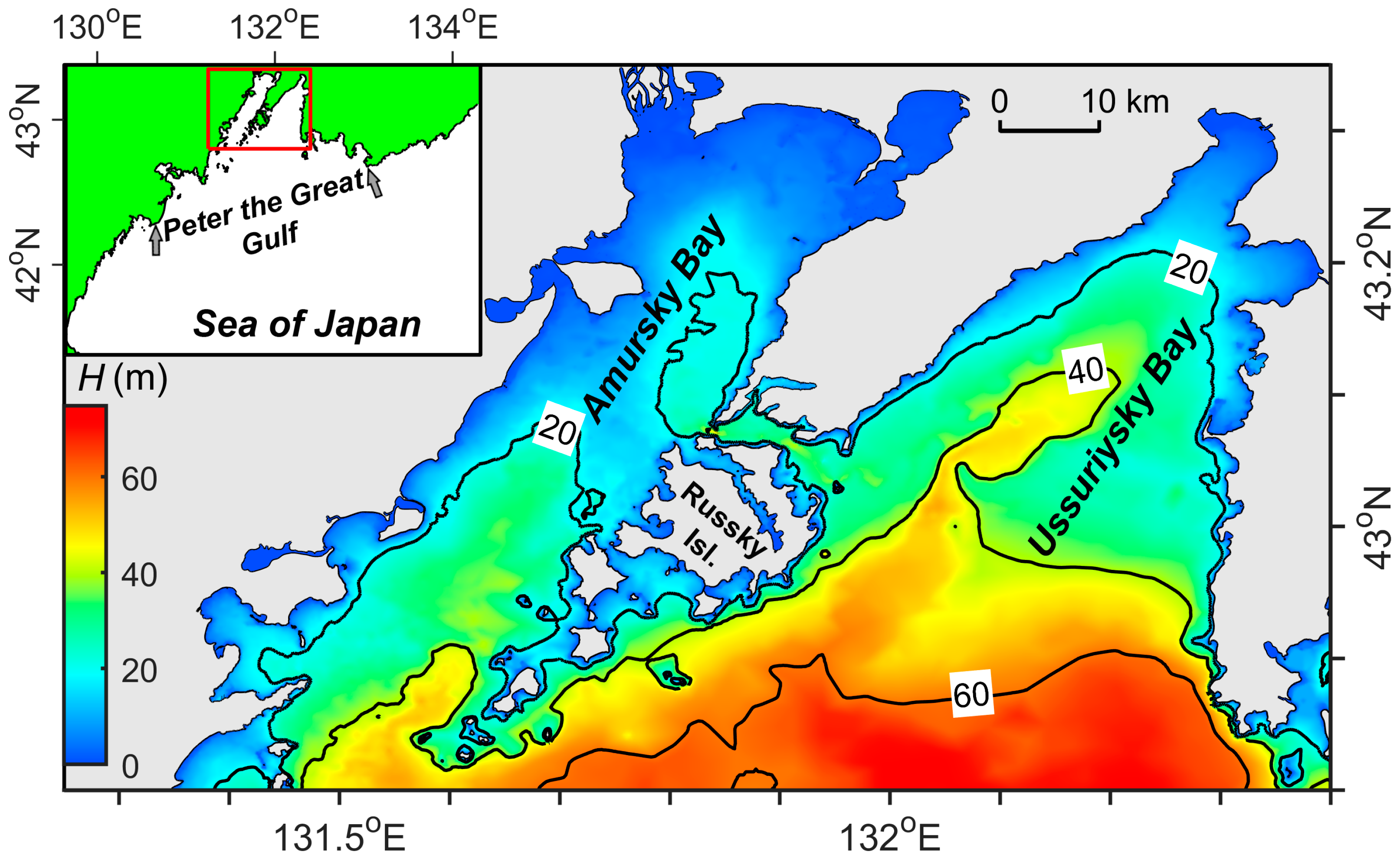
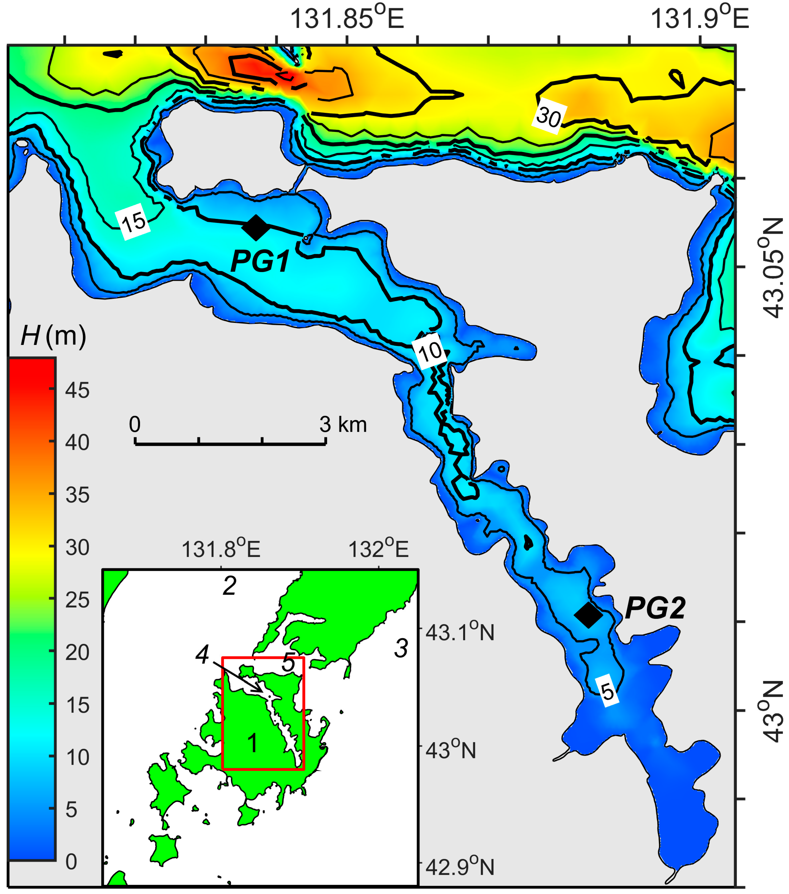
Abstract
:1. Introduction
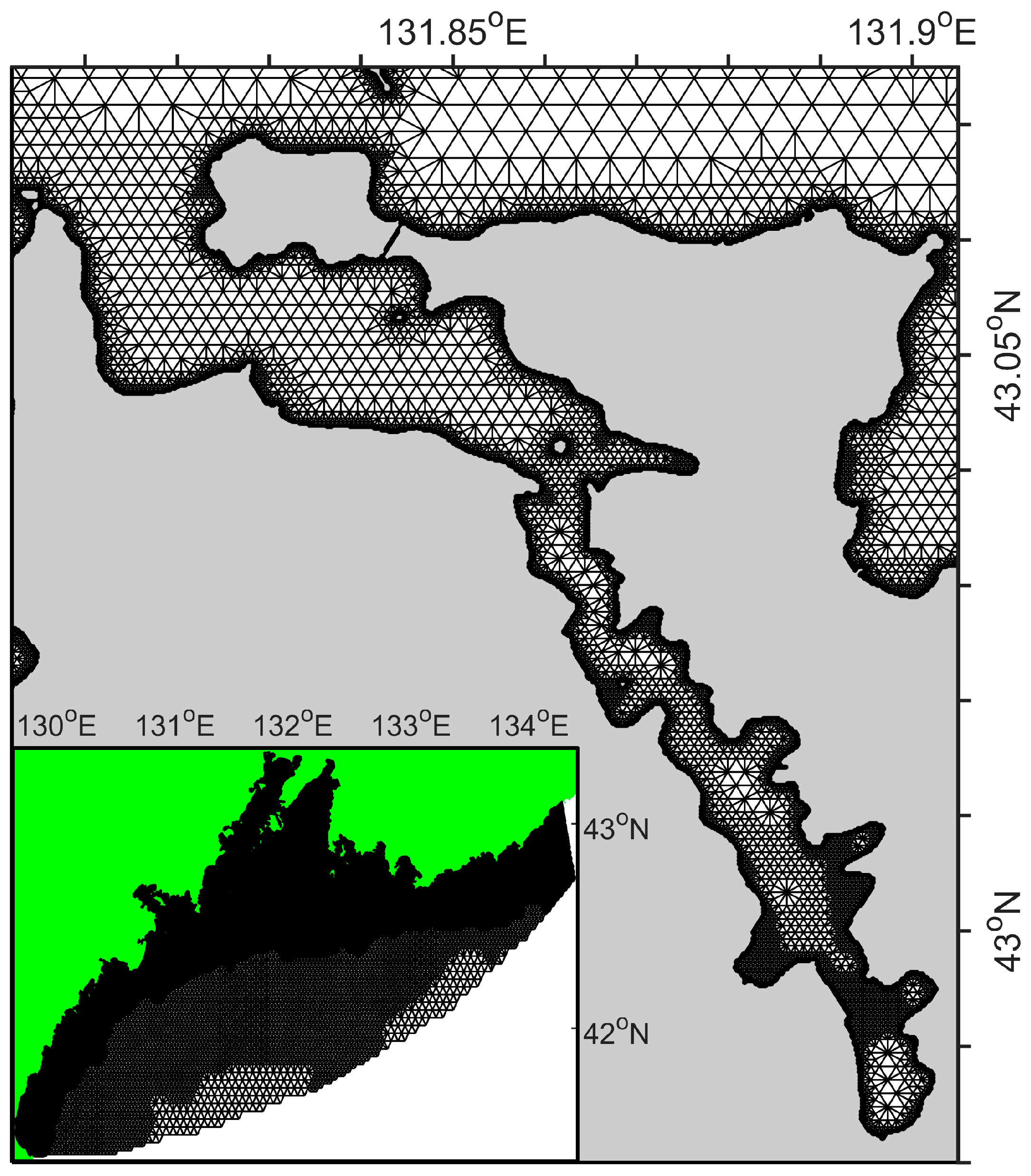
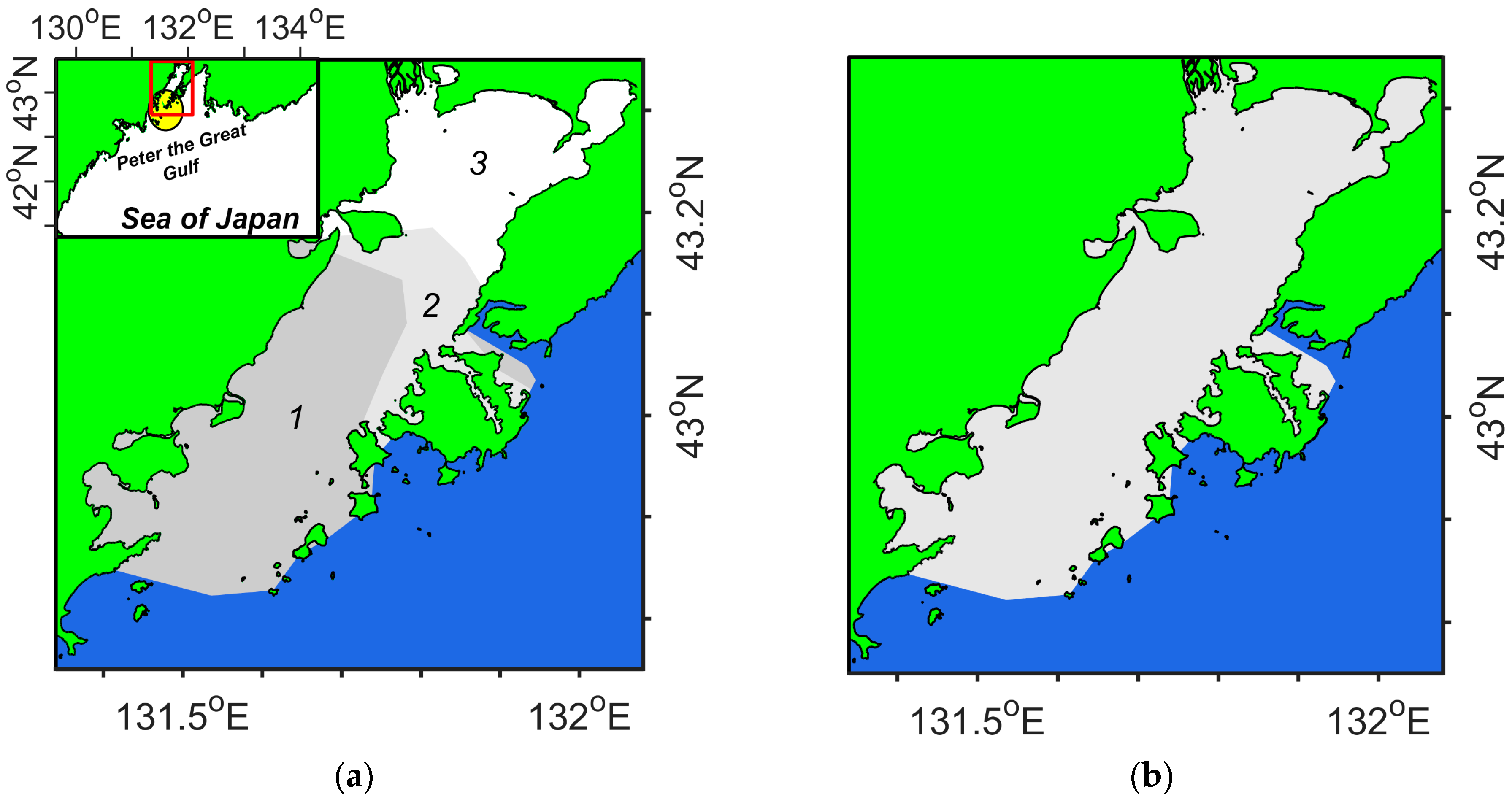
2. Materials and Methods
2.1. In Situ Measurements
2.2. Spectral-Difference Model
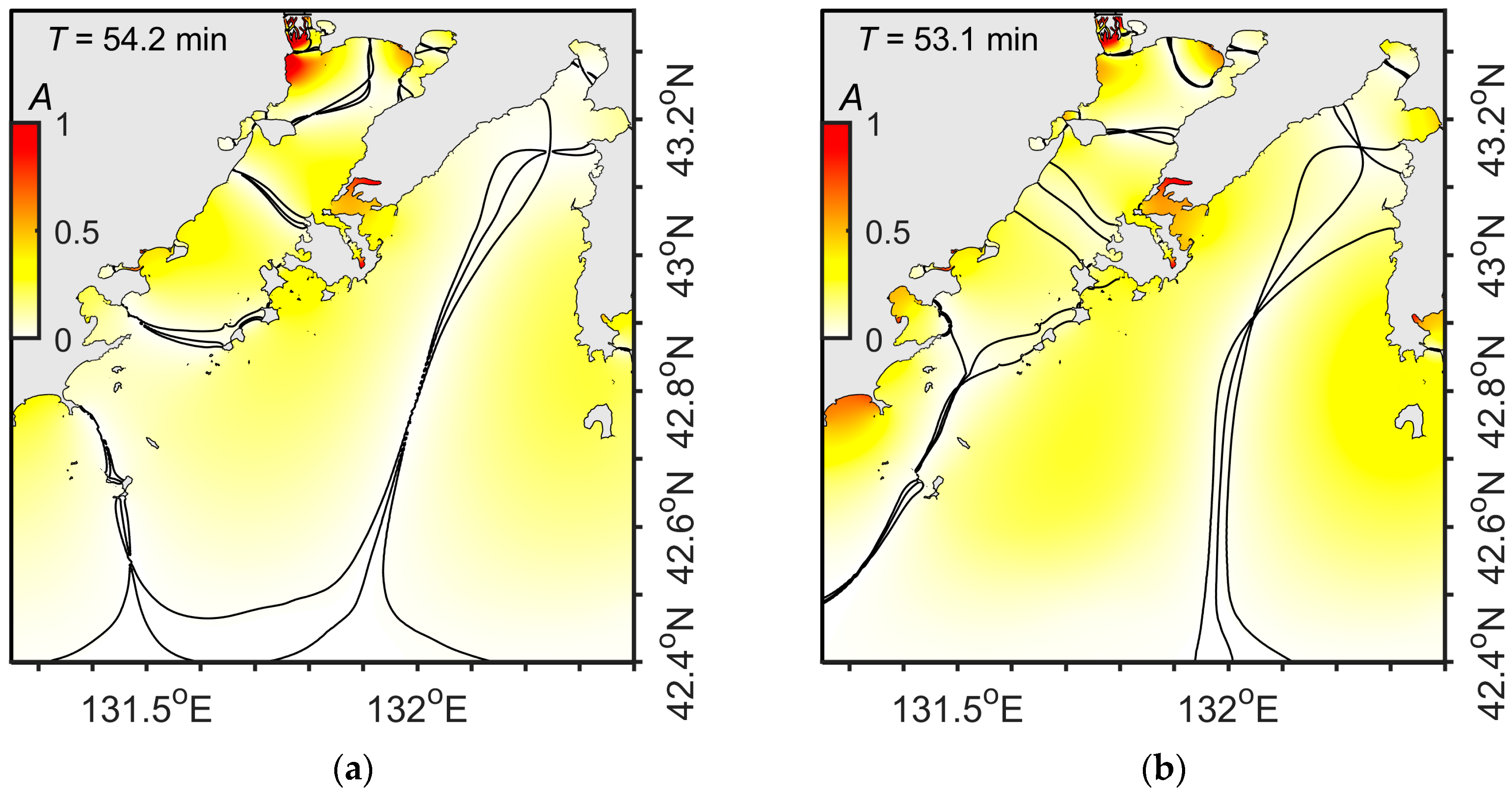
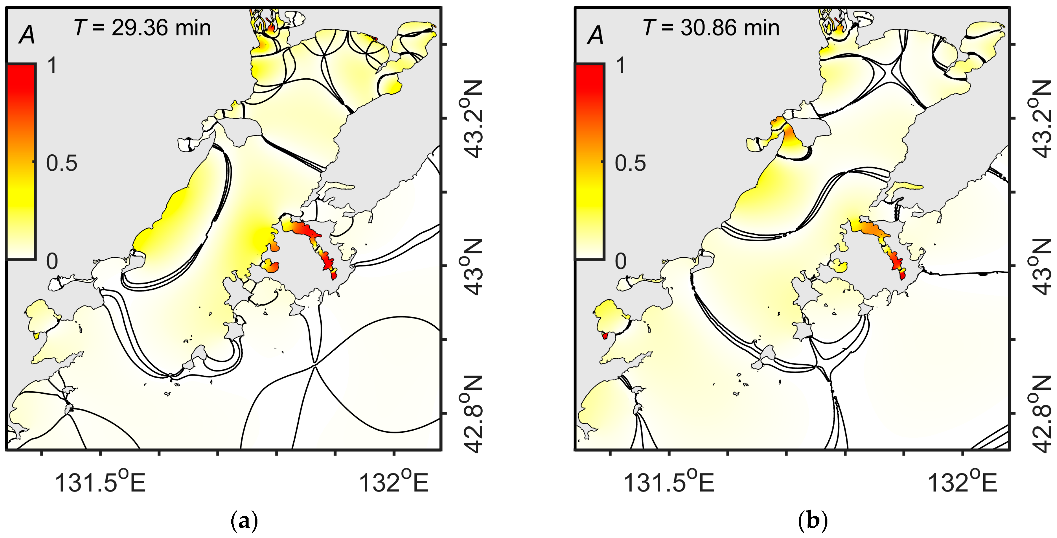
3. Results
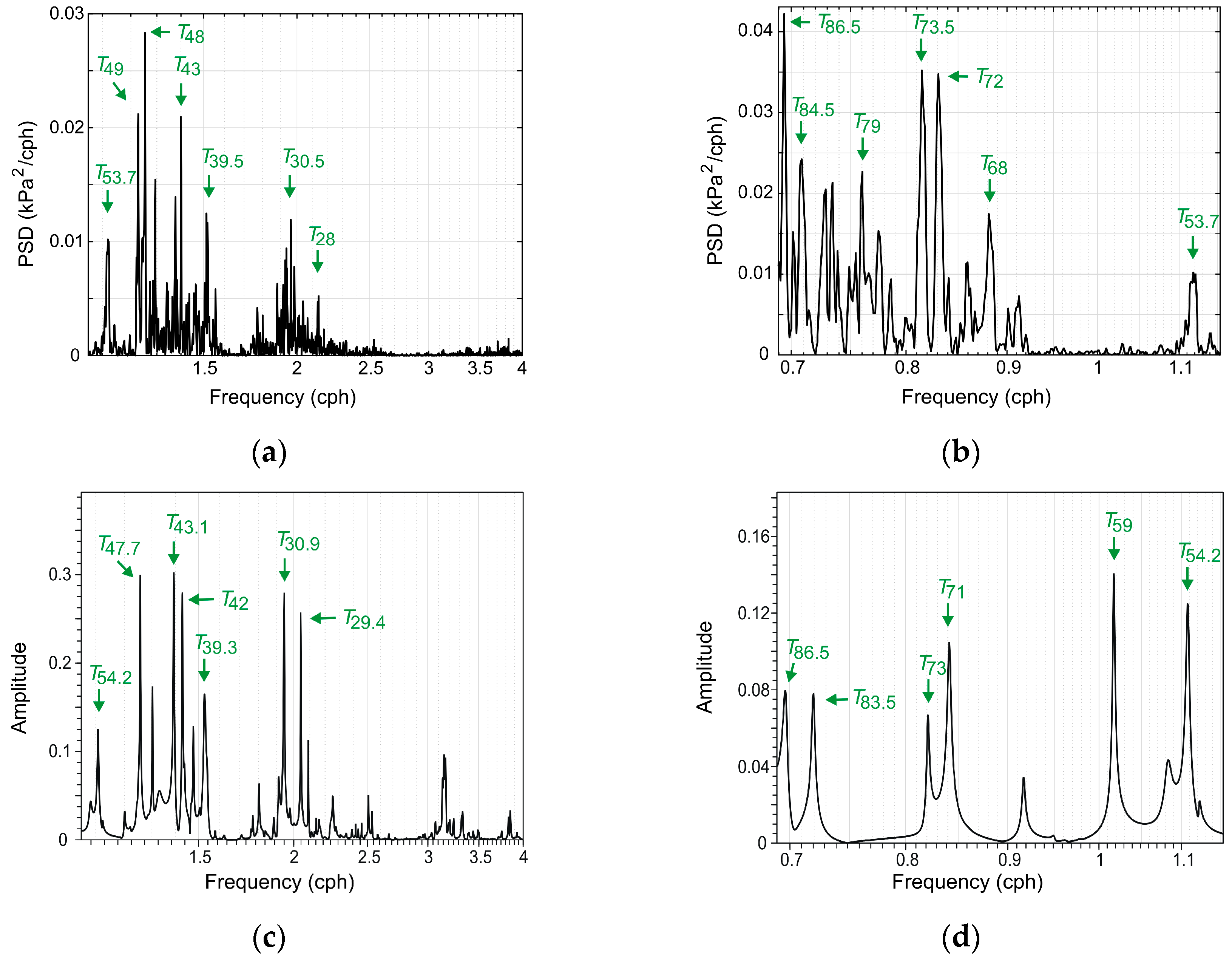
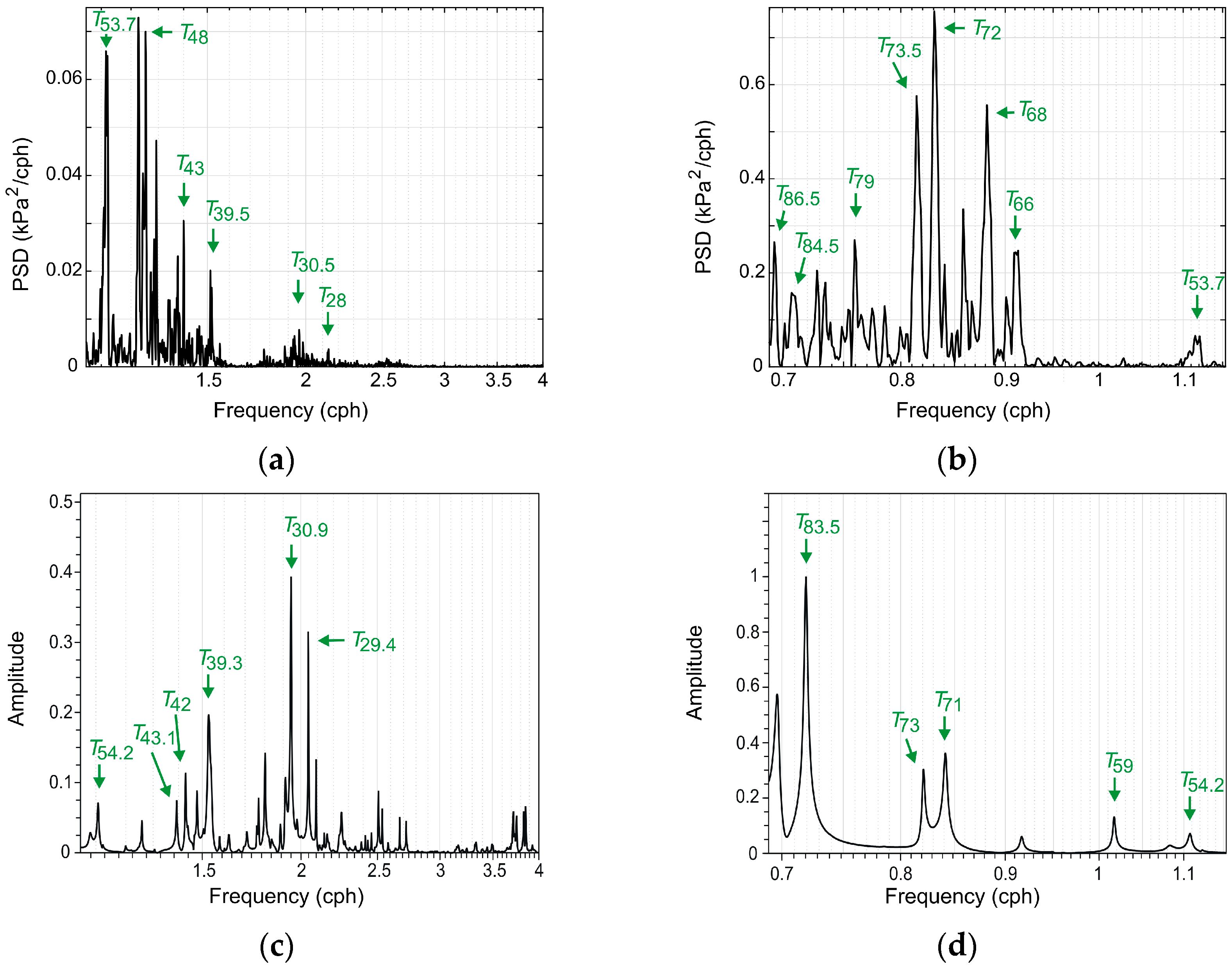
3.1. In Situ Measurements
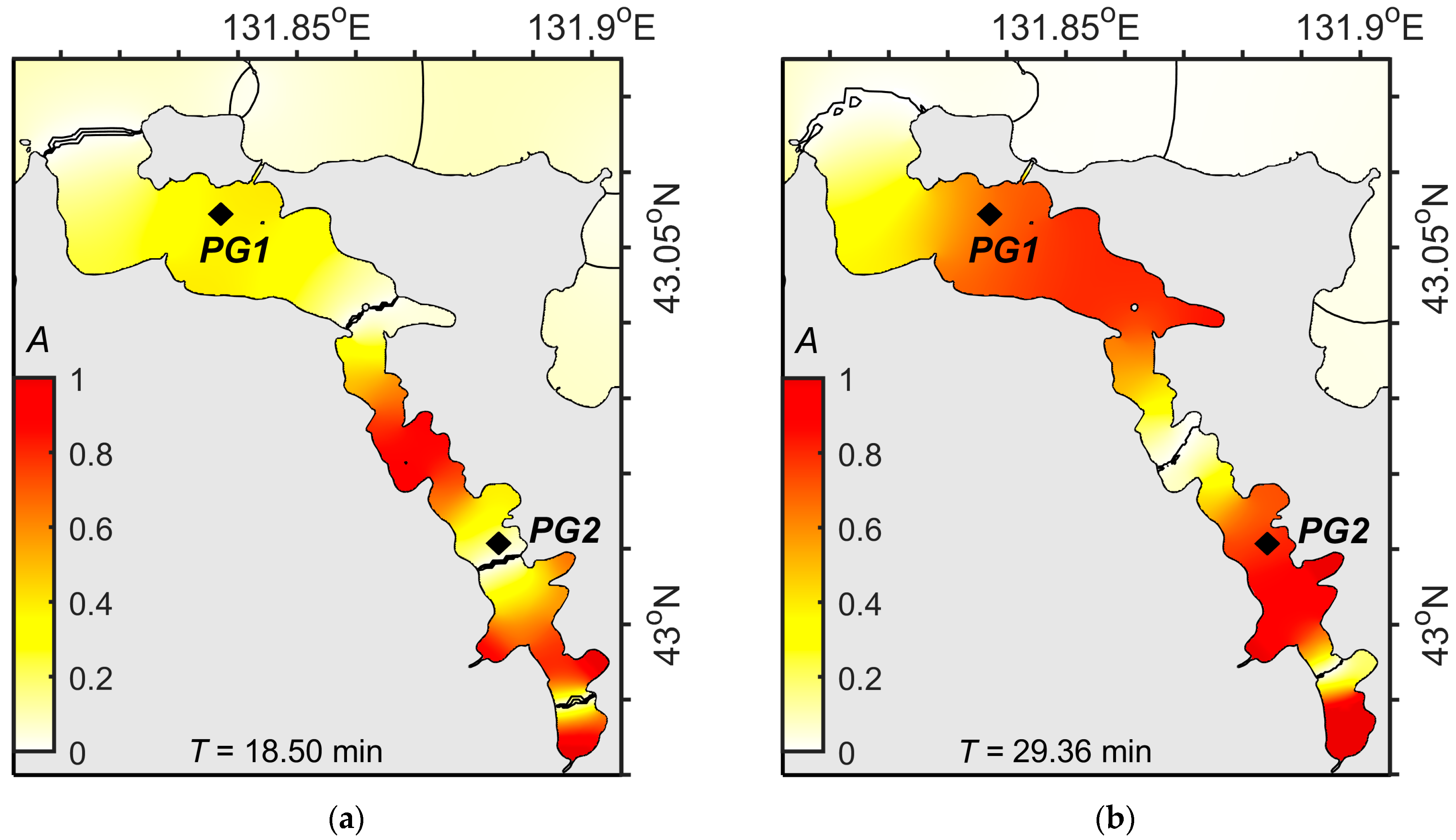
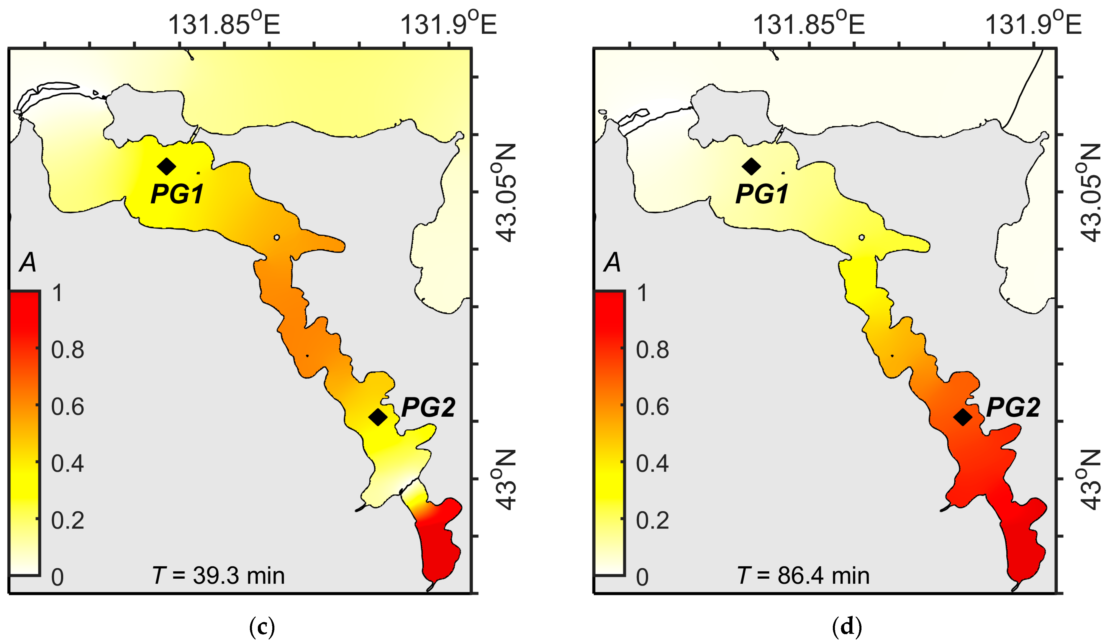
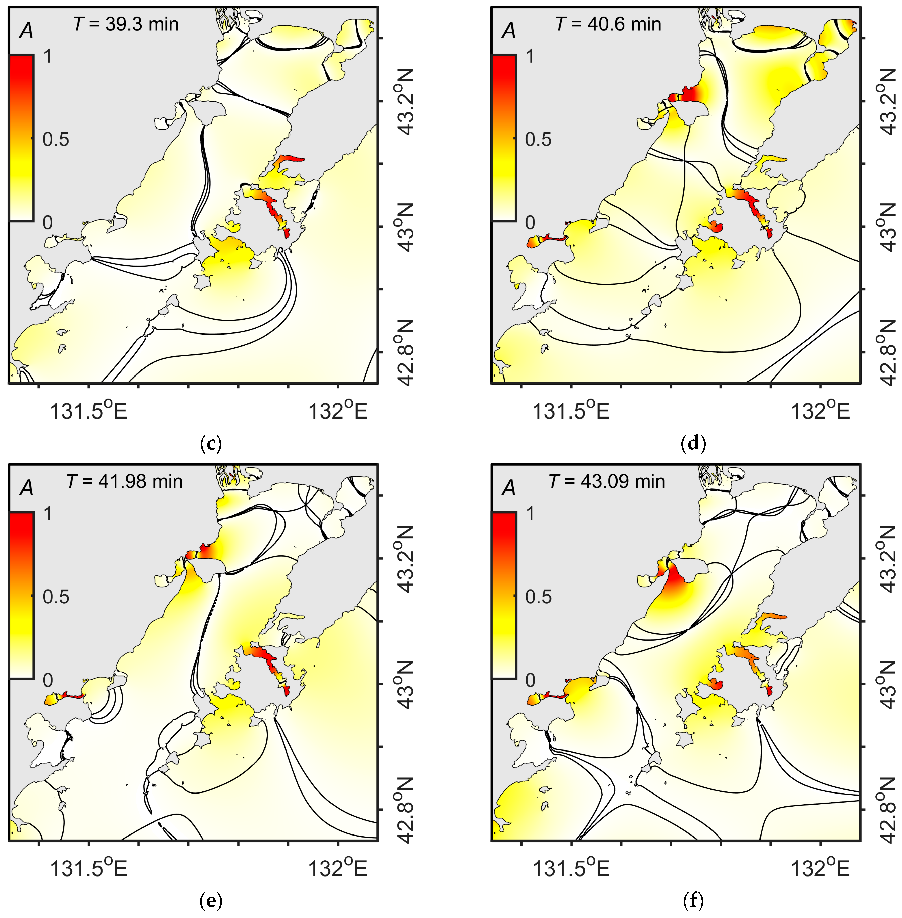
3.2. Results of Numerical Modeling
4. Discussion
5. Conclusions
Author Contributions
Funding
Institutional Review Board Statement
Informed Consent Statement
Data Availability Statement
Acknowledgments
Conflicts of Interest
References
- Rabinovich, A.B. Seiches and Harbor oscillations. In Handbook of Coastal and Ocean Engineering; Chapter 9; Kim, Y.C., Ed.; World Scientific Publishing: Singapore, 2009; pp. 193–236. [Google Scholar]
- Kânoğlu, U.; Okal, E.A.; Baptista, M.A.; Rabinovich, A.B. Introduction to “Sixty Years of Modern Tsunami Science, Volume 1: Lessons and Progress”. Pure Appl. Geophys. 2021, 178, 4689–4695. [Google Scholar] [CrossRef]
- Kânoğlu, U.; Rabinovich, A.B.; Okal, E.A.; Pattiaratchi, C.; Baptista, M.A.; Zamora, N.; Catalán, P.A. Introduction to “Sixty Years of Modern Tsunami Science, Volume 2: Challenges”. Pure Appl. Geophys. 2023, 180, 1541–1547. [Google Scholar] [CrossRef] [PubMed]
- Vilibić, I.; Rabinovich, A.B.; Anderson, E.J. Special issue on the global perspective on meteotsunami science: Editorial. Nat. Hazards 2021, 106, 1087–1104. [Google Scholar] [CrossRef]
- Defant, A. Physical Oceanography; Pergamon Press: London, UK; New York, NY, USA, 1961; Volume 2. [Google Scholar]
- Gao, J.; Ji, C.; Liu, Y.; Ma, X.; Gaidai, O. Influence of offshore topography on the amplification of infragravity oscillations within a harbor. Appl. Ocean Res. 2017, 65, 129–141. [Google Scholar] [CrossRef]
- Gao, J.; Zhou, X.; Zang, J.; Chen, Q.; Zhou, L. Influence of offshore fringing reefs on infragravity period oscillations within a harbor. Ocean Eng. 2018, 158, 286–298. [Google Scholar] [CrossRef]
- Medvedev, I.P.; Vilibić, I.; Rabinovich, A.B. Tidal resonance in the Adriatic Sea: Observational evidence. J. Geophys. Res. Oceans 2020, 125, e2020JC016168. [Google Scholar] [CrossRef]
- Polyakova, A.M. Dangerous and Especially Dangerous Hydrometeorological Phenomena in the North Pacific and Tsunami Waves Near the Primorye Coast; Dalnauka: Vladivostok, Russia, 2012. (In Russian) [Google Scholar]
- Dolgikh, G.I.; Dolgikh, S.G.; Smirnov, S.V.; Chupin, V.A.; Shvets, V.A.; Yakovenko, S.V. Infrasound oscillations in the Sea of Japan. Dokl. Earth Sci. 2011, 441, 1529–1532. [Google Scholar] [CrossRef]
- Smirnov, S.V.; Yaroshchuk, I.O.; Leontyev, A.P.; Shvyrev, A.N.; Pivovarov, A.A.; Samchenko, A.N. Studying resonance oscillations in the eastern part of the Posyet Bay. Russ. Meteorol. Hydrol. 2018, 43, 88–94. [Google Scholar] [CrossRef]
- Smirnov, S.V.; Yaroshchuk, I.O.; Shvyrev, A.N.; Kosheleva, A.V.; Pivovarov, A.A.; Samchenko, A.N. Resonant oscillations in the western part of the Peter the Great Gulf in the Sea of Japan. Nat. Hazards 2021, 106, 1729–1745. [Google Scholar] [CrossRef]
- Chupin, V.; Dolgikh, G.; Dolgikh, S.; Smirnov, S. Study of Free Oscillations of Bays in the Northwestern Part of Posyet Bay. J. Mar. Sci. Eng. 2022, 10, 1005. [Google Scholar] [CrossRef]
- Smirnov, S.V. On calculation of seiche oscillations of the middle part of the Peter the Great Gulf. Numer. Analys. Appl. 2014, 7, 168–179. [Google Scholar] [CrossRef]
- Smirnov, S.V. Seiche Oscillations in the Nakhodka Gulf. Russ. Meteorol. Hydrol. 2016, 41, 57–62. [Google Scholar] [CrossRef]
- Lazaryuk, A.Y.; Kilmatov, T.R.; Marina, E.N.; Kustova, E.V. Seasonal features of the Novik Bay hydrological regime (Russky Island, Peter the Great Bay, Sea of Japan). Phys. Oceanogr. 2021, 28, 632–646. [Google Scholar] [CrossRef]
- Leontyev, A.P.; Yaroshchuk, I.O.; Smirnov, S.V.; Kosheleva, A.V.; Pivovarov, A.A.; Samchenko, A.N.; Shvyrev, A.N. A spatially distributed measuring complex for monitoring hydrophysical processes on the ocean shelf. Instrum. Exp. Technol. 2017, 60, 130–136. [Google Scholar] [CrossRef]
- Thomson, R.E.; Emery, W.J. Data Analysis Methods in Physical Oceanography, 3rd ed.; Elsevier Science: New York, NY, USA, 2014; 728p. [Google Scholar] [CrossRef]
- Flather, R.A. A numerical model investigation of the storm surge of 31 January and 1 February 1953 in the North Sea. Quart. J. R. Met. Soc. 1984, 110, 591–612. [Google Scholar] [CrossRef]
- Chen, C.; Beardsley, R.; Cowles, G.; Qi, J.; Lai, Z.; Gao, G.; Stuebe, D.; Liu, H.; Xu, Q.; Xue, P.; et al. An Unstructured Grid, Finite-Volume Community Ocean Model FVCOM User Manual; SMAST UMASSD Technical Report-13-0701; University of Massachusetts-Dartmouth: North Dartmouth, MA, USA, 2013. [Google Scholar]
- Demmel, J.W.; Gilbert, J.R.; Li, X.S. An asynchronous parallel supernodal algorithm for sparse gaussian elimination. SIAM J. Matrix Anal. Appl. 1999, 20, 915–952. [Google Scholar] [CrossRef]
- Atlas of Peter the Great Gulf and Northwestern Coast of the Sea of Japan to Sokolovskaya Bay (for Small-Size Vessels); Gidrograficheskaya Sluzhba KTOF: Vladivostok, Russia, 2003; p. 10. (In Russian)
- GEBCO Bathymetric Compilation Group. The GEBCO_2020 Grid—A Continuous Terrain Model of the Global Oceans and Land; British Oceanographic Data Centre, National Oceanography Centre, NERC: Swindon, UK, 2020. [Google Scholar] [CrossRef]
- Mesinger, F.; Arakawa, A. Numerical Methods Used in Atmospheric Models; GARP Publication Series No. 17; WMO: Geneva, Switzerland, 1976; p. 64. [Google Scholar]


Disclaimer/Publisher’s Note: The statements, opinions and data contained in all publications are solely those of the individual author(s) and contributor(s) and not of MDPI and/or the editor(s). MDPI and/or the editor(s) disclaim responsibility for any injury to people or property resulting from any ideas, methods, instructions or products referred to in the content. |
© 2023 by the authors. Licensee MDPI, Basel, Switzerland. This article is an open access article distributed under the terms and conditions of the Creative Commons Attribution (CC BY) license (https://creativecommons.org/licenses/by/4.0/).
Share and Cite
Smirnov, S.; Dolgikh, G.; Yaroshchuk, I.; Lazaryuk, A.; Kosheleva, A.; Shvyrev, A.; Pivovarov, A.; Samchenko, A. Results of the Study of Resonant Oscillations in the Northern Part of the Shelf of the Peter the Great Gulf, the Sea of Japan. J. Mar. Sci. Eng. 2023, 11, 1973. https://doi.org/10.3390/jmse11101973
Smirnov S, Dolgikh G, Yaroshchuk I, Lazaryuk A, Kosheleva A, Shvyrev A, Pivovarov A, Samchenko A. Results of the Study of Resonant Oscillations in the Northern Part of the Shelf of the Peter the Great Gulf, the Sea of Japan. Journal of Marine Science and Engineering. 2023; 11(10):1973. https://doi.org/10.3390/jmse11101973
Chicago/Turabian StyleSmirnov, Sergey, Grigory Dolgikh, Igor Yaroshchuk, Alexander Lazaryuk, Alexandra Kosheleva, Alex Shvyrev, Alexander Pivovarov, and Aleksandr Samchenko. 2023. "Results of the Study of Resonant Oscillations in the Northern Part of the Shelf of the Peter the Great Gulf, the Sea of Japan" Journal of Marine Science and Engineering 11, no. 10: 1973. https://doi.org/10.3390/jmse11101973
APA StyleSmirnov, S., Dolgikh, G., Yaroshchuk, I., Lazaryuk, A., Kosheleva, A., Shvyrev, A., Pivovarov, A., & Samchenko, A. (2023). Results of the Study of Resonant Oscillations in the Northern Part of the Shelf of the Peter the Great Gulf, the Sea of Japan. Journal of Marine Science and Engineering, 11(10), 1973. https://doi.org/10.3390/jmse11101973