Article

A Preliminary Study of Suspended Matters Variation Associated with Hypoxia and Shoaling Internal Tides on the Continental Shelf of the Northern Andaman Sea

State Key Laboratory of Satellite Ocean Environment Dynamics, Second Institute of Oceanography, Ministry of Natural Resources, Hangzhou 310012, China
*
Author to whom correspondence should be addressed.
J. Mar. Sci. Eng. 2023, 11(10), 1950; https://doi.org/10.3390/jmse11101950
Submission received: 29 August 2023 / Revised: 25 September 2023 / Accepted: 4 October 2023 / Published: 10 October 2023

Abstract

:
The northern Andaman Sea (AS) continental shelf is unique due to the diverse marine ecosystem and existences of both hypoxia and internal tides, but limited in situ observations restrict our understanding of the hydrographic dynamic process. Based on the turbidity, mean volumes of backscattering strength (MVBS), we qualitatively studied the mean distribution characteristics and temporal variation in suspended matters on the northern AS continental shelf and their relation to hypoxia and internal tides. The results of both MVBS and turbidity revealed that the suspended matters exhibited a three-layer vertical structure. The upper and lower layers exhibited high values, while the middle layer had low values. The upper boundary of the high-value region in the upper layer descended below the surface to a depth of 30 m after sunrise and returned to the surface after sunset, indicating a diel vertical migration of zooplankton and micronekton. Daytime migration depth was likely constrained by hypoxia’s upper boundary. In the lower layer, three MVBS enhancements and attenuations correlated with vertical upward and downward velocities, respectively, primarily driven by uplift or suppression. We proposed vertical velocity patterns resulted from internal bores, possibly triggered by shoaling semidiurnal internal tides.

1. Introduction

The study of the distribution and dynamics of suspended matters is crucial for understanding sediment dynamics and the migration patterns of marine organisms [1,2,3,4]. Typically, high concentrations of suspended matters are found near the sea surface and bottom in coastal areas [5]. The distribution of highly concentrated suspended matters near the surface is primarily influenced by biological activity, while the high concentration near the seabed is caused by sediment resuspension and downslope turbidity currents [6,7]. The thickness and position of highly concentrated suspended matters vary over time and depend on local hydrodynamic conditions, such as oxygen distribution, thermocline, and internal waves [8,9]. The horizontal and vertical movement of highly concentrated suspended matters, which contain nutrients, carbon, iron, and other minerals from land, play a crucial role in maintaining ecosystems on the continental shelf [10].
The water in the near-surface layer contains a high concentration of suspended matters, which includes a rich variety of marine organisms. The variations in suspended matters are influenced by both light and oceanic conditions [11,12]. The vertical migration of zooplankton and micronekton in the near-surface layer is primarily driven by changes in light intensity [13]. Numerous studies have indicated that marine organisms migrate vertically to the upper layer to forage at night and retreat to the deeper layer to avoid predation and harm from ultraviolet exposure during the day [13,14]. As a result, intensified mean volume backscattering strength (MVBS), which can be transformed from Acoustic Doppler Current Profiler (ADCP) echoes and is directly related to the concentration of suspended matters, has been observed at different depths in the upper ocean during day and night [3,4,15]. Additionally, among the various environmental factors, dissolved oxygen concentrations ([DO]s) are considered a crucial indicator of the vertical migration depth for marine organisms [8]. Generally, the formation of hypoxia (where [DO]s < 2.0 mg L−1) is associated with factors such as high rates of primary production, extended residence times of bottom water, stratification, and continental shelf topography [16,17]. The impact of hypoxia on the vertical movement of organisms varies among different species [15,18]. Organisms employ various strategies to cope with the hypoxic environment, including reducing their habitats to avoid hypoxia or performing diel vertical migration towards the upper layer of the hypoxic zone [19].
Internal tides, one of the most important internal waves, are an essential component of the ocean dynamics in the continental slope regions. They are generated in stratified waters by the interaction of tidal currents with bottom topography, such as mid-ocean ridges, seamounts, and continental shelves [20]. When the cyclic, back-and-forth tidal currents interact with the bottom topography, the disturbances in water depth cause fluctuations in the isopycnals. Internal tides originate at the bottom topography and subsequently propagate away from it. When diurnal (semidiurnal) tidal currents pass over the topography, diurnal (semidiurnal) internal tides are generated, with a period of approximately 24 (12) h. As internal tides propagate across the continental slope, nonlinear internal waves, including internal bores and internal solitary waves, may evolve from them. Internal tides are responsible for the resuspension and transportation of sediments on the seabed. The occurrence of sediment resuspension triggered by internal tides has been observed and studied in various areas, including the South China Sea [21], Otsuchi Bay in Japan [1], the northern shelf of Portugal [22], the Oregon shelf of the United States [23], and the California shelf [24]. The resuspension of sediments induced by internal waves is not only influenced by the horizontal shear of the current but is also facilitated by the vertical velocities [25]. Additionally, the mixing and transport induced by internal wave breaking have been experimentally verified in laboratory settings [26,27]. Both numerical simulation and observation have shown that shoaling internal tides suspended seabed sediments through horizontal velocity within the vortex and horizontal shear of the current. Subsequently, the sediments are entrained into the water column by vertical velocities, resulting in a highly concentrated suspended matter layer [28,29,30]. This highly concentrated suspended matters water near the seabed separates from the slope and diffuses along isopycnals, forming high-turbidity water in the middle layer of the ocean [2].
The Andaman Sea (AS) is located in the northeastern Bay of Bengal (Figure 1a) and is characterized by a diverse marine ecosystem and complex dynamic process. Firstly, the AS belongs to the Bay of Bengal, one of the three open-ocean intense oxygen minimum zones [31]. Secondly, the AS receives a significant input of sediments, freshwater, and particulate organic carbon from the Irrawaddy River, the largest river in Myanmar [32]. Thirdly, the AS is also well known for the occurrence of energetic semidiurnal internal tides and the internal solitary waves with the largest amplitude in the world [33,34,35,36]. Both the semidiurnal internal tides and internal solitary waves are generated by the tidal current around the Andaman and Nicobar Islands and propagate eastward into the AS and finally dissipated on the continental slope [37,38,39,40]. The semidiurnal internal tides on the continental shelf of Myanmar originate from topography in the north of Andaman Island and appear in the spring–neap tidal cycle [35]. During the shoaling of semidiurnal internal tides across the continental slope, they may disintegrate into internal solitary wave trains under the effect of nonlinear processes. In the south of the AS, a previous study reported that internal solitary waves appeared twice a day and also appeared in the spring–neap tidal cycle [39]. The coexistence of energetic semidiurnal internal tides and hypoxia likely plays a crucial role in the transport of suspended matters, including marine organism and suspended sediment. However, the AS, particularly the northern continental shelf, has received limited attention. In fact, the AS is one of the least in situ observation areas in the world. Based on field observations, the relationship between biological migration and ocean dynamics in the southern region of the AS has been studied by authors of [4]. But, the northern part of the AS, especially the continental slope area located south of the Irrawaddy River estuary, still lacks fundamental observational knowledge.
In February 2020, a collaborative scientific expedition known as the Joint Advanced Marine and Ecological Studies (JAMES) was conducted by scientists from China and Myanmar in the northern continental shelf region of the AS. The expedition involved comprehensive observations, including measurements of temperature, salinity, dissolved oxygen, turbidity, and fixed-point measurements of currents. The biomass and suspended sediment, referred to as suspended matters, are expected to contribute to the sound backscattering data and is proportional to the mean volumes of backscattering strength (MVBS) [3]. In this study, we aimed to qualitatively present the vertical distribution and temporal variations in suspended matters based on the MVBS calculation from echo intensity obtained using an Acoustic Doppler Current Profiler (ADCP) in the northern continental shelf region of the AS. In order to enhance our understanding of suspended matter, this study also aimed to investigate the respective influences of hypoxia and semidiurnal internal tides on its vertical distribution and variations.

2. Data and Methods

2.1. Data

We carried out a filed survey in the north of the Andaman Sea from 15 to 25 February 2020. One mooring and two Conductivity, Temperature, Depth (CTD) casts were implemented on the continental slope of the northern Andaman Sea (Figure 1b, Table 1). The mooring was deployed at a depth of 143 m and two CTD casts were implemented before deployment and recovery of the mooring, respectively. The mooring was equipped with a Sea Bird 37 (SBE37), an upward-looking 300 kHz ADCP, and a single-point current meter (Figure 1c). SBE37 was mounted at depth of 113 m and temperature, salinity, and pressure were sampled in 1 min intervals. The ADCP measured the temperature at depth of 133 m (20 m deeper than the SBE37) and currents every 3 min at 4 m intervals from 27 m to 127 m. Temperature, pressure, and currents at a depth of 134 m were recorded every 3 min using the single-point current meter. Data from the two CTD casts included vertical profiles of temperature, salinity, dissolved oxygen, and turbidity. Tidal elevations at the location of the mooring were predicted using TPXO8 [41].

2.2. Methods

MVBS (Sv) was obtained using the backscattering echo intensity (E) from ADCP following the equations in [42]:
S v = C + 10 l o g 10 T x + 273.16 R 2 L D B M P D B W + 2 α R + K c E E R ,
K c = 127.3 / T x + 273.16
where C is a constant −143.5 dB and represents the system noise characteristics and transducer for 300 kHz ADCP. Tx is the temperature of the transducer, α is the sound absorption coefficient, LDBM is 10log10 (transmit pulse length), PDBW is 10log10 (transmit power), and ER is the noise level of all beams. R is the slant range to a depth cell and is determined by Equation (3):
R = B + L + D 2 + N 1 × D + D 4 c o s θ × C C 1
where B is the blank distance of the transducer, D is the depth cell distance, L is the transmit pule distance, and θ is the beam angle from the system vertical. C is the average sound velocity from the transducer to the range cell and C 1 is the velocity of sound used by the ADCP. The absorption coefficient α was calculated as follows:
α = 0.106 f 1 f 2 f 2 + f 1 2 e P H 8 5.6 + 0.52 1 + T 43 S 35 f 2 f 2 f 2 + f 2 2 e Z 6 + 0.00049 f 2 e T 27 + Z 17 ,
f 1 = 0.78 S / 35 0.5 e T / 26 ,
f 2 = 42 e T / 17 .
In Equations (4)–(6), T and S were the averaged value from the two CTD casts, the PH was set to 8 as in a former study in the same area [4], Z was the depth, and f was the sound frequency.
In order to mitigate the impact of pitch and roll motions on the accuracy of vertical velocity measurements obtained from the Acoustic Doppler Current Profiler (ADCP), we employed a method to determine the instrument’s vertical motion by calculating its pressure derivative of time. This allowed us to subsequently subtract the instrument motion velocity from the initial vertical velocity, thereby rectifying the observed vertical velocity and minimizing measurement errors.
To explore the vertical structure of internal waves, the horizontal velocity of current was projected onto the dynamic modes [43]. Each dynamic modes can be obtained by solving the normal mode equation of the internal wave:
d 2 W z d z 2 + N 2 z c n 2 W z = 0 ,
U n z = d W n z d z
where Wn(z) and Un(z) are the vertical and horizontal velocity modes, respectively, cn is the modal phase speed for each mode and N(z) is the buoyancy frequency. The boundary condition of Equation (7) is W(0) = W(−H) = 0, where H is the water depth. We calculated the buoyance frequency N based on the density profiles measured by CTD.

3. Results

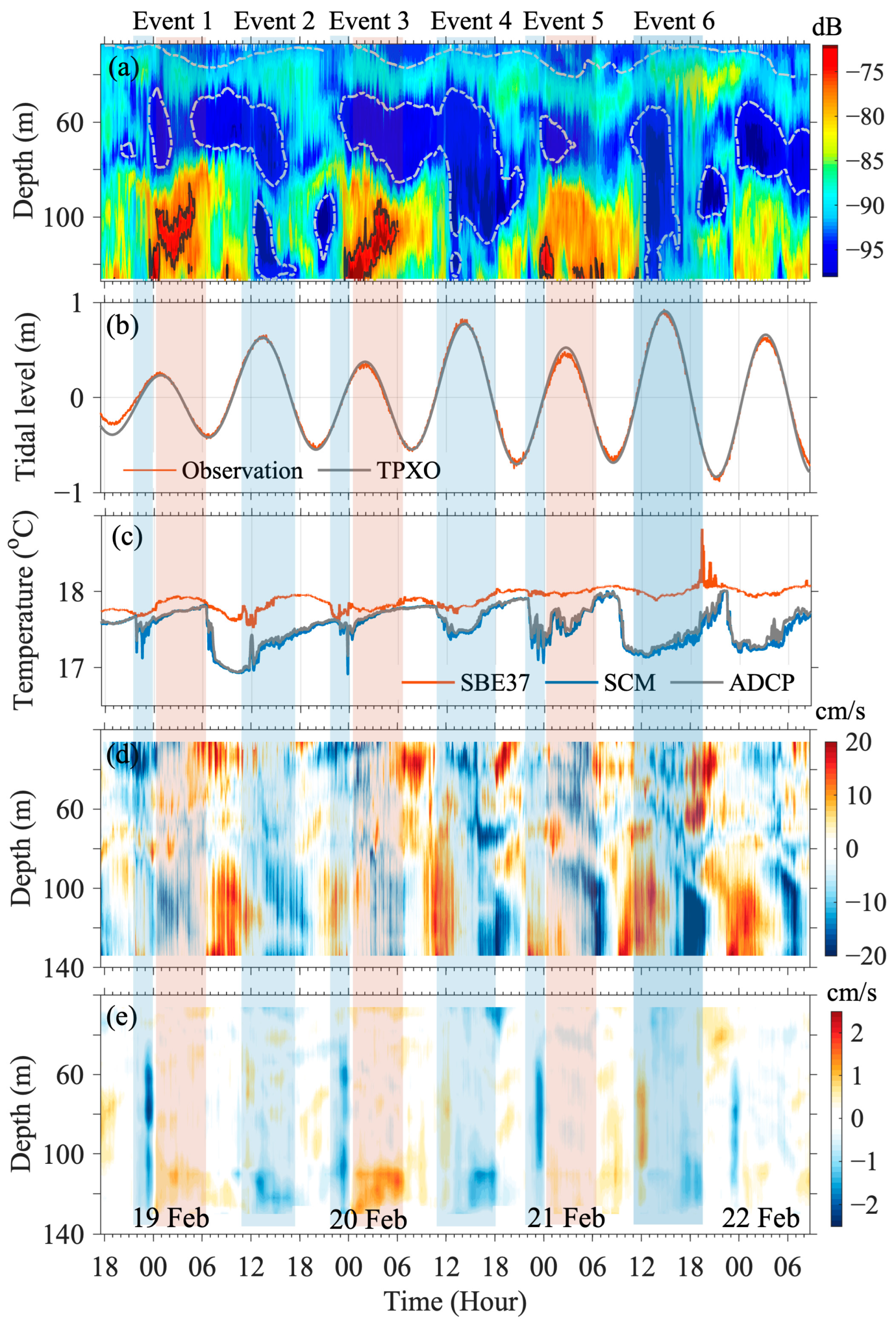
3.1. Variations of MVBS and Hydrological Condition

Figure 2a presents the distribution of hourly daily averaged variations in the MVBS, which is an indicator of suspended matters concentrations. Lower absolute values of MVBS indicate higher concentrations of suspended matters. Overall, both MVBSs from ADCP and turbidity from the CTD profiles at the mooring station revealed a three-layer structure in the distribution of suspended matters. In Figure 2b, two high-value regions are observed in the upper layer (depth above 50 m) and the lower layer (depth below 80 m), with a low-value region in the middle layer (depths between 50 and 80 m). The daily averaged variations in MVBS in the upper layer showed that the upper boundary of the high-value region descended to a depth below the surface of 30 m after sunrise and returned to the sea surface after sunset. The high-value region of MVBS in the lower layer concentrated below 80 m from 00:00 to 12:00 (UTC), reaching its maximum strength between 00:00 and 06:00. Simultaneously, the distribution of the MVBS revealed an interesting phenomenon: the high-value region in the lower layer completely disappeared between 12:00 and 18:00, with values approaching those of the low-value region in the middle layer.
During the observational period, the occurrence of hypoxia was captured by both of the CTD casts (Figure 2b). Figure 2c shows that dissolved oxygen decreases rapidly from a depth of 20 m and reaches 2 mg/L at a depth of 42 m (52 m) before deployment (after recovery) of the mooring. Observations of both the CTD casts showed significant changes in temperature and salinity above 80 m, indicating strong stratification above this depth. It is worth mentioning that in the second CTD cast, high-salinity, low-temperature, and low-turbidity seawater appeared near the seabed (approximately 140 m).
The two CTD casts at the mooring station were conducted at 16:35 (local nighttime) and 10:08 (local daytime) respectively. The turbidity near the sea surface during the nighttime (cast1) was significantly different than the observation during the daytime (cast2). Based on the continuous MVBS and the two profiles of turbidity observations, diel vertical migration was evident in the upper ocean. However, during the period of sunrise and sunset, the vertical migration was limited to depths above 60 m. In comparison with previous observations in the South China Sea [3] and the AS [4], the vertical migration depth range in our observation was smaller. During the daytime, the lower boundary of the high-value region of MVBS in the upper layer located in the depths above 60 m, which was close to the depth of the upper boundary of hypoxia.
In contrast to the relatively regular diurnal variations observed in the upper layer, the temporal changes in the MVBS in the lower layer exhibited greater complexity (Figure 3a). Throughout the observation period, three significant enhancements and three significant attenuations were recorded in the lower layer (Figure 3a). All three enhancement events took place between 00:00 and 06:00 each day (Events 1, 3, and 5), while the three attenuation events occurred between 12:00 and 18:00 each day (Events 2, 4, and 6). During the three enhancement events, the MVBS initially experienced a short-term decrease lasting approximately 2 h, followed by a significant increase. The impact depth reached a maximum of 80 m, and the duration of significant increase was 6 h. Figure 3b illustrates that the tidal cycle is irregular semidiurnal at the mooring station. Although both types of events occurred during the transition from high tide to low tide, the enhancement events took place during periods of small tidal amplitude, while the attenuation events occurred during periods of larger tidal amplitude.
Figure 3c presents the temporal distribution of temperature near the seabed. The temperature variation at a depth of 113 m (40 m above the seabed) was relatively small, while the temperature variation at a depth of 134 m (9 m above the seabed) was more pronounced, with a maximum daily temperature change exceeding 0.8 °C. In Figure 3c, the near-seabed temperature exhibits a spike-like signal, characterized by a sharp decrease between 21:00 and 23:00 daily. The horizontal current velocities were decomposed into along-slope and cross-slope components. The velocity in the along-slope direction was found to be stronger compared to the cross-slope direction, and it was dominated by semidiurnal cycle motions. Additionally, Figure 3d demonstrates that the variations in along-slope velocity also exhibit spike-like signals between 21:00 and 23:00 daily near the seabed, with a significant short-term increase. Similar processes, referred to as internal bores, have been observed in shallow water regions by the authors of [1,7]. The observed near-seabed variations in temperature and velocities occurring between 21:00 and 23:00 daily were likely attributed to the process of internal bores.
Figure 3d,e presents the depth–time distribution of horizontal and vertical current velocities. Horizontally, the velocity gradually increased and reached its maximum on 21 February, exceeding 20 cm/s (Figure 3d). The horizontal current exhibited a semidiurnal tidal cycle, with enhanced currents near the seabed. Additionally, within the depth range of 80 to 100 m, the onshore velocity observed before 00:00 was weaker and of shorter duration compared to the onshore velocities observed before 12:00. Vertically, a pair of negative–positive (positive–negative) velocities was observed around 00:00 (12:00) daily (Figure 3e). When the lower layers experienced short-term positive horizontal velocities, the vertical velocities initially showed short-term negative values (lasting no more than 2 h), followed by positive values lasting about 6 h. Conversely, when the lower layers experienced prolonged and significant positive horizontal velocities, the vertical velocities initially exhibited short-term positive values, followed by approximately 6 h of negative values. By examining the events of enhanced and reduced suspended matters, we found that the rapid increase in and diffusion of suspended matters from the seabed to a depth of 80 m corresponded to the vertical upward velocities, while the decrease in suspended matters in the lower layers corresponded to the vertical downward velocities.

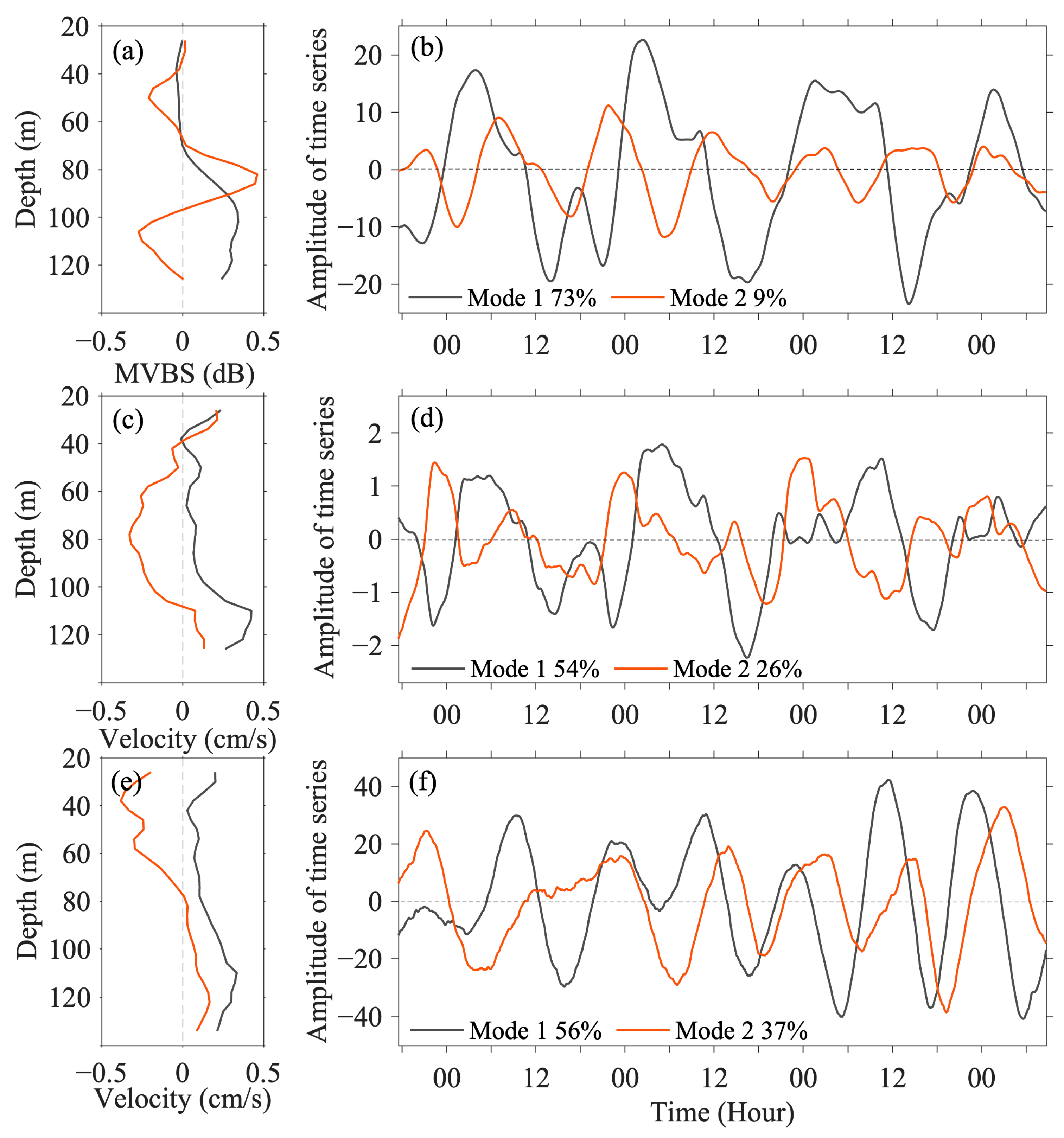
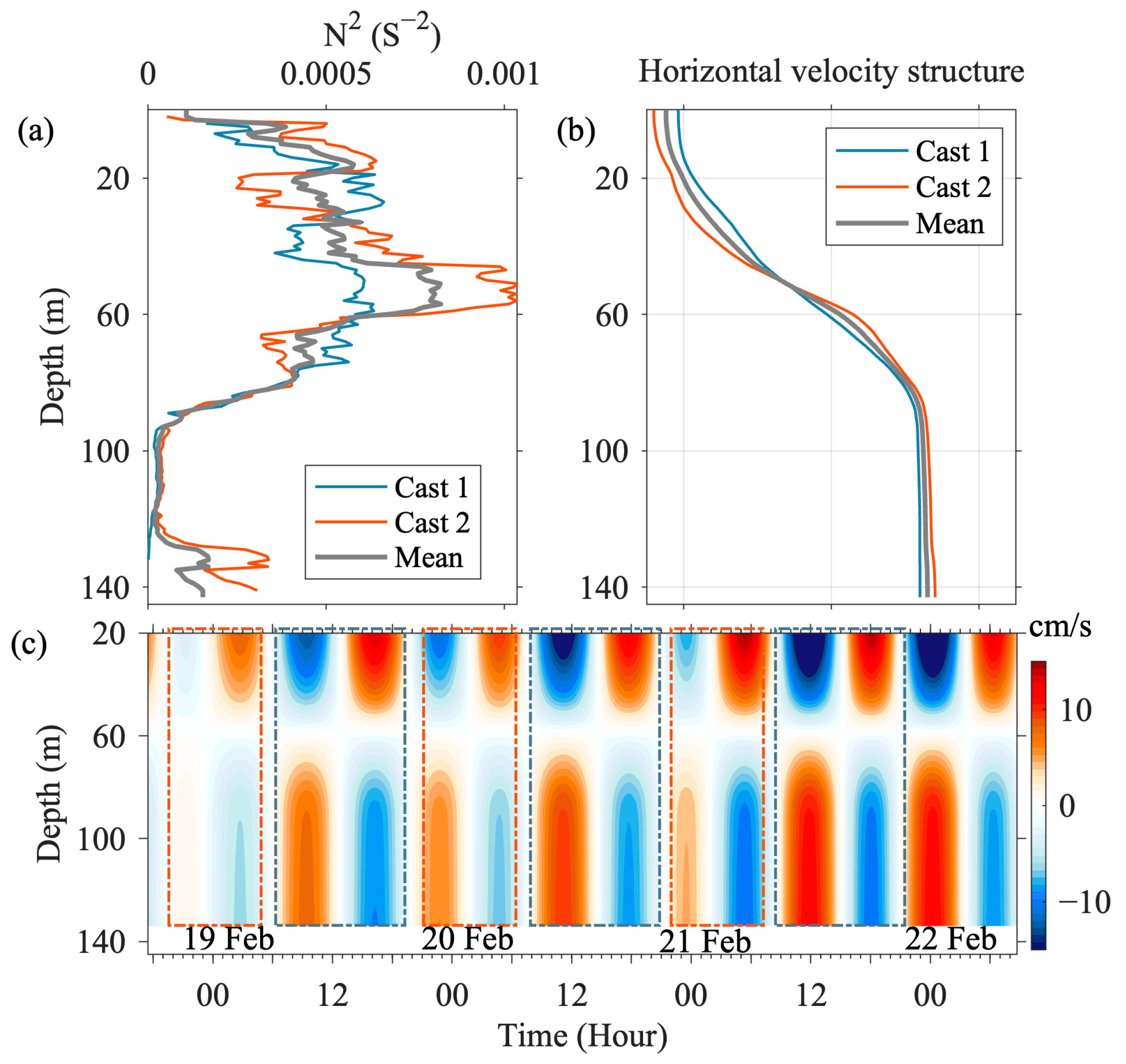
3.2. Modal Structure of MVBS and Currents in EOF and Semidriunal Internal Tides

To further investigate the temporal and spatial variations of MVBS and current velocities, an Empirical Orthogonal Function (EOF) decomposition was conducted on the MVBS, vertical, and horizontal velocities (Figure 4). Figure 4a,b presents the vertical distribution and time series of the two dominated modes of MVBS, respectively. The two modes account for 73% and 9% of the total variance, respectively. In Figure 4a, the first mode is nearly zero above 70 m but significantly increases below 80 m, primarily reflecting the change in MVBS in the low layers. The time series of the first mode exhibited a complex variation with signals at both diurnal and semidiurnal periods (Figure 4b). The second mode showed peaks at depths of 50, 82, and 106 m, with time series primarily displaying a semidiurnal period. The first two modes of vertical velocity accounted for 54% and 26% of the total variance (Figure 4c,d). In Figure 4c, the first mode exhibits high values below 100 m, closely resembling the distribution structure of MVBS’s first mode. Moreover, the correlation coefficient between the time coefficients of MVBS and vertical velocity, both for their first modes, reached 0.72. This suggested that MVBS below 100 m was predominantly influenced by vertical velocity. The spatial distributions of the first two modes in the horizontal velocity, which collectively explain 93% of the total variance, are shown in Figure 4e. The first mode, accounting for 56% of the variance, consistently exhibited a current direction throughout all depths. The second mode, contributing 37% of the variance, displayed a node at approximately 80 m, with opposing current directions between the upper and lower layers. The time series of both the first and second modes exhibited a semidiurnal tidal cycle, consistent with the local tidal characteristics mentioned earlier (Figure 4f). The time series of the first mode demonstrated a significant enhancement over time. The contributions of higher modes, which account for less than 10% of the variance, are not presented in this study.
In the horizontal velocity, the second mode of EOF analysis exhibited a zero node at a depth of 80 m, which resembled the vertical structure of the first dynamic mode of semidiurnal internal tides. To establish the correlation between the second EOF mode and the first dynamic mode, we utilized numerical methods to solve equations (Equations (7) and (8)). The buoyancy frequency in the equations was derived from the two casts of CTD (Figure 5a). As shown in Figure 5b, the zero node of the first dynamic mode of internal tides is located at a depth of 62 m. This indicates that the structure of the second EOF mode is primarily associated with the first baroclinic mode of internal tides. In contrast to the statistical decomposition of the EOF, we projected horizontal current velocity onto the dynamic modes. Figure 5c presents the depth–time variation of horizontal current velocities in the first dynamic mode of internal tides. Higher dynamical modes were relatively weak. The first-mode internal tides exhibited a maximum velocity amplitude of up to 12 cm/s. Moreover, it was observed that the first mode of semidiurnal internal tides also displayed variations similar to those of an irregular semidiurnal tide, with a weaker current around 00:00 and stronger current around 12:00 each day.
The vertical transport of suspended matters also could be significantly influenced by the mixing induced by shear instability [26,27]. Shear instability may occur when the Richardson number ( R i = N 2 / ( u / z 2 + v / z 2 )) is less than 0.25 [44,45]. Figure 6a presents the distribution of horizontal velocity shear and shows that the maximum shear occurs above 80 m and reaches 0.035 s−1. Significant temperature changes were observed at depths below 120 m based on CTD profiles and temperature observations in the mooring. The stratification below 120 m cannot be accurately represented by the averaged CTD profiles. Hence, the Ri was only calculated above 120 m and regions with Ri < 0.25 were highlighted using dashed lines. Although the maximum shear occurred above 80 m, the buoyancy frequency also reached its maximum around a depth of 80 m. Shear instability was only observed below a depth of 80 m (Figure 6a).
Figure 6b displays the depth-averaged Ri within the range of 90 to 118 m. The Ri values indicated the absence of shear instability between 00:00 and 06:00 daily. Notably, during the periods of 19 and 20 February, when suspended matters experienced a substantial increase, no occurrence of shear instability was observed within the same time frame. Therefore, the rise in suspended matters above depth of 120 m during enhanced events should not be attributed to mixing induced by the shear instability.

3.3. Qualitatively Estimation of Suspended Matters Transport

Due to the lack of calibration of the MVBS for suspended matters concentration, it was not possible to quantitatively calculate the flux of suspended matter. Instead, we estimated the qualitative flux of suspended matter by normalizing the MVBS. The normalized MVBS (NMVBS) was determined using the following formula: NMVBS = (MVBS − Min (MVBS))/(max (MVBS − min(MVBS))). The horizontal suspended matters flux due to advection was calculated using the normalized MVBS and horizontal velocities (Figure 7a). As shown in Figure 7b, there is a phase difference between the depth-averaged velocity and NMVBS. When NMVBS was relatively small, the increase in horizontal velocity did not result in significant changes in the strength of horizontal transport flux. However, when NMVBS was larger, the variation in horizontal flux exhibited a semidiurnal cycle (Figure 7c). Therefore, the temporal variation in horizontal transport flux was found to be complex, influenced by different phases of suspended matters and currents. In Figure 7d, the time-averaged horizontal transport flux over the entire observation period (spanning more than seven semidiurnal cycles) is presented. Throughout the observation period, the average suspended matter transport was offshore, with the strongest transport occurring at depths below 85 m.

4. Discussion

4.1. Suspended Matters in the Upper and Middle Layers

Previous studies have shown that the diel variations in the backscatter intensity of the ADCP are attributed to vertical migration of planktonic organisms [3,4,46,47]. The vertical migration of marine organisms is primarily triggered by the alternating light intensity between day and night. The authors of [4] have proposed that oxygen concentration might be the important factor influencing seasonal variations in the depths of the scattering layer in the AS. Relevant studies have indicated that most euphausiids and calanoid copepods tend to avoid areas with low oxygen [19], which happen to be the primary taxa within the AS ecosystem [48,49]. Additionally, the presence of hypoxia can constrain the distribution of aerobic predators [50]. Some migratory organisms descend to the upper boundary of the hypoxic region to evade aerobic predators [8]. For example, siphonophore and eucalanoid copepods are widespread within the AS [49] and have the habit of migration to the upper hypoxic region during daytime [19]. During the observation period, a hypoxic region was observed below a depth of 40 m (Figure 2b). It is hypothesized that organisms departed from the sea surface during daytime, with their downward movement being confined to the upper boundary of the hypoxic region. Consequently, the formation of a middle layer with low concentrations of suspended matter during the daytime is largely due to the presence of hypoxia. We consider that it is also the reason for the notably shallower vertical migration depths in our observation compared to other studies [3,4].
There was an increase in suspended matters in the middle layer (depth of 50–80 m) during the nighttime period from 18:00 to 00:00 (Figure 2a and Figure 3a), which was closely associated with the occurrence of enhanced semidiurnal internal tides (indicated by the blue box in Figure 5c). Theoretically, strong internal tides should result in larger fluctuations in the thermocline. The larger fluctuations induced by the stronger internal tides may contribute to the enhancement of the suspended matters in the middle layer. As the semidiurnal internal tides gradually intensified from 19 to 21 February, the middle-layer MVBS also showed enhancement during 18:00 to 00:00 (Figure 3a and Figure 6c). Particularly during 18:00 to 00:00 of 21 February, the MVBS in the middle layer reached its peak. At the same time, the temperature at a depth of 113 m increased sharply by 0.9 °C (Figure 3b), indicating downward movement of warm water in the upper layer. Both the distribution of the MVBS and temperature had a spike-like pattern, in accordance with the characteristics of internal solitary waves [51]. In terms of vertical transport depth, internal solitary waves exhibit greater strength compared to internal tides. We propose that internal solitary waves evolved from nonlinear steepening of semidiurnal internal tides when the internal tides were stronger. Unfortunately, due to the lack of temperature in the upper layer, the thermocline fluctuations induced by internal tides and internal solitary waves remain beyond the scope of our current investigation.

4.2. Suspended Matters in the Lower Layer

As previously mentioned, both the middle and lower layers were located within the hypoxic zone, where the variations in suspended matters showed limited correlation with sunrise and sunset (Figure 2a and Figure 3a). By examining the corresponding times of vertical velocity in relation to suspended matters (Figure 3a,e), analysis of EOF (Figure 4b,d), and previous studies [29,30], it can be concluded that the intensification (attenuation) of suspended matter primarily results from the uplift in (suppression of) vertical velocities. Additionally, it could be determined that the enhancement process from 80 to 120 m was unrelated to mixing caused by shear instability (Figure 6). In the analysis of EOF, both vertical and horizontal velocities exhibited shear in the vertical direction, presenting a baroclinic structure with tidal periodicity. Hence, both vertical and horizontal velocities are expected to be influenced by internal tides. But, why did the vertical velocity include signals with both diurnal and semidiurnal periods? Or, why did two pairs of completely different sequences of vertical velocities occur daily? As mentioned earlier, the local internal tides are dominated by the semidiurnal internal tides with an approximated 12 h period. In linear internal tides, horizontal velocities are typically an order of magnitude larger than vertical velocities. However, during the nonlinear evolution of internal tides, vertical velocities can significantly increase, reaching magnitudes comparable to horizontal velocities [51]. Therefore, the first mode in the EOF primarily reflected the vertical velocities excited during the nonlinear evolution of internal tides. When concerning horizontal velocity, it became evident that the first-order baroclinic mode dominated the characteristics of local semidiurnal internal tides (Figure 4f and Figure 5c). Weak (strong) semidiurnal internal tides corresponded to negative–positive (positive–negative) vertical velocities within the same day (Figure 3e and Figure 5c). During the shoaling of internal tides across the continental slope, internal bores could be generated from the internal tides [52]. Based on the sequences of appearance of vertical velocities, two types of internal bores can be distinguished. The first type consists of a pair of upward and downward vertical velocities appearing successively [53], while the second type consists of a pair of downward and upward vertical velocities appearing successively [23]. The formation of both types of internal bores is influenced by factors such as stratification, strength of internal tides, topographic slope, and so on [54,55]. Our observations indicated that the generation of the first (second) type occurred during periods of stronger (weaker) semidiurnal internal tides, which was similar to results from previous numerical simulation experiments [52]. The authors of [52] employed first-order baroclinic mode internal tides to drive their numerical model and generate the two types of internal bores by changing the intensity of internal tides. We considered that the varying intensities of semidiurnal internal tides might be responsible for the generation of different types of internal bores, resulting in two distinct patterns of vertical velocities.
Internal bores have been found to induce highly localized mixing [1]. In this study, the occurrence of shear instability was observed at a depth below 80 m (Figure 7a). The weak stratification observed below this depth was identified as the main factor contributing to the shear instability. Conversely, the pronounced stratification observed above 80 m prevented the onset of shear instability. In other words, the strong stratification above 80 m restricted the exchange of water masses between the middle and lower layer, making it difficult for suspended matters to be transported from the lower layers to the middle layers. As a result, a distinct boundary for suspended matter was observed at a depth of 80 m during the daytime (Figure 2a and Figure 3a). Additionally, due to the minimal temperature gradient below 80 m, the vertical velocity’s contribution to near-seabed temperature variation remained minimal. For instance, despite the downward velocity observed from 21:00 to 23:00 on 28 February (Figure 3a), a cooling process was observed (Figure 3c). Taking into account the strong onshore horizontal current near the seabed at the same time (Figure 3d), it was likely that the cooling process near the seabed originated from the horizontal onshore transport of deep water on the continental slope.

5. Conclusions

Though limited, the in situ data from CTD and mooring provided valuable insights into the profiles of temperature, salinity, turbidity, and oxygen, as well as time series data on temperature, currents, and acoustic backscatter for the continental shelf of the northern AS. This region is unique as it experiences both hypoxia and internal tides. The observations revealed that suspended matters exhibited a three-layer vertical structure with a low-value zone in the middle layer (50–80 m). The relationship between hydrodynamic conditions and suspended matters suggested that both oxygen concentration and internal tides played a role in influencing the variations observed in suspended matters.
In the upper layer (above 50 m), the upper boundary of the high-value region descended to a depth below the surface of 30 m after sunrise and returned to the surface after sunset, indicating a diel vertical migration of zooplankton and micronekton in the upper layer. During the period of sunrise and sunset, the vertical migration was limited to depths above 60 m. Our observation showed a smaller vertical migration depth range compared to previous observations in the South China Sea [3] and the AS [4]. The lower boundary of the high-value region in the upper layer was located at the depths above 60 m during the daytime, which was close to the depth of the upper boundary of hypoxia. We believed that the formation of the middle layer with low suspended matter concentrations during the daytime could be largely attributed to the presence of hypoxia, which explained the notably shallower vertical migration depths observed in our study compared to other studies.
In the lower layer (80–140 m), we observed three notable enhancements and three significant attenuations. The enhancements occurred daily between 00:00 and 06:00, while the attenuations occurred between 12:00 and 18:00. During the enhancement events, the MVBS experienced a temporary decrease lasting approximately 2 h, followed by a substantial increase. The impact depth reached 80 m and the duration of the enhancement events was 6 h. Additionally, we found a strong correlation between the enhanced (decreased) events and vertical upward (downward) velocities. The results of EOF suggested that MVBS below 100 m was predominantly influenced by vertical velocity.
We believed that the intensification (attenuation) of the suspended matters primarily results from the uplift in (suppression of) vertical velocities. It could be determined that the enhancement process from 80 to 120 m was unrelated to mixing caused by shear instability. Furthermore, the strong stratification above 80 m restricted the exchange of water masses between the middle and lower layer, making it difficult for suspended matter to be transported from the lower layers to the middle layers. Our findings indicate that the local semidiurnal internal tides are dominated by the first-order baroclinic mode. Weak (strong) semidiurnal internal tides corresponded to negative–positive (positive-negative) vertical velocities within the same day. We preliminarily speculated that the pattern of the vertical velocities was induced by the internal bores, which should be driven by the shoaling semidiurnal internal tides.

Author Contributions

Conceptualization, F.L., C.L. (Chujin Liang) and T.D.; methodology, F.L., D.Z. and C.Y.; formal analysis, F.L., X.M. and W.J.; writing—original draft preparation, F.L.; writing—review and editing, F.L., F.Z., H.L., B.Z. and C.L. (Chenggang Liu); supervision, F.L. and C.L. (Chujin Liang); funding acquisition, F.Z. All authors have read and agreed to the published version of the manuscript.

Funding

This research was funded by the Global Change and Air–Sea Interaction II project (grant Nos. GASI-01-EIND-STwin and GASI-04-WLHY-030) and the Joint Funds of the Zhejiang Provincial Natural Science Foundation of China (grant Nos. LQY20D060001).

Informed Consent Statement

Not applicable.

Data Availability Statement

The mooring data analyzed in this study are available on request from the corresponding author.

Acknowledgments

The authors thank the crew of R/V Xiangyanghong 06 for their considerable assistance in the cruise observation.

Conflicts of Interest

The authors declare no conflict of interest.

References

  1. Masunaga, E.; Homma, H.; Yamazaki, H.; Fringer, O.B.; Nagai, T.; Kitade, Y.; Okayasu, A. Mixing and sediment resuspension associated with internal bores in a shallow bay. Cont. Shelf Res. 2015, 110, 85–99. [Google Scholar]
  2. Tian, Z.; Jia, Y.; Chen, J.; Liu, J.P.; Zhang, S.; Ji, C.; Liu, X.; Shan, H.; Shi, X.; Tian, J. Bottom and intermediate nepheloid layer induced by shoaling internal solitary waves: Impacts of the angle of the wave group velocity vector and slope gradients. J. Geophys. Res. Oceans 2019, 124, 5686–5699. [Google Scholar]
  3. Yang, C.; Xu, D.; Chen, Z.; Wang, J.; Xu, M.; Yuan, Y. Diel vertical migration of zooplankton and micronekton on the northern slope of the South China Sea observed by a moored ADCP. Deep-Sea Res. Part II 2019, 167, 93–104. [Google Scholar]
  4. Liu, Y.; Guo, J.; Xue, Y.; Sangmanee, C.; Wang, H.; Zhao, C.; Khokiattiwong, S.; Yu, W. Seasonal variation in diel vertical migration of zooplankton and micronekton in the Andaman Sea observed by a moored ADCP. Deep-Sea Res. Part I 2022, 179, 103663. [Google Scholar]
  5. Oliveira, A.; Vitorino, J.; Rodrigues, A.; Jouanneau, J.M.; Dias, J.A.; Weber, O. Nepheloid layer dynamics in the northern Portuguese shelf. Prog Oceanogr. 2002, 52, 195–213. [Google Scholar]
  6. Inthorn, M.; Mohrholz, V.; Zabel, M. Nepheloid layer distribution in the Benguela upwelling area offshore Namibia. Deep-Sea Res. Part I 2006, 53, 1423–1438. [Google Scholar]
  7. Masunaga, E.; Arther, R.S.; Fringer, O.B.; Yamazaki, H. Sediment resuspension and the generation of intermediate nepheloid layers by shoaling internal bores. J. Mar. Syst. 2017, 170, 31–41. [Google Scholar]
  8. Bianchi, D.; Galbraith, E.D.; Carozza, D.A.; Mislan, K.A.S.; Stock, C.A. Intensification of open-ocean oxygen depletion by vertically migrating animals. Nat. Geosci. 2013, 6, 545–548. [Google Scholar]
  9. Jia, Y.; Tian, Z.; Shi, X.; Liu, J.P.; Chen, J.; Liu, X.; Ye, R.; Ren, Z.; Tian, J. Deep-sea Sediment Resuspension by Internal Solitary Waves in the Northern South China Sea. Sci. Rep. 2019, 9, 12137. [Google Scholar]
  10. Bruland, K.W.; Rue, E.L.; Smith, G.J. Iron and macronutrients in California coastal upwelling regimes: Implications for diatom blooms. Limnol. Oceanogr. 2001, 46, 1661–1674. [Google Scholar]
  11. Wang, Z.; DiMarco, S.F.; Ingle, S.; Belabbassi, L.; AI-Kharusi, L.H. Seasonal and annual variability of vertically migrating scattering layers in the northern Arabian Sea. Deep-Sea Res. Part I. 2014, 90, 152–165. [Google Scholar]
  12. Wang, H.; Chen, H.; Xue, L.; Liu, N.; Liu, Y. Zooplankton diel vertical migration and influence of upwelling on the biomass in the Chukchi Sea during summer. Acta Oceanol. Sin. 2015, 34, 68–74. [Google Scholar]
  13. Haney, J.F. Diel patterns of zooplankton behaviors. Bull. Mar. Sci. 1988, 43, 583–603. [Google Scholar]
  14. Cohen, J.H.; Forward, R.B. Spectral sensitivity of vertically migrating marine copepods. Biol. Bull. 2002, 203, 307–314. [Google Scholar] [PubMed]
  15. Wishner, K.F.; Outram, D.M.; Seibel, B.A.; Daly, K.L.; Williams, R.L. Zooplankton in the eastern tropical north Pacific: Boundary effects of oxygen minimum zone expansion. Deep-Sea Res. Part I 2014, 90, 152–165. [Google Scholar]
  16. Rabouille, C.; Conley, D.J.; Dai, M.H.; Cai, W.J.; Chen, C.T.A.; Lansard, B.; McKee, B. Comparison of hypoxia among four river-dominated ocean margins: The Changjiang (Yangtze), Mississippi, Pearl, and Rhone rivers. Cont. Shelf Res. 2008, 28, 1527–1537. [Google Scholar]
  17. Zhou, F.; Huang, D.; Ni, X.; Xuan, J.; Zhang, J.; Zhu, K. Hydrographic analysis on the multi-time scale variability of hypoxia adjacent to the Changjiang River Estuary. Acta Oceanol. Sin. 2010, 17, 4728–4740, (In Chinese with English Abstract). [Google Scholar]
  18. Cade, D.E.; Benoit-Bird, K.J. Depths, migration rates and environmental associations of acoustic scattering layers in the Gulf of California. Deep-Sea Res. Part I 2015, 102, 78–89. [Google Scholar]
  19. Hauss, H.; Christiansen, S.; Schütte, F.; Kiko, R.; Lima, M.E.; Rodrigues, E.; Karstensen, J.; Löscher, C.R.; Körtzinger, A.; Fiedler, B. Dead zone or oasis in the open ocean? Zooplankton distribution and migration in low-oxygen modewater eddies. Biogeosciences 2016, 13, 1977–1989. [Google Scholar]
  20. Garrett, C.; Kunze, E. Internal Tide Generation in the Deep Ocean. Annu. Rev. Fluid Mech. 2007, 39, 57–87. [Google Scholar]
  21. Ma, X.; Yan, J.; Hou, Y.; Lin, F.; Zheng, X. Footprints of obliquely incident internal solitary waves and internal tides near the shelf break in the northern South China Sea. J. Geophys. Res. Oceans 2016, 121, 8706–8719. [Google Scholar]
  22. Quaresma, L.S.; Vitorino, J.; Oliveira, A.; Silva, J. Evidence of sediment resuspension by nonlinear internal waves on the western Portuguese mid-shelf. Mar. Geol. 2007, 246, 123–143. [Google Scholar]
  23. Klymak, J.M.; Moum, J.N. Internal solitary waves of elevation advancing on a shoaling shelf. Geophys. Res. Lett. 2003, 30, 2045. [Google Scholar]
  24. Bogucki, D.; Dickey, T.; Redekopp, L.G. Sediment Resuspension and Mixing by Resonantly Generated Internal Solitary Waves. J. Phys. Oceanogr. 1997, 27, 1181–1196. [Google Scholar]
  25. Aghsaee, P.; Boegman, L. Experimental investigation of sediment resuspension beneath internal solitary waves of depression. J. Geophys. Res. Oceans 2015, 120, 3301–3314. [Google Scholar]
  26. Cacchione, D.; Wunsch, C. Experimental study of internal waves over a slope. J. Fluid Mech. 1974, 66, 223–239. [Google Scholar]
  27. Helfrich, K.R. Internal solitary wave breaking and run-up on a uniform slope. J. Fluid Mech. 1992, 243, 133–154. [Google Scholar]
  28. Cacchione, D.A.; Drake, D.E. Nepheloid layers and internal waves over continental shelves and slopes. Geo-Marine Lett. 1986, 6, 147–152. [Google Scholar]
  29. Lamb, K.G. Particle transport by nonbreaking, solitary internal waves. J. Geophys. Res. Oceans 1997, 102, 18641–18660. [Google Scholar]
  30. Ribbe, J.; Holloway, P.E. A model of suspended sediment transport by internal tides. Cont. Shelf Res. 2001, 21, 395–422. [Google Scholar]
  31. Sridevi, B.; Sarma, V.V. A revisit to the regulation of oxygen minimum zone in the Bay of Bengal. J. Earth Syst. Sci. 2020, 129, 107. [Google Scholar]
  32. Baronas, J.J.; Stevenson, E.I.; Hackney, C.R.; Darby, S.E.; Bickle, M.J.; Hilton, R.G.; Larkin, C.S.; Parsons, D.R.; Khaing, A.M.; Tipper, E.T. Integrating Suspended Sediment Flux in Large Alluvial River Channels: Application of a Synoptic Rouse-Based Model to the Irrawaddy and Salween Rivers. J. Geophys. Res. Earth Surf. 2020, 125, e2020JF005554. [Google Scholar]
  33. Osborne, A.; Burch, T. Internal solitions in the Andaman Sea. Science 1980, 208, 451–460. [Google Scholar]
  34. Alper, W.; Heng, W.C.; Lim, H. Observation of internal waves in the Andaman Sea by ERS SAR. In Proceedings of the IGARSS’97. 1997 IEEE International Geoscience and Remote Sensing Symposium Proceedings. Remote Sensing-A Scientific Vision for Sustainable Development, Singapore, 3–8 August 1997; pp. 1518–1520. [Google Scholar]
  35. Mohanty, S.; Rao, A.D.; Latha, G. Energetics of semidiurnal internal tides in the Andaman Sea. J. Geophys. Res. Oceans 2018, 123, 6224–6240. [Google Scholar]
  36. Magalhaes, J.M.; Da Silva, J.C.B. Internal Solitary Waves in the Andaman Sea: New Insights from SAR Imagery. Remote Sens. 2018, 10, 861. [Google Scholar]
  37. Jackson, C.; Silva, J.; Jeans, G. The generation of nonlinear internal waves. Oceanography. 2012, 25, 108–123. [Google Scholar]
  38. Cai, S.; Wu, Y.; Xu, J.; Chen, Z.; Xie, J.; He, Y. On the generation and propagation of internal solitary waves in the southern Andaman Sea: A numerical study. Sci. China Earth Sci. 2021, 64, 1674–1686. [Google Scholar]
  39. Yang, Y.; Huang, X.; Zhao, W.; Zhou, C.; Huang, S.; Zhang, Z.; Tian, J. Internal Solitary Waves in the Andaman Sea Revealed by Long-Term Mooring Observations. J. Phys. Oceanogr. 2021, 51, 3609–3627. [Google Scholar]
  40. Jithin, A.; Francis, P. Role of Internal Tide Mixing in Keeping the Deep Andaman Sea Warmer Than the Bay of Bengal. Sci. Rep. 2020, 10, 11982. [Google Scholar]
  41. Egbert, G.D.; Erofeeva, S.Y. Efficient inverse modeling of barotropic ocean tides. J. Atmos. Ocean. Technol. 2002, 19, 183–204. [Google Scholar]
  42. Deines, K.L. Backscatter estimation using broadband acoustic Doppler current profilers. In Proceedings of the IEEE Sixth Working Conference on Current Measurement, San Diego, CA, USA, 11–13 March 1999; pp. 249–253. [Google Scholar]
  43. Cao, A.; Guo, Z.; Pan, Y.; Song, J.; He, H.; Li, P. Near-Inertial Waves Induced by Typhoon Megi (2010) in the South China Sea. J. Mar. Sci. Eng. 2021, 9, 440. [Google Scholar]
  44. Kundu, P.K.; Beardsley, R.C. Evidence of a critical Richardson number in moored measurements during the upwelling season off northern California. J. Geophys. Res. 1991, 96, 4855–4868. [Google Scholar]
  45. Xu, J.; Xie, J.; Chen, Z.; Cai, S.; Long, X. Enhanced mixing induced by internal solitary waves in the South China Sea. Cont. Shelf Res. 2012, 49, 34–43. [Google Scholar]
  46. Lü, L.; Wang, X.; Wang, H.; Li, L.; Yang, G. The variations of zooplankton biomass and their migration associated with the Yellow Sea Warm Current. Cont. Shelf Res. 2013, 64, 10–19. [Google Scholar]
  47. Luo, J.; Ortner, P.B.; Forcucci, D.; Cummings, R.C. Diel vertical migration of zooplankton and mesopelagic fish in the Arabian Sea. Deep-Sea Res. Part II 2000, 47, 1451–1473. [Google Scholar]
  48. Goswami, S.C.; Rao, T.; Matondkar, S. Biochemical composition of zooplankton from the Andaman Sea. Indian J. Mar. Sci. 1981, 10, 296–300. [Google Scholar]
  49. Jitlang, I.; Pattarajinda, S.; Mishra, R. Composition, Abundance and Distribution of Zooplankton in the Bay of Bengal. Ecosyst. Based Fish. Manag. Bay Bengal 2008, 65–92. [Google Scholar]
  50. Seibel, B.A. Critical oxygen levels and metabolic suppression in oceanic oxygen minimum zones. J. Exp. Biol. 2011, 214, 326–336. [Google Scholar]
  51. Xu, A.; Chen, X. A Strong Internal Solitary Wave with Extreme Velocity Captured Northeast of Dong-Sha Atoll in the Northern South China Sea. J. Mar. Sci. Eng. 2021, 9, 1227. [Google Scholar]
  52. Dauhajre, D.P.; Molemaker, M.J.; Mcwilliams, J.C.; Hypolite, D. Effects of stratification on shoaling internal tidal bores. J. Phys. Oceanogr. 2021, 51, 3183–3202. [Google Scholar]
  53. McSweeney, J.M.; Lerczak, J.A.; Barth, J.A.; Becherer, J.; Colosi, J.A.; MacKinnon, J.A.; MacMahan, J.H.; Moum, J.N.; Pierce, S.D.; Waterhouse, A.F. Observations of shoaling nonlinear internal bores across the central California inner shelf. J. Phys. Oceanogr. 2020, 50, 111–132. [Google Scholar]
  54. Walter, R.K.; Woodson, C.B.; Leary, P.R.; Monismith, S.G. Connecting wind-driven upwelling and offshore stratification to nearshore internal bores and oxygen variability. J. Geophys. Res. Oceans 2014, 119, 3517–3534. [Google Scholar]
  55. Colosi, J.; Kumar, N.; Suanda, S.; Freismuth, T.; MacMahan, J. Statistics of internal tide bores and internal solitary waves observed on the inner continental shelf off of Point Sal, California. J. Phys. Oceanogr. 2018, 48, 123–143. [Google Scholar]
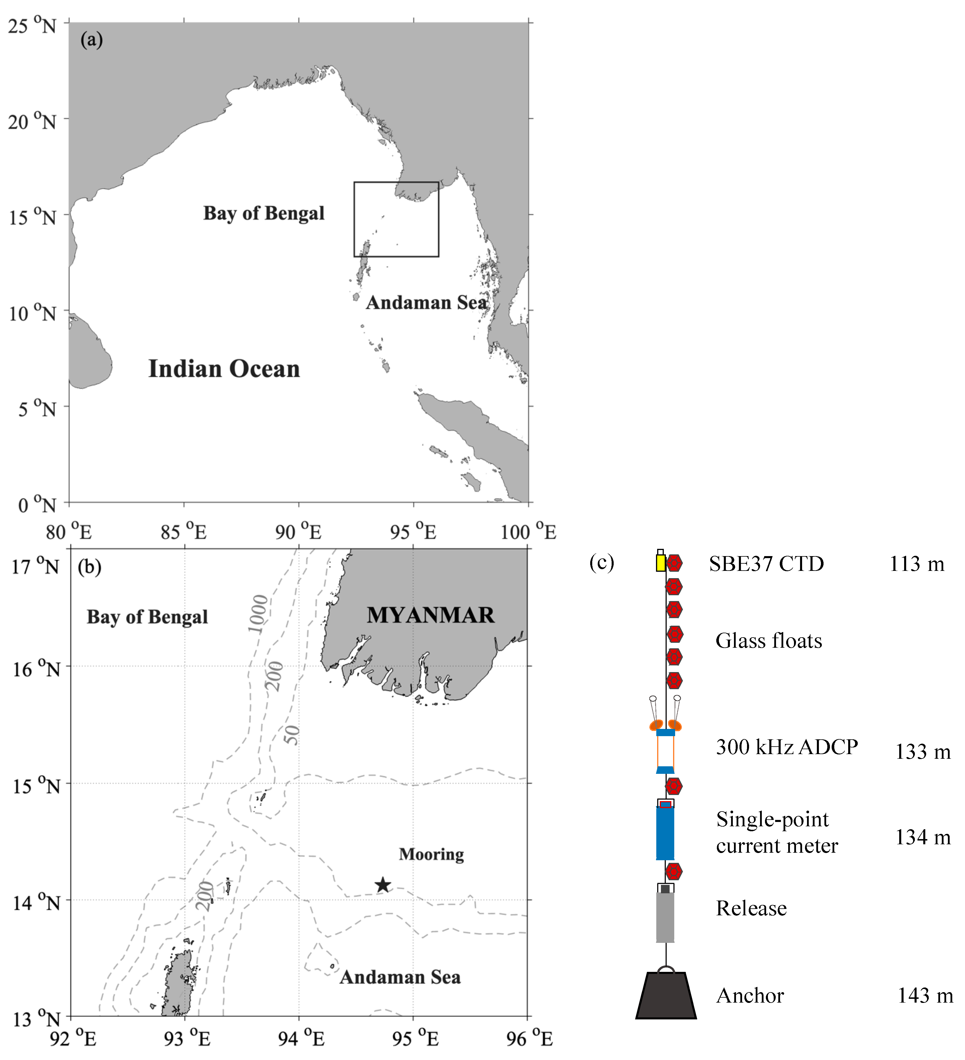
Figure 1. Study area and instrument locations: (a) Map of the northeastern Indian Ocean. (b) Zoom in of region highlighted in the black box of (a), bathymetry contours and locations of the mooring and CTD station (black star). (c) Schematic of mooring configuration. Refer to Table 1 for details of in situ stations.
Jmse 11 01950 g001
Figure 2. (a) Mean diurnal cycle of mean volume backscattering strength. The blue dash lines indicate the times of sunrise and sunset. The vertical profiles of turbidity (b), dissolved oxygen (c), temperature and salinity (d) from two casts at the mooring station before the mooring deployment (black line) and after recovery (gray line).
Jmse 11 01950 g002
Figure 3. Distribution: (a) MVBS; (b) Tidal elevation; (c) Temperature. Three temperature sensors, including SBE37, ADCP, and a single-point current meter (SCM), were used to observed the temperature at depths of 113 m (red), 133 m (gray), and 134 m (blue), respectively. (d) Depth–time plots of horizontal velocity in alone-slope direction. Positive values in the horizontal velocities represent onshore velocities. (e) Depth–time plots of vertical velocity.
Jmse 11 01950 g003
Figure 4. Vertical distribution of the two dominated modes (left panel) and their correspond time series (right panel) from EOF analysis of the following: (a,b) MVBS; (c,d) Vertical velocity; (e,f) Horizontal velocity. The dashed lines represent the position at zero.
Jmse 11 01950 g004
Figure 5. (a) Buoyancy frequency profiles of cast 1, cast 2, and the average of the two casts. (b) The first dynamic modes for the internal tide. (c) Depth–time plots of horizontal velocity induced by the mode-1 internal tides.
Jmse 11 01950 g005
Figure 6. (a) Depth–time plot of vertical shear of horizontal currents. The dashed lines represent the zones where the Richardson number was lower than 0.25. (b) Depth-averaged (90~118 m) Richardson number. The red (grey) lines indicate the value lower (larger) than 0.25.
Jmse 11 01950 g006
Figure 7. (a) Depth–time plots of flux of suspended matters. Positive (negative) values represent an onshore (offshore) transport (unit: 1× cm/s). (b) Depth-averaged (from 86 m to 124 m) suspended matters (blue) and along-slope velocity (red, unit: cm/s). (c) Transport of suspended matters. (d) Time-averaged flux of suspended matters during the observational period. The dashed line represents averaged flux variations in depths.
Jmse 11 01950 g007
Table 1. Information on in situ measurement.
MooringLocation
94.74° E, 14.12° N
Deployment Time
18–22 February (UTC)
InstrumentSampling information Variable
SBE 371 min at 113 mTemperature, salinity, and pressure
300 kHz
ADCP
3 min (27 × 4 m bins)
upward-looking at 133 m
Current and temperature
Single-point current meter3 min at 134 mCurrent, temperature, and pressure
CTDDeployment TimeVariable
Cast 1
Cast 2
16:35 18 February (UTC)
10:08 22 February (UTC)
Temperature, salinity, dissolved oxygen, and turbidity
Disclaimer/Publisher’s Note: The statements, opinions and data contained in all publications are solely those of the individual author(s) and contributor(s) and not of MDPI and/or the editor(s). MDPI and/or the editor(s) disclaim responsibility for any injury to people or property resulting from any ideas, methods, instructions or products referred to in the content.

