Model-Free Adaptive Sliding Mode Control Method for Unmanned Surface Vehicle Course Control

Abstract

A novel data-driven-based adaptive sliding-mode control scheme is proposed for unmanned surface vehicle course control in the presence of disturbances. The proposed method utilizes the model-free adaptive control (MFAC) theory. On account of the unknown dynamics of the USV course system, the control scheme is only established by online input and output information of the system. Based on a model-free adaptive control scheme, the system disturbance estimation technique is applied to compensate for the disturbances in the established compact form dynamic linearization data model. The controller is designed and combined with the sliding mode method, and a second-order switching surface with a fast terminal sliding function is employed to achieve finite-time convergence. Furthermore, an analysis of the stability of the control system is provided. Finally, MATLAB simulations are implemented to verify the validity and robustness of the proposed control scheme by comparing it with PID and typical model-free adaptive sliding mode control.

1. Introduction

An intelligent ship with autonomous functionalities, the Unmanned Surface Vehicle (USV) possesses the ability to undertake a range of tasks by incorporating diverse equipment modules. These tasks encompass surveys, search and rescue operations, salvage missions, waste recycling and more. Many scholars and engineers have conducted extensive research on the USV. The USV operates with a sophisticated control system due to its inherent traits of nonlinearity, uncertainty and dynamic variability. Developing a precise dynamic mathematical model for the USV proves to be a formidable challenge. As the USV navigates at varying speeds, substantial alterations occur in crucial physical parameters such as hull wetting area and draft, consequently inducing shifts in the hydrodynamic coefficients of the hull. Besides this, the large influence of environmental disturbances also affects the accuracy of the model. Due to the difficulty in describing time-varying disturbances using mathematical models, the control algorithm proposed by the conventional mathematical models lacks adaptability and ensuring the stability and robustness of the control system is a challenging task.

Course control for USVs is an essential and foundational issue. There are four main types of mathematical models for USV course control, such as Nomoto [1], Norribin [2,3], MMG [4] and Fossen [5]. Based on these mathematical models, many methods have been applied to solve the course control, achieving desirable theoretical results, mainly including PID control [6], ADRC [7], dynamic surface control [8,9], sliding mode control [10,11], intelligent control [12,13] and other methods. However, apart from PID, most of the other methods mentioned above have not been verified on actual USV. In actual physical systems, in addition to external disturbances and system parameter uncertainty, there are also problems such as time delay in the system [14]. These all increase the difficulty of control.

Apart from the conventional control methods mentioned above, to design a control law for data-driven methods, only input and output data are used instead of an accurate mathematical model of the controlled system. Therefore, the primary benefit of data-driven methods resides in their capacity to design controllers without the need for a precise mathematical model of the system. By learning from the actual system responses, data-driven techniques can effectively capture the system’s characteristics and provide control strategies that accommodate the inherent complexities and uncertainties often present in real-world systems.

According to the controller structure, these data-driven methods can be divided into two categories [15]. The methods with a known controller structure belong to the first category. The designer is tasked with identifying an appropriate controller structure. Examples of this category encompass methods such as virtual reference feedback tuning, iterative feedback tuning and unfalsified control. In the second category, the controller structure is not necessarily known. Subspace predictive control, iterative learning control and MFAC are representative types within this classification. Differing from the first class, the methods in this class have more robustness in an actual environment. Besides the advantages of an unknown controller structure, MFAC also has attractive properties. External testing and training process is not required, and the control approach is straightforward and readily implementable [15].

Hou et al. [16,17] have constructed and improved the theoretical framework and content of MFAC and have completed some research work. MFAC has found application in numerous nonlinear and complex systems, such as quadrotors [18], morphing vehicles [19], unmanned ground vehicles [20], autonomous underwater vehicles [21], absorption refrigeration systems [22], etc. MFAC also applies to USV control. For USV trajectory tracking, a novel control approach is formulated by combining PID control and sliding mode control techniques [23]. In [24], a new data-driven PI-type sliding-mode surface is proposed within backstepping. For USV path following, a data-driven sideslip observer-based line-of-sight guidance law is designed, and a data-driven SMC approach is developed for data-driven velocity controllers [25].

In [26], the indirect realization of the USV course control is achieved through the utilization of the angular velocity guidance algorithm within the outer loop. The CFDL-MFAC is applied for angular velocity control in the inner loop. To realize direct control of the heading angle, the redefined output CFDL-MFAC method is introduced by incorporating a redefined system-controlled output. The newly defined system output is obtained as the linear sum of the heading angle and angular velocity [27]. Drawing on the concept of redefined system output, the new output is the linear sum of the input and output information of the controlled system [28]. In order to address the control performance sensitivity of the system to the redefined output gain of RO-CFDL-MFAC, a controller output constraint function is proposed [29]. In order to tackle the challenges associated with overshooting, oscillations and sluggish convergence in the heading control using the MFAC approach, an adaptive forgetting factor is incorporated into the CFDL-MFAC method [30], and a variable integral separation model-free adaptive control algorithm is proposed with proportional control and variable integral separation factor [31].

While MFAC operates independently of the USV mathematical model, and time-varying parameter pseudo partial derivative (PPD), pseudo gradient (PG) or pseudo-Jacobian matrix (PJM) are updated online through the system I/O data by the estimation algorithm. This means a certain adaptive ability of MFAC to the disturbances. However, for a complex nonlinear system with disturbances, the estimation of PPD in the MFAC is not accurate enough. Hence, Ref. [32] demonstrates that when the system has disturbance, the performance of the control system based on MFAC will still be affected. In [33], the RBFNN-MFAC approach is introduced as a means of enhancing controller performance by integrating radial basis function neural networks to predict the value of PPD. In another approach [34], to obtain accurate PPD, the observer technique is adopted to tackle the issues of parametric perturbations and unknown external disturbances.

In addition, in the field of control, the distinctive attributes of robustness, rapid convergence rate and simplicity have led to substantial interest in sliding mode control. Therefore, in [32], model-free adaptive sliding mode control (MFASMC) is first developed. MFASMC still utilizes the model-free adaptive control algorithm framework, but SMC law is used instead of control law based on the optimal objective function. Specifically, the SMC method is used to calculate the control increment in the dynamic linearized data model. In [31], the MFASMC method is proposed for discrete-time single-input single-output (SISO) systems, and the reaching law is chosen as the exponential reaching law. Based on the MFASMC framework, many MFASMC methods have been developed. In [35], a multi-degree-of-freedom robotic exoskeleton employs an analogous reaching law to introduce the concept of MFASMC. In [36], a new MFASMC is designed with the terminal SMC technique for MIMO systems. In this work, in order to enhance the control system’s performance even further, the control scheme is proposed using the prescribed performance control method. Similar work is completed in complex industrial processes [37]. For the purpose of augmenting the control authority of MFASMC, a novel stabilizing sliding variable is introduced [38]. In [39], a high-order switching surface is used to design a model-free high-order TSMC law to mitigate the chattering problem.

Drawing upon the aforementioned research findings, the paper delves into the discussion of USV course control using the model-free adaptive sliding mode control method. The principal work of this paper includes:

• For the USV course control system with disturbance, a data-based model is established based on the nonparametric dynamic linearization technique. The disturbance estimation method is adopted to estimate unknown disturbance terms in the data-based model;
• A new approach to adaptive sliding mode control without relying on a model has been introduced, which uses second-order discrete sliding mode function and fast terminal sliding mode surface to attain quicker convergence rates and improved robustness compared to conventional SMC methods;
• The stability of the USV course control system under the proposed MFASMC method is proved. Simulation outcomes of the proposed approach are contrasted with those of PID control and model-free linear sliding mode control. Compared results show that the proposed MFASMC method has better tracking performance for the USV course control system in the presence of disturbances.

The subsequent sections of the paper are structured as follows: Section 2 elaborates on the dynamic linearization technique for the USV course control problem, along with some preliminary issues about the CFDL-MFAC. The design process of model-free second-order fast terminal sliding mode control is outlined in Section 3. Section 4 introduces the stability analysis of the closed-loop system governed by the proposed MFASMC approach. Comparative simulation results by different methods are illustrated in Section 5. Finally, the primary conclusions of the paper are summarized in Section 6.

2. Problem Formulation

Throughout the paper, $\left|·\right|$ denotes the absolute operator, $‖·‖$ is the Euclidean norm, and $\widehat{\left(·\right)}$ is the estimate of $\left(·\right)$. Therefore, the estimation error is represented by $\widetilde{\left(·\right)}=\widehat{\left(·\right)}-\left(·\right)$.

The course control system for USV can be expressed as

$$\left\{\begin{array}{l}\dot{\psi }=r,\\ \dot{r}=f\left(r,\delta \right)+d\left(t\right),\end{array}\right.$$

(1)

where $\psi$ is the course angle and $\psi \in \left[-{180}^{°},{180}^{°}\right]$. $r$ is the angular velocity. $d\left(t\right)$ is the time-varying bounded disturbance, which satisfies the condition $\left|d\left(t\right)\right|\le d_0$, $d_0>0$. $\delta$ is the rudder angle. Noting the saturation characteristics of the rudder angle, the maximum value of control input $\delta$ of the course control system is limited to $\delta \in \left[-{30}^{°},{30}^{°}\right]$. For the second equation of (1), the subsystem takes the rudder angle $\delta$ as its input and produces the angular velocity $r$ as its output. In addition, function $f\left(r,\delta \right)$ is unknown.

Within the MFAC methodology, three dynamic linearization control schemes exist: CFDL-MFAC, PFDL-MFAC and FFDL-MFAC. This paper delves into the USV course control issue by the CFDL-MFAC control scheme, taking into account the characteristics of the USV system. Meanwhile, the USV course system can be expressed as a SISO nonlinear discrete-time system

$$\psi (k+1)=f\left(\psi (k+1),\dots ,\psi \left(k-n_{\psi }\right),\delta (k),\dots ,\delta \left(k-n_{\delta }\right)\right)+d(k),$$

(2)

where $\psi \left(k+1\right)$ and $\delta \left(k\right)$ respectively represent the output of the system (1) at time $k+1$ and the input at time $k$. $n_{\psi }$ and $n_{\delta }$ are the orders of the system.

Let

$${\psi }_m\left(k+1\right)=f\left(\psi \left(k+1\right),\dots ,\psi \left(k-n_{\psi }\right),\delta \left(k\right),\dots ,\delta \left(k-n_{\delta }\right)\right)$$

(3)

From (2) and (3), we get

$$\psi \left(k+1\right)={\psi }_m\left(k+1\right)+d\left(k\right),$$

Therefore, it can be obtained that

$$∆\psi \left(k+1\right)=∆{\psi }_m\left(k+1\right)+∆d\left(k\right),$$

(4)

where $∆\psi \left(k+1\right)=\psi \left(k+1\right)-\psi \left(k\right)$, $∆{\psi }_m\left(k+1\right)={\psi }_m\left(k+1\right)-{\psi }_m\left(k\right)$ and $∆d\left(k\right)=d\left(k\right)-d\left(k-1\right)$.

The core idea behind the MFAC approach involves creating a dynamic linear data model that equals a nonlinear system at each operational state. Before introducing MFAC, the course control system described by (3) is assumed to satisfy the following assumptions [17]:

Assumption 1:

The input and output of the system (1) are measured and controllable, meaning that for any bounded desired output signal ${\psi }_d\left(k+1\right)$, it is always possible to find a bounded control input signal that results in the system’s output being equivalent to ${\psi }_d\left(k+1\right)$.

Assumption 2:

Except for finite moment, the partial derivatives of $f\left(\cdots \right)$ with respect to control input $\delta \left(k\right)$ are continuous.

Assumption 3:

With the exception of finite time moments, the system (1) meets the criteria of the generalized Lipschitz condition $\left|{\psi }_m\left(k_1+1\right)-{\psi }_m\left(k_2+1\right)\right|\le b\left|\delta \left(k_1\right)-\delta \left(k_2\right)\right|$, while $k_1\ne k_2$, and $\delta \left(k_1\right)\ne \delta \left(k_2\right)$ and $b>0$ is a constant.

The assumptions stated above are appropriate and acceptable for the USV course control system. Assumption 1 is a foundational premise regarding the system to be controlled. Assumption 2 is a typical condition for nonlinear systems in control system design. Assumption 3 implies that the alterations in the outputs of the USV course system remain within limits when there are controlled variations in the input.

Lemma 1.

With Assumptions 1–3, if $\left|∆\delta \left(k\right)\right|\ne 0$, the existence of a time-varying parameter $\varphi \left(k\right)\in R$, referred to as a pseudo partial derivative, is necessary for expressing system (1) in the following CFDL data model

$$∆{\psi }_m\left(k+1\right)=\varphi \left(k\right)∆\delta \left(k\right),$$

where $\varphi \left(k\right)$ is a bounded parameter and $∆\delta \left(k\right)=\delta \left(k\right)-\delta \left(k-1\right)$.

A comprehensive demonstration of Lemma 1 can be found in the literature [17]. With the CFDL data model, we obtain

$${\psi }_m\left(k+1\right)={\psi }_m\left(k\right)+\varphi \left(k\right)∆\delta \left(k\right),$$

Therefore, the dynamic linearization model of the system (2) is written as:

$$\psi \left(k+1\right)=\psi \left(k\right)+\varphi \left(k\right)∆\delta \left(k\right)+∆d\left(k\right),$$

(5)

In this paper, our primary control goal is to devise an adaptive robust control strategy $\delta \left(k\right)$, intended for the steering system of the USV. This strategy is designed to effectively handle a steering system with entirely unknown dynamics. Such that the actual course $\psi$ closely follows the desired course ${\psi }_d$ with arbitrarily small deviation, and simultaneously, all the signals within the closed-loop systems maintain uniformly ultimate boundness. The principle of course control is shown in Figure 1. To simplify the problem to be studied, the command rudder angle ${\delta }_c$ is equivalent to the actual rudder angle $\delta$ in this paper. Meanwhile, assuming that there is no error in the measurement of the course angle. Certainly, this is an ideal situation and does not match the actual situation.

3. Control Design

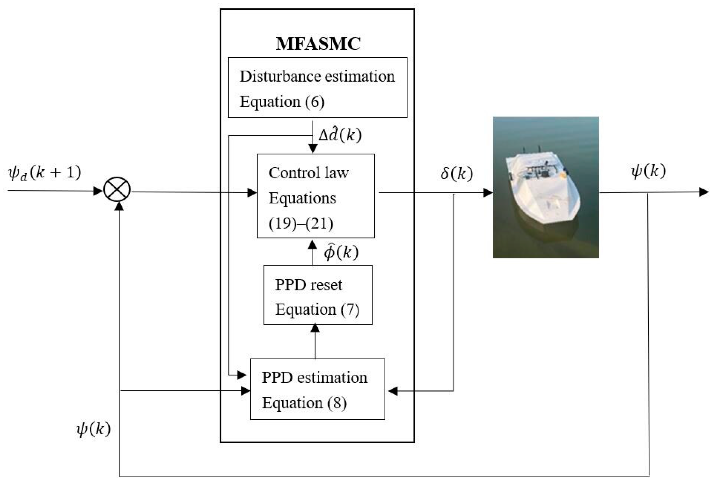
To achieve the control objective, the control algorithm is formulated with the aid of the MFAC algorithm framework, as shown in Figure 2.

In the data model (5) the control parameters $\varphi \left(k\right)$ is dynamically adjusted through the online estimation of the PPD by using the I/O data of the controlled system. The control scheme is developed using the input/output data of the controlled system, regardless of the time-varying parameters of the system. Hence, it exhibits notable robustness and adaptability. Nonetheless, the MFAC technique may not be universally applicable to all nonlinear systems. It is only effective for some classes of nonlinear systems. In [26], for USV course control systems must meet another assumption in addition to assumptions 1–3.

Quasi-Linear Assumption: For any moment $k$ and $\mathsf{\Delta }\delta \left(k\right)\ne 0$, the sign of the PPD of the system remains unchanged. This means that $\varphi \left(k\right)>\epsilon$, or $\varphi \left(k\right)<\epsilon$, where $\epsilon$ is a small positive number, $\epsilon >0$.

To adopt a classical MFAC control framework, this assumption serves as a prerequisite that the USV control system must meet to guarantee system stability. However, for the actual USV system, the course angle spans from $-{180}^{°}$ to ${180}^{°}$. So, as the rudder angle (control input) increases, it does not necessarily result in a continuous increase in the course angle (system output). The most extreme case is the process from $-{180}^{°}$ to ${180}^{°}$. To overcome this problem, the RO-CFDL-MFAC is proposed by introducing a redefined output [27]. In this paper, by combining with the discrete SMC method, the stability of the system can be ensured without the need for this assumption.

3.1. Disturbance Estimation

Since the disturbance term $∆d\left(k\right)$ of (5) is unknown, there is a need to adopt a method to handle this term. According to the disturbance estimation technique [39], it can be estimated as

$$∆\widehat{d}\left(k\right)=∆d\left(k-1\right),$$

Substituting (5) into the above equation

$$∆\widehat{d}\left(k\right)=\psi \left(k\right)-\psi \left(k-1\right)-\varphi \left(k-1\right)∆\delta \left(k-1\right),$$

(6)

Disturbance estimation error is defined as:

$$∆\tilde{d}\left(k\right)=∆\widehat{d}\left(k\right)-∆d\left(k\right),$$

Hence,

$$∆\tilde{d}\left(k\right)=∆d\left(k-1\right)-∆d\left(k\right),$$

where $∆\tilde{d}\left(k\right)$ is assumed to be bounded [39] and $\left|∆\tilde{d}\left(k\right)\right|<d_0$.

3.2. PPD Estimation

Since the system model is unavailable, time-varying parameter $\varphi \left(k\right)$ is unknown. We obtained its estimate through the minimization of cost function [17]:

$$J\left(\widehat{\varphi }\left(k\right)\right)={\left|\psi \left(k\right)-\psi \left(k-1\right)-\widehat{\varphi }\left(k\right)∆\delta \left(k-1\right)\right|}^2+\mu {\left|\widehat{\varphi }\left(k\right)-\widehat{\varphi }\left(k-1\right)\right|}^2,$$

where $\mu$ is a positive weighting factor, $\mu >0$. Hence, the estimation of the PPD is calculated

$$\widehat{\varphi }\left(k\right)=\widehat{\varphi }\left(k-1\right)+\frac{\eta ∆\delta \left(k-1\right)}{\mu +{∆\delta \left(k-1\right)}^2}\times \left(∆\psi \left(k\right)-∆\widehat{d}\left(k\right)-\widehat{\varphi }\left(k-1\right)∆\delta \left(k-1\right)\right),$$

(7)

$$\mathrm{if}\left|\widehat{\varphi }\left(k\right)\right|\le \epsilon \mathrm{or}\left|∆\delta \left(k-1\right)\right|\le \epsilon ,\widehat{\varphi }\left(k\right)=\widehat{\varphi }\left(1\right),$$

(8)

where $\epsilon >0$, $\eta \in \left(\mathrm{0,1}\right]$. $\epsilon$ is chosen as a sufficiently small positive value. The initial value of $\widehat{\varphi }\left(k\right)$ is $\widehat{\varphi }\left(1\right)$ and $\widehat{\varphi }\left(1\right)>0$.

Rewrite (5) as:

$$\psi \left(k+1\right)=\psi \left(k\right)+\left(\widehat{\varphi }\left(k\right)+\sigma \left(k\right)\right)∆\delta \left(k\right)+∆\widehat{d}\left(k\right)-∆\tilde{d}\left(k\right),$$

(9)

where $\sigma \left(k\right)=\varphi \left(k\right)-\widehat{\varphi }\left(k\right)$ is the parameter estimation error. As long as PPD $\widehat{\varphi }\left(k\right)$ remains bounded and $\left|\varphi \left(k\right)\right|\le b$, $\sigma \left(k\right)$ also stays bounded. When $\varphi \left(k\right)$ is unknown, $\sigma \left(k\right)$ cannot be accurately calculated. Thus, $\sigma \left(k\right)$ is taken as a constant $\sigma$.

3.3. Model-Free Adaptive Sliding Mode Control Law

This section discusses the aspects of designing the model-free adaptive discrete-time second-order fast terminal sliding mode controller. First of all, the system output error is defined as

$$e\left(k\right)={\psi }_d\left(k\right)-\psi \left(k\right),$$

(10)

where ${\psi }_d\left(k\right)$ is the desired signal that is assumed to be bounded.

The selection for the nonlinear fast terminal sliding surface is:

$$s\left(k\right)=e\left(k\right)+{\alpha }_{1}e\left(k-1\right)+{\alpha }_2{sig}^{\gamma }\left(e\left(k-1\right)\right)$$

(11)

where $0<{\alpha }_1<1$, $0<{\alpha }_2<1$, $0<\gamma <1$ and ${sig}^{\gamma }\left(e\left(k\right)\right)={\left|e\left(k\right)\right|}^{\gamma }sgn\left(e\left(k\right)\right)$, $sgn\left(\right)$ is signum function. The nonlinear term ${\alpha }_2{sig}^{\gamma }\left(e\left(k-1\right)\right)$ is responsible for facilitating the rapid approach of the system state to equilibrium when it is distant from that point. Meanwhile, the linear term ${\alpha }_{1}e\left(k-1\right)$ serves to expedite the convergence of the system state when it nears equilibrium.

From (11), we arrive at

$$s\left(k+1\right)=e\left(k+1\right)+{\alpha }_{1}e\left(k\right)+{\alpha }_2{sig}^{\gamma }\left(e\left(k\right)\right),$$

(12)

By introducing the high-order SMC strategy [39], second-order discrete sliding mode function is given as:

$$\overline{s}\left(k\right)=s\left(k\right)+\beta s\left(k-1\right),$$

(13)

where $-1<\beta <0$ is a design parameter.

The equivalent incremental control law of sliding mode surface can be obtained by the following:

$$∆\overline{s}\left(k+1\right)=\overline{s}\left(k+1\right)-\overline{s}\left(k\right)=0,$$

(14)

Substituting $\overline{s}\left(k+1\right)=s\left(k+1\right)+\beta s\left(k\right)$ into (14) gives

$$s\left(k+1\right)+\beta s\left(k\right)=\overline{s}\left(k\right),$$

(15)

With (12) and (15), we arrive at:

$$e\left(k+1\right)+{\alpha }_{1}e\left(k\right)+{\alpha }_2{sig}^{\gamma }\left(e\left(k\right)\right)+\beta s\left(k\right)=\overline{s}\left(k\right),$$

(16)

Substituting Equation (10) into (16), it follows that:

$${\psi }_d\left(k+1\right)-\psi \left(k+1\right)+{\alpha }_{1}e\left(k\right)+{\alpha }_2{sig}^{\gamma }\left(e\left(k\right)\right)+\beta s\left(k\right)=\overline{s}\left(k\right).$$

(17)

Considering (9) and disturbance estimation error is assumed to have vanished, i.e., $∆\tilde{d}\left(k\right)=0$. The equivalent incremental control input is obtained as:

$$∆{\delta }_{eq}\left(k\right)=\left({\psi }_d\left(k+1\right)-\psi \left(k\right)+{\alpha }_{1}e\left(k\right)+{\alpha }_2{sig}^{\gamma }\left(e\left(k\right)\right)-∆\widehat{d}\left(k\right)+\beta s\left(k\right)-\overline{s}\left(k\right)\right)/\left(\widehat{\varphi }\left(k\right)+\sigma \right).$$

(18)

The designed control law (18) comes into effect during the sliding phase when the system trajectory stays on the sliding surface. If the initial state of the system is not on the sliding surface, or the disturbance is not accurately estimated, i.e., $∆\tilde{d}\left(k\right)\ne 0$, the equivalent control is unable to drive the trajectory of the system towards the sliding surface. In order to enhance the robustness of the controller, a robust discrete SMC strategy is developed. Hence, a switching term is designed as follows:

$$\mathsf{\Delta }{\delta }_{sw}(k)=\left(q\overline{s}(k)+{\lambda }_s\mathrm{sgn}(\overline{s}(k))\right)/(\widehat{\varphi }(k)+\sigma ).$$

(19)

where the control gains are supposed to satisfy the conditions $0<q<1$ and ${\lambda }_s>d_0$.

From (18) and (19), the total incremental control input is written as:

$$∆\delta \left(k\right)=∆{\delta }_{eq}\left(k\right)+∆{\delta }_{sw}\left(k\right),$$

(20)

Finally, the proposed MFATSMC is obtained as:

$$\delta \left(k\right)=\delta \left(k-1\right)+∆\delta \left(k\right).$$

(21)

3.4. Procedure of MFASMC Design

In this part, the steps involved in implementing the proposed MFASMC controller are detailed and illustrated in Figure 3. After analyzing the contents of Section 3.1, Section 3.2 and Section 3.3, the general design procedures of the MFASMC technique can be summarized as follows.

Step 1: Initialization. The initial value of the algorithm including the initial values of PPD $\widehat{\varphi }\left(1\right)$, control input rudder $\delta \left(1\right)$ and $\delta \left(2\right)$ and parameters of MFASMC controller $\eta$, $\mu$, $\beta$, ${\alpha }_1$, ${\alpha }_2$, $\gamma$, $\sigma$, $q$, ${\lambda }_s$ are given. $k=1$.

Step 2: The system output course angle $\psi \left(k\right)$, control input rudder $\delta \left(k\right)$ and disturbance term $∆d\left(k\right)$ are got and stored. The variations $∆\psi \left(k\right)$, $\delta \left(k-1\right)$ are calculated.

Step 3: Disturbance term estimation $∆\widehat{d}\left(k\right)$ is updated.

Step 4: PPD estimation $\widehat{\varphi }\left(k\right)$ is updated by Equation (7).

Step 5: The reset algorithm (8) is used. If $\widehat{\varphi }\left(k\right)$ is close to zero, then $\widehat{\varphi }\left(k\right)$ are set to be $\widehat{\varphi }\left(1\right)$.

Step 6: The control law $\delta \left(k\right)$ is calculated by Equations (18)–(21).

Step 7: $k=k+1$.

Step 8: The determination of whether the simulation time $k$ reaches its maximum simulation time $k_{max}$ is made. If $k>k_{max}$, the simulation comes to an end. Otherwise, steps 2–7 are repeated.

4. System Stability Analysis

Theorem 2.

Considering the parameter adaptive law (7) and (8), the fast terminal sliding surface (11) and (13), along with the control input (20) using (18) and (19) for the dynamic linearization model (5), if the switching gain  ${\lambda }_s$ is selected to meet the following condition

$${\lambda }_s>d_0,$$

(22)

then, the sliding mode convergence will occur within a finite number of steps.

Proof of Theorem 2.

The proof of the Theorem 2 means that course angle $\psi$ converges to the desired ${\psi }_d$.

Substituting control laws (18)–(20) into (9) yields:

$$\psi \left(k+1\right)={\psi }_d\left(k+1\right)+{\alpha }_{1}e\left(k\right)+{\alpha }_2{sig}^{\gamma }\left(e\left(k\right)\right)+\beta s\left(k\right)-\overline{s}\left(k\right)+q\overline{s}\left(k\right)+{\lambda }_{s}sgn\left(\overline{s}\left(k\right)\right)-∆\tilde{d}\left(k\right),$$

which is substituted in (12) to give:

$$s\left(k+1\right)=-\beta s\left(k\right)+\overline{s}\left(k\right)-q\overline{s}\left(k\right)-{\lambda }_{s}sgn\left(\overline{s}\left(k\right)\right)+∆\tilde{d}\left(k\right).$$

Substituting it into (13) gives:

$$\begin{array}{c}\overline{s}\left(k+1\right)=s\left(k+1\right)+\beta s\left(k\right)\\ =\overline{s}\left(k\right)-q\overline{s}\left(k\right)-{\lambda }_{s}sgn\left(\overline{s}\left(k\right)\right)+∆\tilde{d}\left(k\right).\end{array}$$

It can be deduced that:

$$\overline{s}\left(k+1\right)-\overline{s}\left(k\right)=-q\overline{s}\left(k\right)-{\lambda }_{s}sgn\left(\overline{s}\left(k\right)\right)-∆\tilde{d}\left(k\right).$$

(23)

For (23), when $\overline{s}\left(k\right)>0$, it can be derived from (22) and (23):

$$\overline{s}\left(k+1\right)-\overline{s}\left(k\right)=-q\overline{s}\left(k\right)-{\lambda }_s-∆\tilde{d}\left(k\right).$$

Which satisfies the inequality (24):

$$-q\overline{s}\left(k\right)-{\lambda }_s-d_0<\overline{s}\left(k+1\right)-\overline{s}\left(k\right)<0,$$

(24)

when $\overline{s}\left(k\right)<0$, it can be also derived from (22) and (23):

$$\overline{s}\left(k+1\right)-\overline{s}\left(k\right)=-q\overline{s}\left(k\right)+{\lambda }_s-∆\tilde{d}\left(k\right),$$

which satisfies the inequality:

$$0<\overline{s}\left(k+1\right)-\overline{s}\left(k\right)<-q\overline{s}\left(k\right)+{\lambda }_s+d_0.$$

(25)

Considering both (24) and (25), it is obtained that

$$\left\{\begin{array}{cc}\overline{s}\left(k+1\right)<\overline{s}\left(k\right)& \overline{s}\left(k\right)>0,\\ \overline{s}\left(k+1\right)>\overline{s}\left(k\right)& \overline{s}\left(k\right)<0.\end{array}\right.$$

So, the relationship between $\overline{s}\left(k+1\right)$ and $\overline{s}\left(k\right)$ is obtained as:

$$\left|\overline{s}\left(k+1\right)\right|<\left|\overline{s}\left(k\right)\right|.$$

(26)

Equation (26) can also be written in the following:

$$\begin{gathered} \left(\overline{s}\left(k+1\right)-\overline{s}\left(k\right)\right)sgn\left(\overline{s}\left(k\right)\right)<0, \\ \left(\overline{s}\left(k+1\right)+\overline{s}\left(k\right)\right)sgn\left(\overline{s}\left(k\right)\right)>0. \end{gathered}$$

The relationship (26) is a sufficient condition that is adequate to establish the existence and arrival of a quasi-sliding mode [40]. Thus, under the action of control (17)–(19) second-order discrete sliding mode $\overline{s}\left(k\right)$ decreases monotonously, and the quasi-sliding mode is reached within limited steps.

When the second-order sliding surface $\overline{s}\left(k\right)$ enters the quasi-sliding mode, it is obtained:

$$s\left(k\right)=-\beta s\left(k-1\right).$$

Since $\beta \in \left(\mathrm{0,1}\right)$, by employing Equation (12) to achieve convergence within a finite number of steps, it can be deduced that $s\left(k\right)=0$.

Based on the above analysis, if $s\left(k\right)=0$, form (10) we arrive at

$$e\left(k\right)=-{\alpha }_{1}e\left(k-1\right)-{\alpha }_2{sig}^{\gamma }\left(e\left(k-1\right)\right).$$

(27)

From (27), it is easy to conclude that in a finite number of steps $e\left(k\right)$ tends towards 0. Hence, the output of the system $\psi$ will eventually converge to the desired course angle ${\psi }_d$. □

5. Simulation Research

In this section, to validate the reliability and effectiveness of the proposed control strategy, the proposed MFASMC is simulated in MATLAB 2021b. On the basis of the theory of ship maneuverability, the nonlinear Norrbin model is used. According to the continuous system [41,42] and Equation (1), the discrete mathematical representation of the USV course control system can be expressed as

$$\left\{\begin{array}{l}\psi \left(k+1\right)=\psi \left(k\right)+T_{s}r\left(k\right),\\ r\left(k+1\right)=r\left(k\right)+T_s\left(\left(K\delta \left(k\right)-\alpha r^3\left(k\right)-r\left(k\right)\right)/T+d\left(k\right)\right).\end{array}\right.$$

(28)

where $T_s$ is the sampling time. $T_s=0.1\mathrm{s}$. It should be noted that the above discrete USV course system is only used to obtain the output and input values of the USV course system in the simulation, not used in the design process of the controller.

Considering the nonlinear ship model investigated by the ‘‘Lanxin’’ USV of Dalian Maritime University [9], the parameters for the nonlinear Norrbin model are outlined as follows $k=0.701$, $T=0.332$, $\alpha =0.001$.

The initial states include course angle $\psi \left(1\right)=\psi \left(2\right)=0^{°}$, and angular velocity $r\left(1\right)=r\left(2\right)=0^{°}/\mathrm{s}$. The desired course angle is set as ${\psi }_d={60}^{°}$. To ensure equitable comparison in the subsequent analysis, the controllers’ parameters are manually fine-tuned for better performance. The proposed MFASMC parameters are $\eta =0.1$, $\mu =1$, $\beta =-0.1$, ${\alpha }_1=0.4$, ${\alpha }_2=0.1$, $\gamma =0.7$, $\sigma =0.5$, $q=0.6$, ${\lambda }_s=0.0001$, the increment PID controller parameters are $k_p=2$, $k_I=0.1$, $k_d=0.1$, and the typical MFASMC [32] controller parameters are $\eta =0.1$, $\mu =1$, $\sigma =0.5$, $q=0.6$, ${\lambda }_s=0.0001$.

To evaluate the effectiveness of the proposed controller and the comparative controllers, the mean squared error (MSE) is employed to calculate the mean of the squared difference between the actual value and the desired value of the course angle. The utilization of the mean squared error (MSE) allows for the quantification of the controller’s performance by assessing the tracking error. The Euclidean norm is equivalent to the square root of the total sum of the squares of each component within the vector. Hence, the Euclidean norm serves as a measure to assess the extent of control effort exerted by the controllers. The accuracy of the controller can be evaluated more intuitive and lucid manner by the following:

$$\begin{gathered} \mathrm{M}\mathrm{S}\mathrm{E}\left(\psi \right)=\frac{{\sum }_{i=1}^n{\left({\psi }_d-\psi \right)}^2}{n}, \\ E\left(\delta \right)=\sqrt{{\left|{\delta }_1\right|}^2+\cdots +{\left|{\delta }_n\right|}^2}. \end{gathered}$$

5.1. Simulation for the Case with Disturbance

Firstly, to verify the robust ability of the controller against disturbance $d\left(k\right)$ in the system, the following simulation is carried out. As in [8], the external time-varying disturbance of the USV system, which is caused by wind, waves and currents, is set as:

$$d\left(t\right)=2\times \left(0.1+0.1\mathit{cos}\left(0.3t\right)+0.1sin\left(0.5t\right)\right).$$

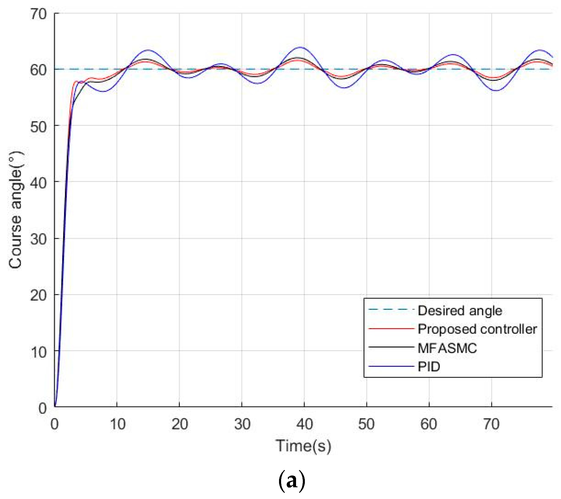
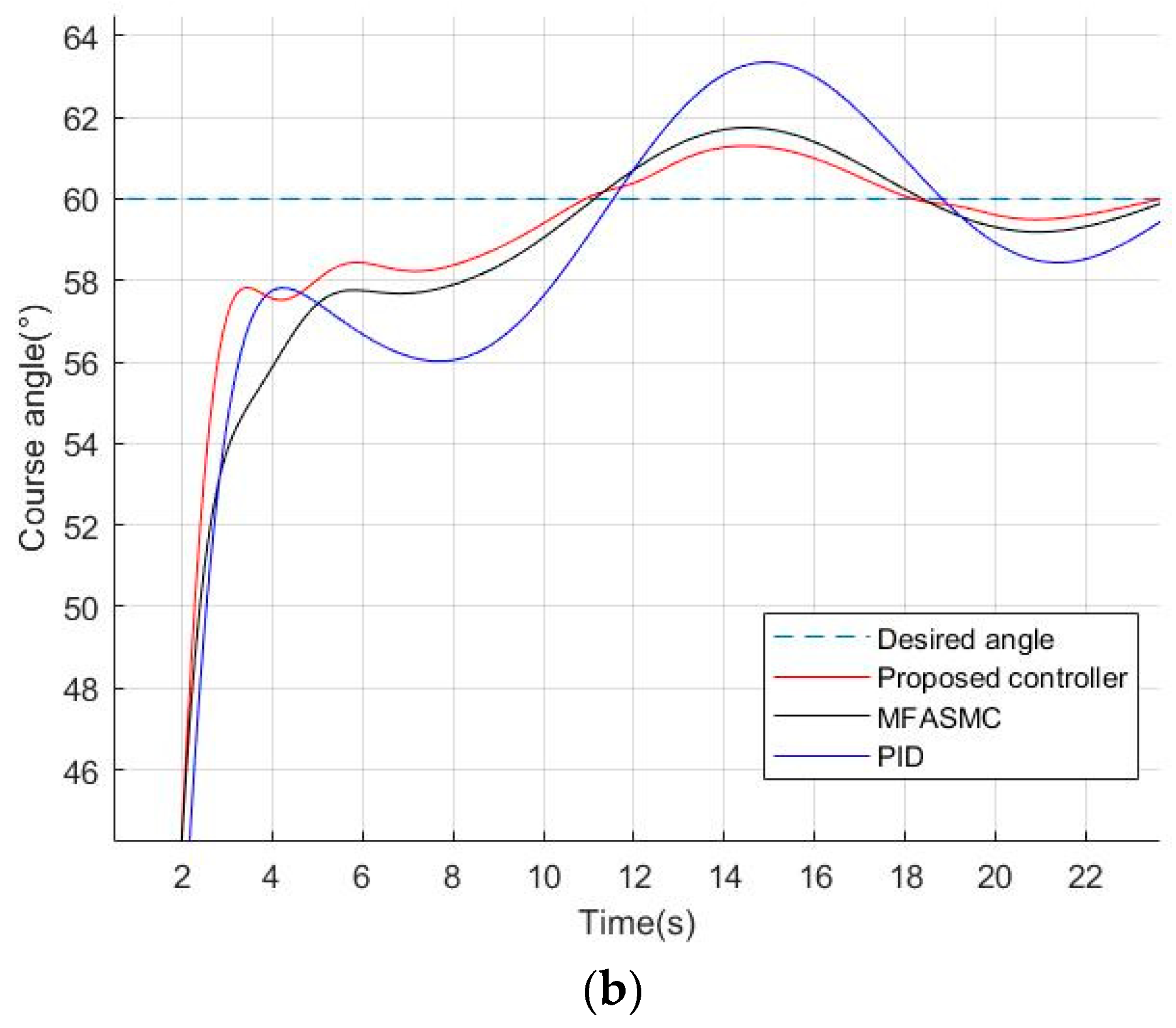
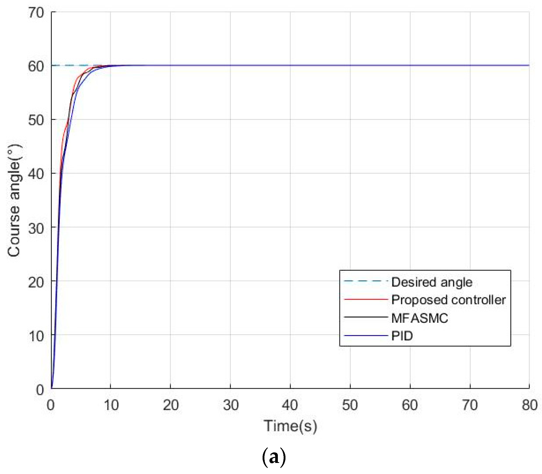
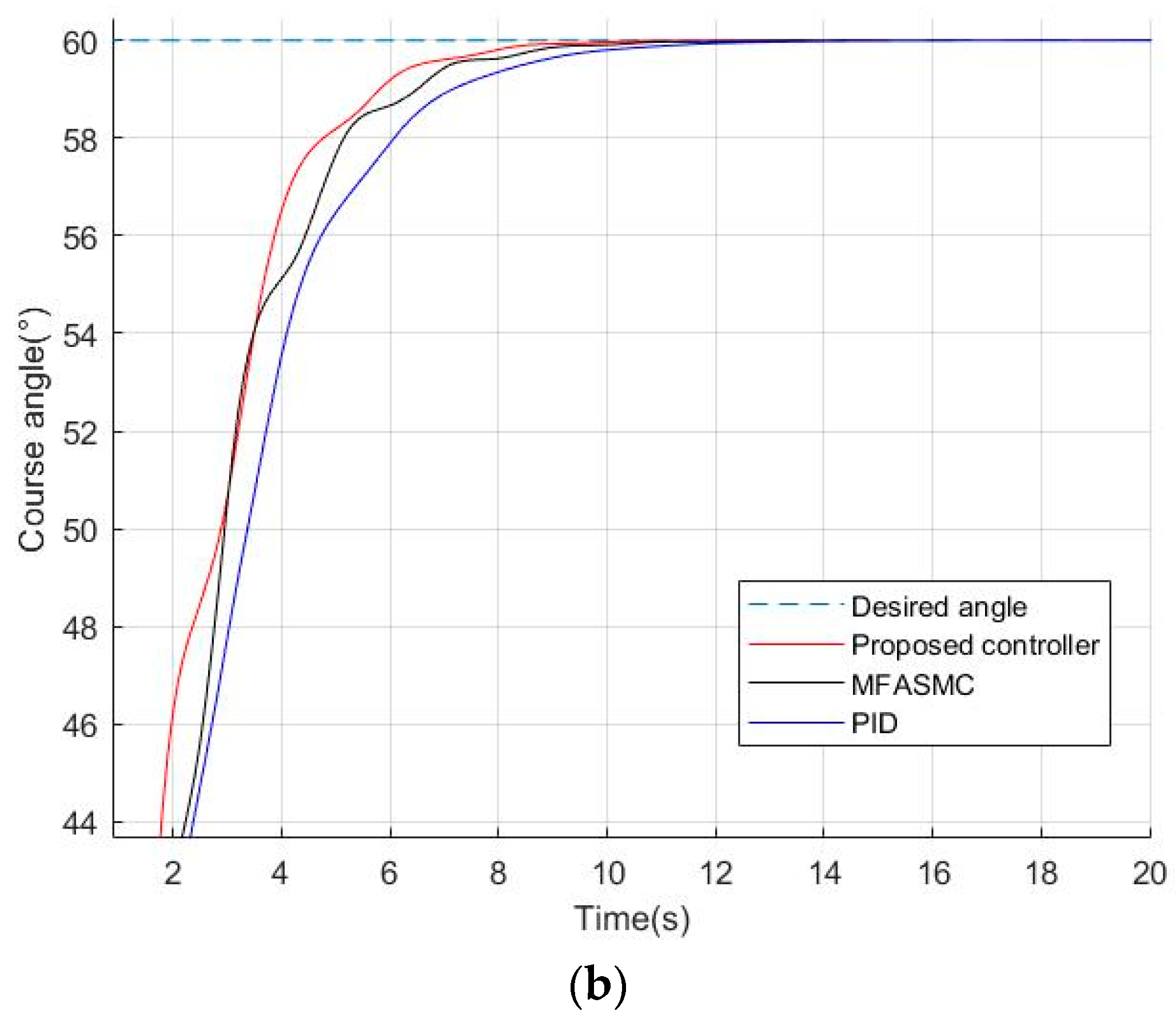
The initial states of the course control system and the control parameter are written above. Figure 4 illustrates the simulation outcomes concerning course angle control with the involvement of the three distinct controllers.

Utilizing the mean squared error of the course angle tracking error to compare the control performance of the controllers, the MSE values of the tracking error are calculated and shown in

Table 1. Comparison of simulation results for the case with disturbance.

Controller	MSE1 ($\mathit{\psi }$)	MSE2 ($\mathit{\psi }$)	E1 ($\mathit{\delta }$)	E2 ($\mathit{\delta }$)
PID	0.2633	0.0014	1.9353	3.9260
MFASMC	0.2408	4.0905 × 10−4	2.0853	3.7221
Proposed	0.2482	2.0888 × 10−4	2.2066	3.7158

. MSE1 and $E1$ represent the MSE value and Euclidean norm value for the entire simulation time from 0 s to 5 s. MSE2 and $E2$ represent the MSE value and Euclidean norm value for the part simulation time from 5 s to 80 s. As can be seen from Figure 4, and the MSE1 and MSE2 in Table 1, the MSE2 by the proposed method is smaller, while the MSE1 by MFASMC is smaller. It shows that the tracking response ability of the heading angle is slightly weak under the proposed method in comparison with the MFASMC. Simultaneously, the conclusion is made that the proposed method can better resist external disturbances in the process of course-keeping. 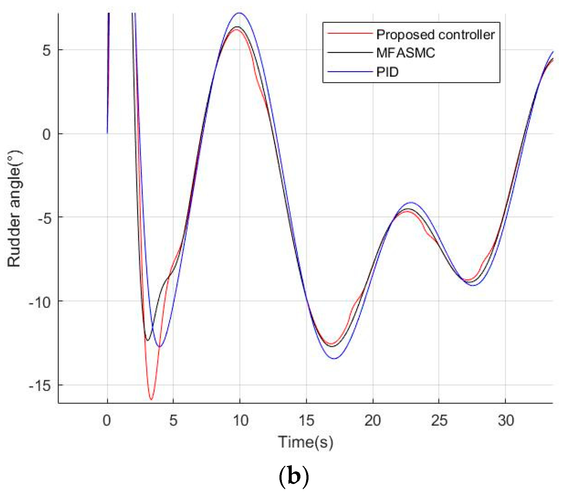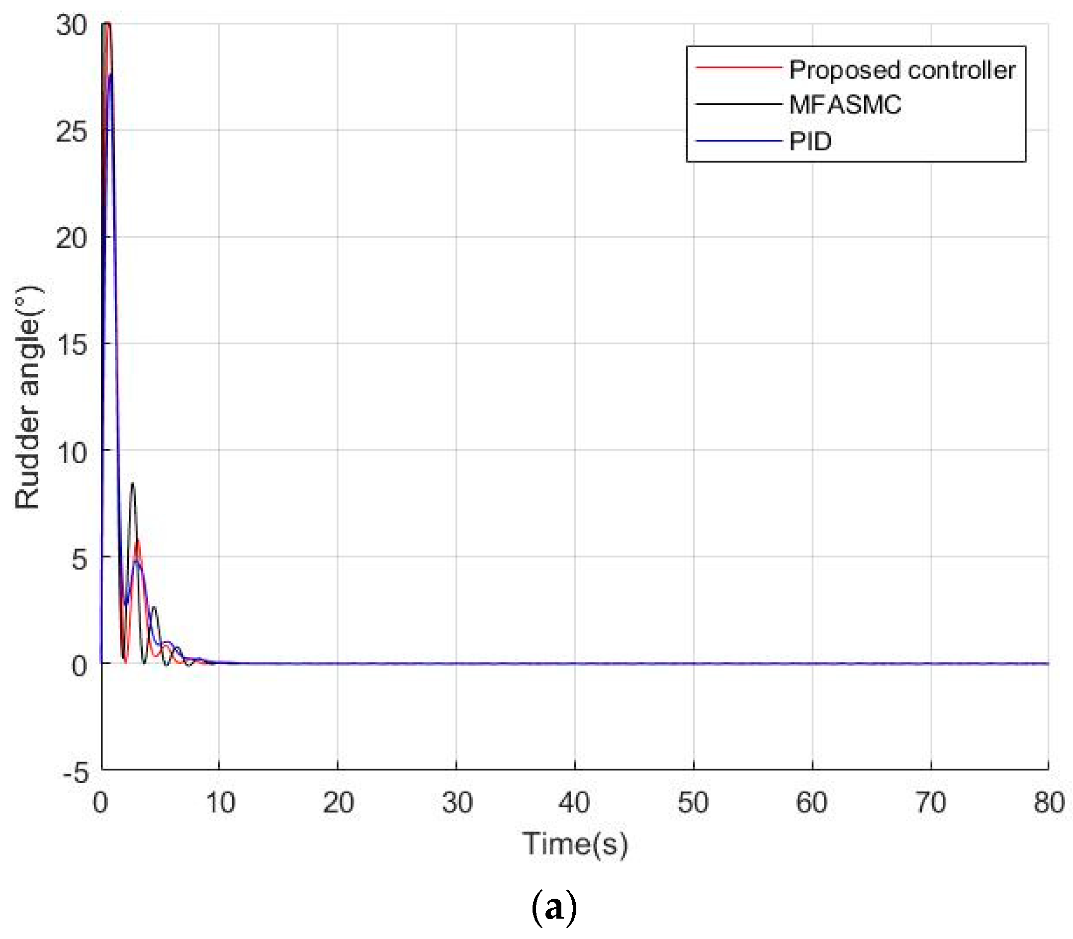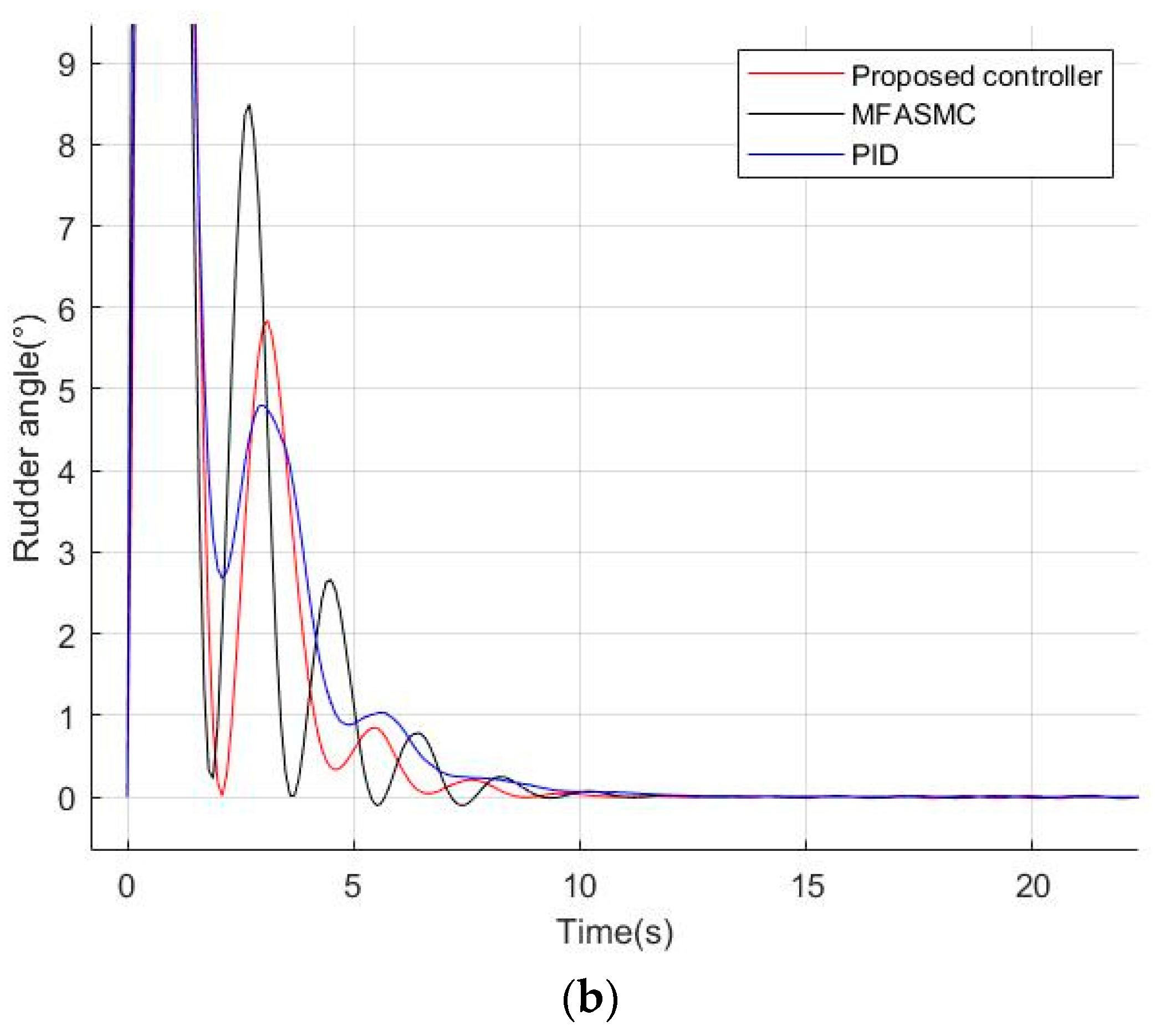Figure 5 represents the comparison between the rudder angles given by controllers. The control performance of the PID controller is significantly worse, and its anti-disturbance ability is poor. Using the proposed controller USV has a smaller error and rudder angle to track the desired course angle.

5.2. Simulation for the Case with Uncertainty

In Equation (28) the parameter perturbation $∆K$ can be transformed into an equivalent one $d\left(k\right)=∆K\delta \left(k\right)/T$. For the purpose of assessing robustness in systems afflicted by parameter uncertainty, simulations are carried out in this part. The initial states are not changed except ${\alpha }_2=0.1$. The remaining simulation conditions are configured as follows: the parameter $K$ in Equation (28) is subjected to variation to emulate the perturbation stemming from stochastic model parameters, i.e., the parameter $K$ is assigned a random variable value, $K=\left(1+2\times rand\left(1\right)\right)\times 0.701$. MATLAB function $rand\left(1\right)$ is used to generate the random numbers from 0 to 1.

The comparative simulation results are illustrated in Figure 6. The MSE values of the course angle tracking error are calculated and displayed in

Table 2. Comparison of simulation results for the case with uncertainty.

Controller	MSE1 ($\mathit{\psi }$)	MSE2 ($\mathit{\psi }$)	E1 ($\mathit{\delta }$)	E2 ($\mathit{\delta }$)
PID	0.2601	5.4909 × 10−5	1.4147	0.0661
MFASMC	0.2360	2.0384 × 10−5	1.6714	0.0456
Proposed	0.2318	1.1460 × 10−5	1.5711	0.0432

.

In such a case, from Figure 6 and Figure 7 and MSE values in Table 2, the difference in the control performance of the three controllers is not significant. Under the action of three controllers, the heading angle quickly tracks the desired value. By the compassion of MSE1 and MSE2, the MFASMC has a bigger value than the proposed controller. Meanwhile, in terms of energy consumption, the values of $E1$ and $E2$ by the proposed method are the smallest of the three controllers. This means the proposed controller has faster tracking speed to the desired angle and better performance on the course keeping in the case of parameter perturbation. Figure 7 represents the comparison of system control rudder angles given by controllers.

6. Conclusions

In the article, the focus is directed toward addressing the challenge of USV course control with disturbance. To tackle this issue, a novel model-free approach is employed by integrating the second-order discrete sliding mode function and the fast terminal sliding mode surface with the CFDL-MFAC theory. Furthermore, the disturbance effect is considered and the method is used to estimate the disturbance in the controller design process. A theoretical analysis provides a solid foundation for ensuring the guaranteed convergence of the closed-loop system, even when subjected to disturbances. Hence, the tracking error between the output of the controlled system and a desired one can converge towards a compact vicinity surrounding the origin. Comparative simulations verify the effectiveness and superiority of the proposed control approach. Through simulations, it is evident that the proposed MFASMC algorithm outperforms both the MFASMC and PID methods. Notably, the novel MFASMC algorithm displays remarkable insensitivity to system disturbances and parameter perturbations, consistently delivering superior control performance.

In the future, different control methods will be tested on the physical USV to assess the tracking performance of the proposed scheme. Meanwhile, the action implementation of the actuator will be discussed, such as the dynamics of rudders or propellers, actuator saturation and actuator fault. Besides, as the tracking performance of the proposed method relies on the accuracy of input and output data, research will be conducted on how to deal with noise in the measurement data.