Distributed Dual Closed-Loop Model Predictive Formation Control for Collision-Free Multi-AUV System Subject to Compound Disturbances

Abstract

This paper focuses on the collision-free formation tracking of autonomous underwater vehicles (AUVs) with compound disturbances in complex ocean environments. We propose a novel finite-time extended state observer (FTESO)-based distributed dual closed-loop model predictive control scheme. Initially, a fast FTESO is designed to accurately estimate both model uncertainties and external disturbances for each subsystem. Subsequently, the outer-loop and inner-loop formation controllers are developed by integrating disturbance compensation with distributed model predictive control (DMPC) theory. With full consideration of the input and state constraints, we resolve the local information-based DMPC optimization problem to obtain the control inputs for each AUV, thereby preventing actuator saturation and collisions among AUVs. Moreover, to mitigate the increased computation caused by the control structure, the Laguerre orthogonal function is applied to alleviate the computational burden in time intervals. We also demonstrate the stability of the closed-loop system by applying the terminal state constraint. Finally, based on a connected directed topology, comparative simulations are performed under various control schemes to verify the robustness and superior performance of the proposed scheme.

1. Introduction

Autonomous underwater vehicles (AUVs) have assumed indispensable roles in various underwater operations, such as ocean exploration and hydrologic surveys [1]. They can autonomously perform appropriate maneuvers to achieve predefined objectives. Compared with the operational capability of a single AUV, collaborative AUVs can respond more reliably and flexibly to complex missions and extended operational ranges, thereby improving the efficiency and robustness of undersea operations. Given this backdrop, numerous application cases about AUV coordinated formation have been triggered in both civilian and industrial fields for decades [2,3]. Irrespective of the specific collaborative missions undertaken by AUVs, the core challenge lies in ensuring motion stability of AUV formations within complex underwater environments and the constraints of their own models. To tackle this problem, several mainstream methodologies have been proposed by engineers and academics. Studies by Chen et al. [4] and Zhen et al. [5] proposed AUV formation control schemes combined with the virtual structure method. However, this approach suffers from limited flexibility and applicability. Wang et al. [6] utilized the leader–follower method to address the AUV formation tracking problem, but this approach relies on the state of the leader, reducing the robustness and fault tolerance of the formation. Conversely, leaderless formations have been proposed promisingly and have received more considerable attention [7]. Munir et al. [8] proposed a new arbitrary-order distributed control strategy based on the novel sliding surfaces of error dynamics, which addresses the cooperative tracking control of uncertain higher-order nonlinear systems. The strategies to mitigate the chattering issue caused by sliding surfaces are discussed in [9]. Despite the abundance of existing research, multiple-AUV formation tracking control remains a significantly challenging project.

One of the main challenges is the various disturbances resulting from the underwater environment and the motion model of the AUVs themselves [10]. On the one hand, unknown disturbances such as waves, tides, and currents, are inevitable in practical marine environments. On the other hand, AUVs exhibit highly nonlinear and coupled dynamics, leading to model uncertainties. These uncertainties are often induced by modeling errors and deviations in hydrodynamic coefficient measurement. According to the research by Cui et al. [11], these external disturbances and model uncertainties that degrade the system performance negatively are referred to as compound disturbances. In response to these challenges, researchers have developed diverse schemes, such as disturbance observers [12], fuzzy logic theory [13], and neural networks [14]. Among these, the extended state observer (ESO) initially proposed by Han [15] is an attractive option to estimate compound disturbances, as it does not rely on an accurate model. Lei et al. [16] designed a high-gain ESO to solve AUV horizontal trajectory tracking problems under the time-varying disturbances. Although many ESOs have been established for different platforms, most only guarantee asymptotic convergence of estimation errors, implying a potentially infinite convergence time. Some research works also lack a rigorous analysis of convergence. Considering the impact of severe underwater environments on estimation accuracy, the concept of finite-time ESO proves more beneficial for improving control performance [17]. Wang et al. [18] implemented a FTESO-based nonsingular terminal sliding mode controller to address unmanned surface vehicle (USV) trajectory tracking in disturbed environments. This approach ensured that the disturbance estimation errors converge within a finite time. However, there remains room for improvement and optimization of the design structure to further enhance observation performance.

AUV formation navigation also presents significant technical challenges due to various complex constraints. For instance, the AUV attitude has a certain desired range and navigation velocities are inherently limited. These intrinsic input and state constraints pose substantial challenges to control performance [19]. In practical applications, actuators often have input saturation constraints due to physical structure limitations. This results in a limitation of the actual active control force of the AUV. If a control signal exceeds this boundary, it may lead to system instability. However, most previous work assumes that the actuators can tolerate any level of control signals. To avoid actuator saturation, a nonlinear auxiliary system for filtering saturation errors was proposed [20]. Additionally, collisions between AUVs are undesirable during the formation configuration phase. Thus, the ability to avoid collisions is vital for AUV formation control. A wealth of solutions have been developed to this end, with Li and Wang [21] proposing a collision-free position consensus algorithm for AUVs based on potential function. Moreover, Xu et al. [22] presented an event-triggered algorithm based on deep reinforcement learning to avoid AUV collisions. However, the above studies disregard the physical constraints of AUVs. From the perspective of safe navigation, it is essential to integrate factors such as input, state restrictions, and collision avoidance into the design scheme.

Model predictive control (MPC) has garnered considerable attention due to its ability to simultaneously handle multiple composite constraints and offer superior dynamic performance. This is widely applied to MIMO systems affected by model distortions and complex constraints. Several MPC-based applications have been integrated into AUV control systems. Zhang et al. [23] proposed an MPC-based AUV trajectory tracking strategy under random disturbances. In [24], a robust model-predictive control scheme based on the active disturbance rejection control approach was developed for the AUV tracking task. The challenge of extending these systems to multi-AUV systems involves coordinating the control behavior of each subsystem and ensuring the closed-loop stability of the local MPC optimization problem under system constraints. This coordination aims to maximize the overall control performance. Hence, DMPC came into being. Zheng et al. [25] proposed a DMPC method based on local state information for MAS formation tracking. To the best of our knowledge, there are few studies that apply DMPC to multi-AUV formations. Wei et al. [26] developed a Lyapunov-based distributed predictive controller for AUV formation tracking, subject to current disturbances. The auxiliary controller was utilized to establish stability constraints to ensure the closed-loop stability of the system. However, this method only considers horizontal formations without uncertainties and state constraints. Furthermore, many works that design predictive controllers result in additional computational loads, which could impair the real-time execution capability of the controller. Shen and Shi [27] managed to reduce the MPC computational burden by decomposing the original AUV trajectory tracking optimization problem into smaller subproblems and then solving them in a distributed manner. Despite these efforts, there has been no research to address the heavy computation of DMPC applied to AUV formations. In order to improve the dynamic response and control accuracy of AUV formation tracking in three-dimensional (3-D) space, we adopt the Laguerre orthogonal function to reduce the computational load. In response to these discussions, it is imperative to develop a safe and efficient formation control scheme to solve the problems of disturbances, parameter uncertainties, and complicated constraints.

Motivated by the above observations, this paper investigates the collision-free formation tracking of multi-AUVs with compound disturbances under complicated constraints. A novel FTESO-based distributed dual closed-loop model predictive control scheme is proposed. This method satisfies the formation constraints and collision avoidance requirements while compensating for model uncertainties and external disturbances. We incorporate the Laguerre function to alleviate the computational burden of the DMPC optimization problem, also giving corresponding stability analysis. Based on the connected directed topology, comparative simulations under different schemes demonstrate the effectiveness and robustness of our proposed scheme. The main contributions of this paper are as follows:

• Compared with the FTESO-based controllers presented in works [16,28], the proposed third-order fast FTESO can estimate the compound disturbances and their first derivatives, which effectively suppress the amplification and fluctuation of the generalized uncertainties. It has better estimation accuracy and convergence speed. Hence, the active disturbance rejection capability of AUV formation is enhanced;
• Unlike the existing DMPC schemes depicted in works [29,30], a dual closed-loop structure is utilized to enhance the response speed of the DMPC system and the controllability of the AUV speed. The outer-loop controller sets the desired velocity and the inner-loop controller generates the driving force. By solving the constrained quadratic programming (QP) problems, the risks of actuator saturation and collision are reduced. The safety and robustness of formation tracking are improved;
• In order to solve the issue of heavy computational burden in traditional predictive control, the Laguerre orthogonal function is incorporated to reconstruct the input matrices, which automatically trades off control performance and computational complexity, thus avoiding possible formation deviation due to slow computational speed. The stability of the closed-loop system is proved by exerting terminal state constraints.

The rest of this paper is organized as follows: Section 2 introduces some notations, lemmas, and graph theory, and describes the AUV model and control objective. Section 3 presents the methodology, including the design of the FTESO and dual closed-loop DMPC scheme, the application of the Laguerre function, and the corresponding stability analysis. Section 4 and Section 5, respectively, provide simulation results and conclusions.

2. Preliminaries

2.1. Notations and Lemmas

Notation. 

${ℝ}^n$ represents the n-dimensional Euclidean space, and ${ℝ}^{m\times n}$ denotes the set of $\left(m\times n\right)$ real matrix. $I_n$, $0_n$, and $0_{p\times q}$ signify $\left(n\times n\right)$ identity matrix, $\left(n\times n\right)$, and $\left(p\times q\right)$ null matrices, respectively. $‖·‖$ refers to the Euclidean vector norm and the induced matrix norm, while the infinity norm is denoted by ${‖·‖}_{\infty }$. ${\lambda }_{\min }\left(·\right)$ represents the minimum eigenvalue of the specified matrix $\left(·\right)$, with its maximum eigenvalue denoted as ${\lambda }_{\max }\left(·\right)$. For simplicity, some notations are defined as $si{g}^p\left(x\right)=\mathrm{sign}\left(x\right){\left|x\right|}^p$, ${\left|x\right|}^p={\left[{\left|x_1\right|}^p,{\left|x_2\right|}^p,\dots ,{\left|x_n\right|}^p\right]}^T$, $x={\left[x_1,x_2,\dots ,x_n\right]}^T$, $p\in ℝ$. $\mathrm{sign}\left(·\right)$ symbolizes the signum function with $\mathrm{sign}\left(0\right)=0$. Notably, $si{g}^0\left(x\right)=\mathrm{sign}\left(x\right)$, $si{g}^0\left(x\right){\left|x\right|}^p=si{g}^p\left(x\right)$.

Lemma 1 

([31]). Consider the system $\dot{x}\left(t\right)=f\left(x\left(t\right)\right)$, $x\left(0\right)=x_0$, $f\left(0\right)=0$, $x\in {ℝ}^n$, where $f:U\to {ℝ}^n$ is a continuous function. Suppose that this system has a unique solution in forward time for all initial conditions. If there exists a Lyapunov function $V\left(x\right)$, with $V\left(x_0\right)$ denoting its initial value, the following can be assumed: (1) The trajectory of this system is finite-time uniformly ultimately bounded stable within the region of $Q_1=\left\{\left.x\right|V{\left(x\right)}^{{\alpha }_1-{\alpha }_2}<\frac{{\beta }_2}{{\mathsf{\gamma }}_1}\right\}$, if $\dot{V}\left(x\right)\le -{\beta }_{1}V{\left(x\right)}^{{\alpha }_1}+{\beta }_{2}V{\left(x\right)}^{{\alpha }_2}$ for ${\alpha }_1>{\alpha }_2$, ${\beta }_1>0$, ${\beta }_2>0$, ${\mathsf{\gamma }}_1\in \left(0,{\beta }_1\right)$. The settling time for the states reaching the stable residual set is subject to the constraint as $T_1\le \frac{V{\left(x_0\right)}^{1-{\alpha }_1}}{\left({\beta }_1-{\mathsf{\gamma }}_1\right)\left(1-{\alpha }_1\right)}$. (2) The trajectory of this system is fast finite-time uniformly ultimately bounded stable within $Q_2=\left\{\left.x\right|{\mathsf{\gamma }}_{1}V{\left(x\right)}^{{\alpha }_1-{\alpha }_2}+{\mathsf{\gamma }}_{2}V{\left(x\right)}^{1-{\alpha }_2}<{\beta }_3\right\}$, if $\dot{V}\left(x\right)\le -{\beta }_{1}V{\left(x\right)}^{{\alpha }_1}-{\beta }_{2}V\left(x\right)+{\beta }_{3}V{\left(x\right)}^{{\alpha }_2}$ for ${\beta }_3>0$, ${\mathsf{\gamma }}_2\in \left(0,{\beta }_2\right)$. The convergence time T₂ is bounded as $T_2\le \frac{\ln \left[\left({\beta }_2-{\mathsf{\gamma }}_2\right)V{\left(x_0\right)}^{1-{\alpha }_1}/\left({\beta }_1-{\mathsf{\gamma }}_1\right)+1\right]}{\left({\beta }_2-{\mathsf{\gamma }}_2\right)\left(1-{\alpha }_1\right)}$.

2.2. Graph Theory

We introduce a directed topology graph $G=\left\{V,\epsilon \right\}$ to describe the information interactions among the AUVs. Let the node set $V=\left\{V_1,V_2,\cdots ,V_N\right\}$ to represent the N members in the formation, and an edge set $\epsilon \subseteq V\times V$ to represent the communication from the node $V_i$ to the node $V_j$. $A=\left[a_{ij}\right]\subset {ℝ}^{N\times N}$ is defined as an adjacency matrix, where $a_{ij}$ represents the connection weight and $a_{ij}=1$ if $\left(i,j\right)\in \epsilon$, while $a_{ij}=0$ if $\left(i,j\right)\notin \epsilon$. It is assumed that the ith vehicle could receive information from the virtual leader and its neighbors ${\mathrm{N}}_i=\left\{j\in V:\left(j,i\right)\in \epsilon \right\}$. The graph is termed an undirected graph if bidirectional communication links exist among all members of the formation. Otherwise, it is referred to as a directed graph. A directed graph is considered strongly connected if a directed path can connect any point in the formation to any other.

2.3. AUV Model

As shown in Figure 1, it is convenient to describe the six-degree-of-freedom (DOF) AUVs with two reference frames: an earth-fixed frame $\left\{E\right\}$ and a body-fixed frame $\left\{B\right\}$. This paper employs a fully actuated torpedo-type AUV, referenced from [32], based on the control objectives. In addition, the AUV uses an ultra-short baseline acoustic positioning system for underwater localization. Since this AUV can be regarded as a highly metacentric stable vehicle with self-stable roll motion, the effect of roll is ignored (roll angle ${\varphi }_i=0$, roll angular velocity $p_i=0$). The kinematics and dynamics of the ith AUV are described as follows [33]:

$${\dot{\eta }}_i=J\left({\eta }_i\right)v_i$$

(1)

$$M_i{\dot{v}}_i+C_i\left(v_i\right)v_i+D_i\left(v_i\right)v_i+g_i\left({\eta }_i\right)={\tau }_i+{\tau }_{ic}$$

(2)

where $i=1,2,\dots ,N$, ${\eta }_i={\left[x_i,y_i,z_i,{\theta }_i,{\psi }_i\right]}^T\in {ℝ}^5$, and $v_i={\left[u_i,v_i,w_i,q_i,r_i\right]}^T\in {ℝ}^5$ denote the states of position, orientation, and velocity of the AUV, respectively. $J\left({\eta }_i\right)$ is a rotation transformation matrix from the body-fixed frame to the earth-fixed frame, expressed as:

$$J\left({\eta }_i\right)=\left[\begin{array}{ccccc}\cos {\psi }_i\cos {\theta }_i& -\sin {\psi }_i& \cos {\psi }_i\sin {\theta }_i& 0& 0\\ \sin {\psi }_i\cos {\theta }_i& \cos {\psi }_i& \sin {\psi }_i\sin {\theta }_i& 0& 0\\ -\sin {\theta }_i& 0& \cos {\theta }_i& 0& 0\\ 0& 0& 0& 1& 0\\ 0& 0& 0& 0& 1/\cos {\theta }_i\end{array}\right]$$

(3)

$M_i$ represents the inertial matrix, which includes added mass. $C_i\left(v_i\right)$ and $D_i\left(v_i\right)$ denote the Coriolis and centripetal and hydrodynamic damping matrix, respectively, while $g_i\left({\eta }_i\right)$ represents the restoring force and moment generated by gravity and buoyancy. ${\tau }_i={\left[{\tau }_{iu},{\tau }_{iv},{\tau }_{iw},{\tau }_{iq},{\tau }_{ir}\right]}^T$ represents the control input, and ${\tau }_{ic}$ denotes the external disturbance. Detailed expressions of these matrices are available in [34].

In practical engineering, we may not be able to obtain accurate hydrodynamic coefficients in the model, so the matrices in (2) are typically divided into two parts: the nominal value part and the uncertainty part caused by linear shifts, i.e., $M_i=M_i^{\ast }+\Delta M_i$, $C_i\left(v_i\right)=C_i^{\ast }\left(v_i\right)+\Delta C_i\left(v_i\right)$, $D_i\left(v_i\right)=D_i^{\ast }\left(v_i\right)+\Delta D_i\left(v_i\right)$, and $g_i\left({\eta }_i\right)=g_i^{\ast }\left({\eta }_i\right)+\Delta g_i\left({\eta }_i\right)$, where ${\left(·\right)}_i^{\ast }$ denotes the nominal value that can be obtained from the computational fluid dynamics (CFD) or experimental analysis. $\Delta {\left(·\right)}_i$ symbolizes the difference between the real value and the nominal value.

Accordingly, the ith AUV dynamic model (2) can be reformulated as:

$$M_i^{\ast }{\dot{v}}_i=-C_i^{\ast }\left(v_i\right)v_i-D_i^{\ast }\left(v_i\right)v_i-g_i^{\ast }\left({\eta }_i\right)+{\tau }_i+{\tau }_{id}$$

(4)

where ${\tau }_{id}={\tau }_{ic}-\Delta M_i{\dot{v}}_i-\Delta C_i\left(v_i\right)v_i-\Delta D_i\left(v_i\right)v_i-\Delta g_i\left({\eta }_i\right)$ is regarded as the compound disturbance, which includes uncertainties and unknown external disturbance. Typically, external disturbances are periodically varying and energy limited. The model uncertainties are related to the actual states and physical properties of the AUV. Based on the constraints of DMPC on the system state, in practice, we give the following reasonable assumption:

Assumption 1 

([11]). The ocean current disturbance term ${\tau }_{ic}$ and the first time derivative ${\dot{\tau }}_{ic}$ are bounded, and the model uncertainties $\Delta M_i$, $\Delta C_i$, $\Delta D_i$, and $\Delta g_i$ are unknown and bounded. Hence, the compound disturbance ${\tau }_{id}$ of the ith AUV is bounded and satisfies $‖{\tau }_{id}‖\le {\overline{\tau }}_{id}$, where ${\overline{\tau }}_{id}\in {ℝ}^{+}$ represents the unknown upper bound.

It should be noted that the above assumption is untenable if there are no system state constraints [35,36].

2.4. Control Objective

In this paper, the control objective is to develop a control scheme that enables AUV formation to track a reference trajectory while maintaining a predefined configuration. Initially, a FTESO is designed to compensate for external disturbances and model uncertainties of the AUV formation, so that the estimation errors converge to the origin. Subsequently, a dual closed-loop DMPC controller is designed. In this structure, the outer-loop controller enables the ith AUV to track the reference trajectory ${\eta }_r$ by generating the desired velocity, resulting in the convergence of position tracking errors. The inner-loop controller is used to achieve the convergence of velocity tracking errors. The desired formation is implemented by setting the corresponding formation configuration vector $r_{if}$ and the relative distance vector $r_{ij}$. The task must adhere to various constraints and ensure collision avoidance. Because the navigation trajectory has a limited range and the speed is continuous without abrupt changes, we adopt the following reasonable assumptions to avoid singularities in the reference trajectory:

Assumption 2. 

The reference trajectory ${\eta }_r={\left[x_r,y_r,z_r,{\theta }_r,{\psi }_r\right]}^T$ and its derivatives are smooth and bounded, i.e., ${‖{\eta }_r‖}_{\infty }\le {\overline{\eta }}_r$, ${‖{\dot{\eta }}_r‖}_{\infty }\le {\overline{\eta }}_{r1}$, and ${‖{\ddot{\eta }}_r‖}_{\infty }\le {\overline{\eta }}_{r2}$ with positive numbers ${\overline{\eta }}_r$, ${\overline{\eta }}_{r1}$, and ${\overline{\eta }}_{r2}$.

3. Methodology

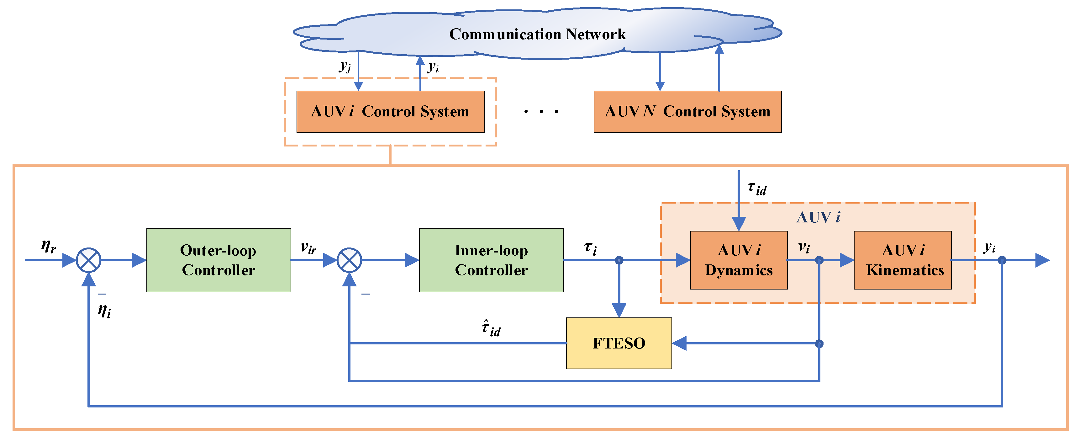
This section develops the FTESO-based distributed dual closed-loop model predictive control scheme for the AUV formation to perform trajectory tracking. A novel FTESO is designed to compensate the compound disturbances. Based on the model information reconstructed by FTESO, the DMPC optimization problems are formulated for the outer and inner loops under constraints such as actuator saturation and collision avoidance, respectively. The Laguerre function is applied to alleviate the computational load. The block diagram of proposed control scheme is depicted in Figure 2.

3.1. FTESO Design and Convergence Analysis

The AUV model is fundamental to controller design, but obtaining an accurate model in practice is challenging. Considering the superiority and effectiveness of the ESO technique in estimating and compensating for synthetic uncertainty, a novel fast FTESO is designed to simultaneously reconstruct the external disturbance and model uncertainties of multiple AUVs.

First, define the auxiliary velocity variable as ${\omega }_i\left(v_i\right)=M_i^{\ast }{v}_i+{\displaystyle \int v_i}$, the derivative of ${\omega }_i\left(v_i\right)$ with respect to time can be obtained from (4)

$${\omega }_i\left(v_i\right)=v_i-C_i^{\ast }\left(v_i\right)v_i-D_i^{\ast }\left(v_i\right)v_i-g_i^{\ast }\left({\eta }_i\right)+{\tau }_i+{\tau }_{id}.$$

(5)

For simplicity, denote $G_i\left({\eta }_i,v_i\right)=v_i-C_i^{\ast }\left(v_i\right)v_i-D_i^{\ast }\left(v_i\right)v_i-g_i^{\ast }\left({\eta }_i\right)$. Then, a new variable is defined as $z_{i1}={\omega }_i\left(v_i\right)$, and the order of the system is extended by additional state variables, $z_{i2}$ and $z_{i3}$, defined as $z_{i2}={\tau }_{id}$ and $z_{i3}={\dot{z}}_{i2}$ with ${\dot{z}}_{i3}={\sigma }_i$. It should be noted that the compound disturbances $z_{i2}$ are assumed to be bounded and continuously differentiable, and the components of its second derivative satisfies $\left|{\sigma }_{ip}\right|\le {\overline{\sigma }}_i$, $p=1,2,\dots ,5$. where ${\overline{\sigma }}_i$ is an unknown positive constant. Afterward, the dynamic model of the ith AUV can be extended as follows:

$$\left\{\begin{array}{l}{\dot{z}}_{i1}=G_i\left({\eta }_i,v_i\right)+{\tau }_i+z_{i2}\hfill \\ {\dot{z}}_{i2}=z_{i3}\hfill \\ {\dot{z}}_{i3}={\sigma }_i.\hfill \end{array}\right.$$

(6)

Denote ${\widehat{z}}_{i1}$, ${\widehat{z}}_{i2}$, and ${\widehat{z}}_{i3}$ as the observation values of states $z_{i1}$, $z_{i2}$, and $z_{i3}$ in the above extended system, and $e_{i1}={\widehat{z}}_{i1}-z_{i1}$, $e_{i2}={\widehat{z}}_{i2}-z_{i2}$, and $e_{i3}={\widehat{z}}_{i3}-z_{i3}$ as the observation errors of the velocity, the compound disturbances, and its first derivatives, respectively. Then, a third-order fast FTESO is proposed as follows:

$$\left\{\begin{array}{l}{\dot{\widehat{z}}}_{i1}={\widehat{z}}_{i2}-{\beta }_{i1}\left(si{g}^{{\alpha }_{i1}}\left(e_{i1}\right)+e_{i1}\right)+G_i\left({\eta }_i,v_i\right)+{\tau }_i\hfill \\ {\dot{\widehat{z}}}_{i2}={\widehat{z}}_{i3}-{\beta }_{i2}\left(si{g}^{{\alpha }_{i2}}\left(e_{i1}\right)+2si{g}^{{\alpha }_{i1}}\left(e_{i1}\right)+e_{i1}\right)\hfill \\ {\dot{\widehat{z}}}_{i3}=-{\beta }_{i3}\left(si{g}^{{\alpha }_{i3}}\left(e_{i1}\right)+2si{g}^{{\alpha }_{i2}}\left(e_{i1}\right)+si{g}^{{\alpha }_{i1}}\left(e_{i1}\right)\right)\hfill \end{array}\right.$$

(7)

where the observer gains satisfy ${\beta }_{ik}>0,k=1,2,3$, ${\alpha }_{i1}\in \left(2/3,1\right)$ and ${\alpha }_{i2}=2{\alpha }_{i1}-1$, and ${\alpha }_{i3}=3{\alpha }_{i1}-2$. Although the actual value of $z_{ik}$ is probably unavailable, its observed value ${\widehat{z}}_{ik}$ can be obtained by the above FTESO. The analysis and proof that ${\widehat{z}}_{ik}$ tracks the actual value are described below.

According to the extended system (6) and the proposed FTESO (7), we can obtain the observation error dynamics as follows:

$$\left\{\begin{array}{l}{\dot{e}}_{i1}=-{\beta }_{i1}\left(si{g}^{{\alpha }_{i1}}\left(e_{i1}\right)+e_{i1}\right)+e_{i2}\hfill \\ {\dot{e}}_{i2}=-{\beta }_{i2}\left(si{g}^{{\alpha }_{i2}}\left(e_{i1}\right)+2si{g}^{{\alpha }_{i1}}\left(e_{i1}\right)+e_{i1}\right)+e_{i3}\hfill \\ {\dot{e}}_{i3}=-{\beta }_{i3}\left(si{g}^{{\alpha }_{i3}}\left(e_{i1}\right)+2si{g}^{{\alpha }_{i2}}\left(e_{i1}\right)+si{g}^{{\alpha }_{i1}}\left(e_{i1}\right)\right)-{\sigma }_i.\hfill \end{array}\right.$$

(8)

The stability and convergence of the proposed FTESO are stated in the following theorem:

Theorem 1. 

Consider the AUV formation control system with the dynamic model (4) under Assumption 1. If the FTESO is proposed in the form of (9), with appropriate observer gains satisfying the prescribed constraints, then the observation errors $e_i={\left[e_{i1}^T,e_{i2}^T,e_{i3}^T\right]}^T$ will converge to the small region ${\mathsf{\Omega }}_i$ in finite time $T_{if}$. This implies that the error dynamics system (8) is finite-time uniformly ultimately bounded stable.

Proof of Theorem 1. 

Consider a Lyapunov candidate function as $V_{i1}\left(e\right)={\epsilon }_i^T{P}_i{\epsilon }_i$, where $P_i$ is a positive definite symmetric matrix and ${\epsilon }_i^T=\left[{\left(si{g}^{{\alpha }_{i1}}\left(e_{i1}\right)+e_{i1}\right)}^T,e_{i2}^T,e_{i3}^T\right]$ is introduced as an auxiliary error variable. It should be noted that $e_{i1}$, $e_{i2}$, and $e_{i3}$ will converge to origin in finite time, if the new state ${\epsilon }_i$ is finite-time stable. The time derivative of ${\epsilon }_i$, invoking (8), yields:

$$\begin{array}{l}{\dot{\epsilon }}_i=\left[\begin{array}{c}{\alpha }_{i1}{\left|e_{i1}\right|}^{{\alpha }_{i1}-1}{\dot{e}}_{i1}+{\dot{e}}_{i1}\\ {\dot{e}}_{i2}\\ {\dot{e}}_{i3}\end{array}\right]=\left[\begin{array}{c}{\alpha }_{i1}{\left|e_{i1}\right|}^{{\alpha }_{i1}-1}\left(e_{i2}-{\beta }_{i1}\left(si{g}^{{\alpha }_{i1}}\left(e_{i1}\right)+e_{i1}\right)\right)\\ \frac{e_{i3}}{2}-{\beta }_{i2}\left(si{g}^{{\alpha }_{i2}}\left(e_{i1}\right)+si{g}^{{\alpha }_{i1}}\left(e_{i1}\right)\right)\\ -{\beta }_{i3}\left(si{g}^{{\alpha }_{i3}}\left(e_{i1}\right)+si{g}^{{\alpha }_{i2}}\left(e_{i1}\right)\right)\end{array}\right]\\ +\left[\begin{array}{c}{e}_{i2}-{\beta }_{i1}\left(si{g}^{{\alpha }_{i1}}\left(e_{i1}\right)+e_{i1}\right)\\ \frac{e_{i3}}{2}-{\beta }_{i2}\left(si{g}^{{\alpha }_{i1}}\left(e_{i1}\right)+e_{i1}\right)\\ -{\beta }_{i3}\left(si{g}^{{\alpha }_{i2}}\left(e_{i1}\right)+si{g}^{{\alpha }_{i1}}\left(e_{i1}\right)\right)\end{array}\right]+\left[\begin{array}{c}{0}_5\\ 0_5\\ -{\sigma }_i\end{array}\right]=\mathit{diag}\left(\left[{\left|e_{i1}\right|}^{{\alpha }_{i1}-1},{\left|e_{i1}\right|}^{{\alpha }_{i1}-1},{\left|e_{i1}\right|}^{{\alpha }_{i1}-1}\right]\right)A_{i1}{\epsilon }_i+A_{i2}{\epsilon }_i+{\Phi }_i\end{array}$$

(9)

where ${\Phi }_i={\left[\begin{array}{ccc}{0}_5& 0_5& -{\sigma }_i\end{array}\right]}^T$ and the coefficient matrices $A_{i1}$ and $A_{i2}$ are expressed as:

$$A_{i1}=\left(\begin{array}{ccc}-{\alpha }_{i1}{\beta }_{i1}{I}_5& {\alpha }_{i1}{I}_5& 0_5\\ -{\beta }_{i2}{I}_5& 0_5& {\overline{e}}_i^{-1}{I}_5/2\\ -{\beta }_{i3}{\overline{e}}_i{I}_5& 0_5& 0_5\end{array}\right),\hspace{0.17em}{A}_{2i}=\left(\begin{array}{ccc}-{\beta }_{i1}{I}_5& I_5& 0_5\\ -{\beta }_{i2}{I}_5& 0_5& I_5/2\\ -{\beta }_{i3}{\overline{e}}_i{I}_5& 0_5& 0_5\end{array}\right)$$

(10)

with ${\overline{e}}_i={\left|e_{i1}\right|}^{{\alpha }_{i1}-1}$. From the characteristic polynomials of $A_{i1}$ and $A_{i2}$ that all their eigenvalues have negative real parts if the observer gains are set as ${\beta }_{ik}>0$, indicating that $A_{i1}$ and $A_{i2}$ are Hurwitz matrices. Thus, symmetric and positive definite matrices $Q_{i1}$ and $Q_{i2}$ exist that satisfy the following Lyapunov equations:

$$\left\{\begin{array}{c}{A}_{i1}^T{P}_i+P_i{A}_{i1}=-Q_{i1}\\ A_{i2}^T{P}_i+P_i{A}_{i2}=-Q_{i2}.\end{array}\right.$$

(11)

Differentiating $V_{i1}\left(e\right)$ with respect to time yields the following:

$$\begin{array}{ll}{\dot{V}}_{i1}& ={\epsilon }_i^T\left[\mathit{diag}\left(\left[{\overline{e}}_i,{\overline{e}}_i,{\overline{e}}_i\right]\right)\left(A_{i1}^T{P}_i+P_i{A}_{i1}\right)\right]{\epsilon }_i+{\epsilon }_i^T\left(A_{i2}^T{P}_i+P_i{A}_{i2}\right){\epsilon }_i+2{\epsilon }_i^T{P}_i{\Phi }_i\\ & =-{\epsilon }_i^T\left[\mathit{diag}\left(\left[{\overline{e}}_i,{\overline{e}}_i,{\overline{e}}_i\right]\right)Q_{i1}\right]{\epsilon }_i-{\epsilon }_i^T{Q}_{i2}{\epsilon }_i+2{\epsilon }_i^T{P}_i{\Phi }_i\le -{\overline{e}}_i^{\max }{\epsilon }_i^T{Q}_{i1}{\epsilon }_i-{\epsilon }_i^T{Q}_{i2}{\epsilon }_i+2‖{\epsilon }_i‖‖P_i‖‖{\Phi }_i‖\end{array}$$

(12)

where ${\overline{e}}_i^{\max }={\left|e_{i1}\right|}_{\max }^{{\alpha }_{i1}-1}$ and ${\left|e_{i1}\right|}_{\max }=\max \left\{\left|e_{i11}\right|,\dots ,\left|e_{i15}\right|\right\}$. Given the fact that ${\left|e_{i1}\right|}_{\max }\le ‖e_{i1}‖\le {‖{\epsilon }_i‖}^{1/{\alpha }_{i1}}$ and ${\alpha }_{i1}\in \left(\frac{2}{3},1\right)$, we can obtain the following:

$$\begin{array}{ll}{\dot{V}}_{i1}& \le -{‖{\epsilon }_i‖}^{\frac{{\alpha }_{i1}-1}{{\alpha }_{i1}}}{\epsilon }_i^T{Q}_{i1}{\epsilon }_i-{\epsilon }_i^T{Q}_{i2}{\epsilon }_i+2‖{\epsilon }_i‖‖P_i‖‖{\Phi }_i‖\\ & \le -{\lambda }_{\min }\left(Q_{i1}\right){‖{\epsilon }_i‖}^{3-\frac{1}{{\alpha }_{i1}}}-{\lambda }_{\min }\left(Q_{i2}\right){‖{\epsilon }_i‖}^2+2‖{\epsilon }_i‖‖P_i‖‖{\Phi }_i‖.\end{array}$$

(13)

Since ${\sigma }_i$ is assumed to be bounded reasonably by $\left|{\sigma }_{ip}\right|\le {\overline{\sigma }}_i$, we have $2‖{\epsilon }_i‖‖P_i‖‖{\Phi }_i‖\le 2\sqrt{5}{\overline{\sigma }}_i‖{\epsilon }_i‖‖P_i‖\le 2\sqrt{5}{\overline{\sigma }}_i{\lambda }_{\min }{\left(P_i\right)}^{-\frac{1}{2}}{V}_{i1}^{\frac{1}{2}}‖P_i‖$, by using the inequality

$${\lambda }_{\min }\left(P_i\right){‖{\epsilon }_i‖}^2\le V_{i1}\le {\lambda }_{\max }\left(P_i\right){‖{\epsilon }_i‖}^2$$

(14)

Then, inequality (13) becomes the following:

$$\begin{array}{ll}{\dot{V}}_{i1}& \le -{\lambda }_{\min }\left(Q_{i1}\right){\lambda }_{\max }{\left(P_i\right)}^{\frac{1}{2{\alpha }_{i1}}-\frac{3}{2}}{V}_{1i}^{{}^{\frac{3}{2}-\frac{1}{2{\alpha }_{i1}}}}-{\lambda }_{\min }\left(Q_{i2}\right){\lambda }_{\max }{\left(P_i\right)}^{-1}{V}_{i1}+2\sqrt{5}{\overline{\sigma }}_i‖P_i‖{\lambda }_{\min }{\left(P_i\right)}^{-\frac{1}{2}}{V}_{i1}^{\frac{1}{2}}\\ & \le -{\lambda }_{i1}{V}_{i1}^{{}^{\frac{3}{2}-\frac{1}{2{\alpha }_{i1}}}}-{\lambda }_{i2}{V}_{i1}+{\lambda }_{i3}{V}_{i1}^{{}^{\frac{1}{2}}}\end{array}$$

(15)

where ${\lambda }_{i1}=-{\lambda }_{\min }\left(Q_{i1}\right){\lambda }_{\max }{\left(P_i\right)}^{\frac{1}{2{\alpha }_{i1}}-\frac{3}{2}}$, ${\lambda }_{i2}=-{\lambda }_{\min }\left(Q_{i2}\right){\lambda }_{\max }{\left(P_i\right)}^{-1}$, and ${\lambda }_{i3}=2\sqrt{5}{\overline{\sigma }}_i‖P_i‖{\lambda }_{\min }{\left(P_i\right)}^{-\frac{1}{2}}$.

It can be seen that (15) has the same form as the sufficient condition in Lemma 1 2. Thus, the error trajectories of the proposed FTESO (7) are fast finite-time uniformly ultimately bounded stable. The state observation errors $e_i$ will converge to a small region ${\mathsf{\Omega }}_i$ in the finite time $T_{if}$. Moreover, the settling time $T_{if}$ is subject to the constraint:

$$T_{if}\le \frac{\ln \left(\left({\lambda }_{i2}-{\overline{\lambda }}_{i2}\right)V_{i1}{\left(e_0\right)}^{\frac{1}{2{\alpha }_{i1}}-\frac{1}{2}}/\left({\lambda }_{i1}-{\overline{\lambda }}_{i1}\right)+1\right)}{\left({\lambda }_{i2}-{\overline{\lambda }}_{i2}\right)\left(\frac{1}{2{\alpha }_{i1}}-\frac{1}{2}\right)}.$$

(16)

And the stable region ${\mathsf{\Omega }}_i$ is denoted as

$${\mathsf{\Omega }}_i=\left\{\left.e\right|{\overline{\lambda }}_{i1}{V}_{i1}{\left(e\right)}^{1-\frac{1}{2{\alpha }_{i1}}}+{\overline{\lambda }}_{i2}{V}_{i1}{\left(e\right)}^{\frac{1}{2}}<{\lambda }_{i3}\right\}$$

(17)

where ${\overline{\lambda }}_{i1}$ and ${\overline{\lambda }}_{i2}$ are arbitrary constants that meet the conditions ${\overline{\lambda }}_{i1}\in \left(0,{\lambda }_{i1}\right)$ and ${\overline{\lambda }}_{i2}\in \left(0,{\lambda }_{i2}\right)$. This completes the proof. □

Remark 1. 

Contrasting our proposed FTESO (7) with the FTESO in [37], our approach factors in the dynamics of disturbances and uncertainties to achieve a higher degree of estimation accuracy. Our usage of fractional powers within the FTESO allows for a quick finite-time convergence. It can be noted that the size of the attraction region ${\mathsf{\Omega }}_i$ hinges upon the selection of the observer gains ${\beta }_{ik}$ and ${\alpha }_{i1}$. By increasing ${\beta }_{ik}$ or decreasing ${\alpha }_{i1}$, the attraction region of the observation error system can be expanded and the convergence speed can be improved, but excessive tuning will lead to undesired overshoot and oscillation. As a result, a trade-off should be taken for ${\beta }_{ik}$ and ${\alpha }_{i1}$.

3.2. Outer-Loop Formation Prediction Control Law

In this subsection, we design a DMPC-based outer-loop formation controller. This controller, which draws on the information interaction with neighbors, facilitates the positional tracking of the ith AUV. The controller operates under composite constraints and ensures the avoidance of collisions. Then, we formulate a constrained QP problem in accordance with the control objective to obtain the optimal driving speed.

To facilitate the recursive model prediction and the implementation of the control law, the kinematic model (1) is discretized by using the Forward-Euler method with a sampling period $T_s$, resulting in following discrete model:

$${\eta }_i\left(k+1\right)={\eta }_i\left(k\right)+J_i\left(k\right)v_i\left(k\right)T_s.$$

(18)

To smoothen the speed change of the AUV, the velocity increment $\Delta u_{iv}\left(k\right)=v_i\left(k\right)-v_i\left(k-1\right)$ is taken as the control input. $x_{i\eta }\left(k\right)={\left[\begin{array}{cc}{\eta }_i\left(k\right)& v_i\left(k-1\right)\end{array}\right]}^T$ is denoted as the state variable of the prediction model. The augmented state-space model of the outer-loop subsystem can be derived as:

$$x_{i\eta }\left(k+1\right)=A_{i\eta }{x}_{i\eta }\left(k\right)+B_{i\eta }\Delta u_{iv}\left(k\right)$$

(19)

$$y_{i\eta }\left(k\right)=C_{i\eta }{x}_{i\eta }\left(k\right)$$

(20)

where $A_{i\eta }=\left[\begin{array}{cc}{I}_5& J_i\left(k\right)T_s\\ 0_5& I_5\end{array}\right]\in {ℝ}^{10\times 10}$, $B_{i\eta }=\left[\begin{array}{c}{J}_i\left(k\right)T_s\\ I_5\end{array}\right]\in {ℝ}^{10\times 5}$, and $C_{i\eta }=\left[\begin{array}{cc}{I}_5& 0_5\end{array}\right]\in {ℝ}^{5\times 10}$.

According to the state prediction model (19) and (20), we can calculate the predicted state sequence of the system when given an input sequence. Let $N_{p1}$ and $N_{c1}$ denote the prediction and control horizon of the outer-loop controller, respectively. The predicted state sequence and the input incremental sequence are usually represented by compact vectors:

$$Y_{i\eta }=\left[\begin{array}{c}{y}_{i\eta }\left(k+1|k\right)\\ y_{i\eta }\left(k+2|k\right)\\ ⋮\\ y_{i\eta }\left(k+N_{p1}|k\right)\end{array}\right]\in {ℝ}^{5N_{p1}},x_{i\eta }=\left[\begin{array}{c}{x}_{i\eta }\left(k+1|k\right)\\ x_{i\eta }\left(k+2|k\right)\\ ⋮\\ x_{i\eta }\left(k+N_{p1}|k\right)\end{array}\right]\in {ℝ}^{10N_{p1}}$$

(21)

$$\Delta U_{iv}=\left[\begin{array}{c}\Delta u_{iv}\left(k|k\right)\\ \Delta u_{iv}\left(k+1|k\right)\\ ⋮\\ \Delta u_{iv}\left(k+N_{c1}-1|k\right)\end{array}\right]\in {ℝ}^{5N_{c1}}$$

(22)

where $y_{i\eta }\left(k+l|k\right)$ and $x_{i\eta }\left(k+l|k\right)$ are the output vector $y_{i\eta }\left(k+l\right)$ and state vector $x_{i\eta }\left(k+l\right)$ predicted at time k, respectively. $\Delta u_{iv}\left(k+j|k\right)$ denotes the input increment $\Delta u_{iv}\left(k+j\right)$ predicted at the same time k. Then, we characterize the relationship between the predicted output vector sequence and the control increment sequence through the following prediction equation based on the recurrence relations:

$$Y_{i\eta }=H_{ix}^1{x}_{i\eta }\left(k\right)+H_{iu}^1\Delta U_{iv}$$

(23)

where $x_{i\eta }\left(k\right)$ is the initial state, $H_{ix}^1={\left[C_{i\eta }{A}_{i\eta },C_{i\eta }{A}_{i\eta }^2,\dots ,C_{i\eta }{A}_{i\eta }^{N_{p1}}\right]}^T\in {ℝ}^{5N_{p1}\times 10}$ and

$H_{iu}^1=\left[\begin{array}{cccc}{C}_{i\eta }{B}_{i\eta }& 0_5& \cdots & 0_5\\ C_{i\eta }{A}_{i\eta }{B}_{i\eta }& C_{i\eta }{B}_{i\eta }& \cdots & 0_5\\ ⋮& ⋮& \ddots & ⋮\\ C_{i\eta }{A}_{i\eta }^{N_{p1}-1}{B}_{i\eta }& C_{i\eta }{A}_{i\eta }^{N_{p1}-2}{B}_{i\eta }& \cdots & C_{i\eta }{A}_{i\eta }^{N_{p1}-N_{c1}}{B}_{i\eta }\end{array}\right]\in {ℝ}^{5N_{p1}\times 5N_{c1}}$.

Considering the control objective, the constraints within the outer-loop subsystem are considered. First, we set upper and lower boundaries for the amplitude of the control input $u_{iv}\left(k\right)$ and the input increment $\Delta u_{iv}\left(k\right)$:

$$u_{iv}^{\min }\le u_{iv}\left(k\right)\le u_{iv}^{\max }$$

(24)

$$\Delta u_{iv}^{\min }\le \Delta u_{iv}\left(k\right)\le \Delta u_{iv}^{\max }$$

(25)

where $u_{iv}^{\min }$ and $\Delta u_{iv}^{\min }$ represent the predefined lower bounds, and $u_{iv}^{\max }$ and $\Delta u_{iv}^{\max }$ represent the predefined upper bounds.

Next, to assure safe navigation throughout the formation construction stage, we need to consider the collision avoidance constraints between AUVs. The primitive collision avoidance constraints of the ith AUV can be transformed into a convex constraint, as follows:

$$‖S\left(y_{i\eta }\left(k+l|k\right)-y_{j\eta }\left(k+l|k\right)\right)‖\ge r_s,\hspace{0.33em}j\in {\Xi }_i$$

(26)

where $l=1,2,\dots ,N_{p1}$ and $r_s$ is the preset minimum allowable distance between the ith AUV and the jth AUV. $S$ denotes a scaling matrix. Let $r_d$ be the radius of the safe detection zone for the ith AUV. ${\Xi }_i$ is the set of those AUVs that contain within $r_d$. Let the nominal value ${\overline{y}}_{i\eta }$ represent an initial guess of the actual value $y_{i\eta }$ for convexifying the collision avoidance constraint. It follows from (26) that a sufficient condition for upholding the collision avoidance constraint is the following:

$${\overline{d}}_{ij}^T\left(k+l|k\right)S^{T}S\left(y_{i\eta }\left(k+l|k\right)-{\overline{y}}_{j\eta }\left(k+l|k\right)\right)\ge r_s‖S{\overline{d}}_{ij}\left(k+l|k\right)‖$$

(27)

where ${\overline{d}}_{ij}\left(k+l|k\right)={\overline{y}}_{i\eta }\left(k+l|k\right)-{\overline{y}}_{j\eta }\left(k+l|k\right)$. In order to express the constraints in a compact matrix form, define ${\overline{R}}_l=r_s‖S{\overline{d}}_{ij}\left(k+l|k\right)‖+{\overline{d}}_{ij}^T\left(k+l|k\right)S^{T}S{\overline{y}}_{j\eta }\left(k+l|k\right)$, ${\overline{R}}_{ij}={\left[{\overline{R}}_1,{\overline{R}}_2,\dots ,{\overline{R}}_{N_{p1}}\right]}^T$ and ${\overline{S}}_{ij}=\mathit{diag}\left\{{\overline{S}}_1,{\overline{S}}_2,\dots ,{\overline{S}}_{N_{p1}}\right\}$, and ${\overline{S}}_l={\overline{d}}_{ij}^T\left(k+l|k\right)S^{T}S$. Then, (27) can be rewritten as ${\overline{S}}_{ij}{Y}_{i\eta }\ge {\overline{R}}_{ij}$. Substitute (23) to derive the collision avoidance constraint as follows:

$${\overline{S}}_{ij}{H}_{iu}^1\Delta U_{iv}\ge {\overline{R}}_{ij}-{\overline{S}}_{ij}{H}_{ix}^1{x}_{i\eta }\left(k\right).$$

(28)

The input amplitude constraint (24) can be converted to the input incremental constraint, associating (25) and (28), expressed in the compact linear constraint form as follows:

$${\Gamma }_{i\eta }\Delta U_{iv}\le {\mathsf{\gamma }}_{i\eta }$$

(29)

where ${\Gamma }_{i\eta }=\left[\begin{array}{c}{I}_{5N_{c1}}\\ -I_{5N_{c1}}\\ I_{\eta 1}\\ -I_{\eta 1}\\ -{\overline{S}}_{ij}{H}_{iu}^1\end{array}\right]$, ${\mathsf{\gamma }}_{i\eta }=\left[\begin{array}{c}\Delta U_{iv}^{\max }\\ -\Delta U_{iv}^{\min }\\ U_{iv}^{\max }-I_{\eta 2}{u}_i\left(k-1\right)\\ -U_{iv}^{\min }+I_{\eta 2}{u}_i\left(k-1\right)\\ {\overline{S}}_{ij}{H}_{ix}^1{x}_{i\eta }\left(k\right)-{\overline{R}}_{ij}\end{array}\right]$, $I_{\eta 1}=\left[\begin{array}{cccc}{I}_5& 0_5& \cdots & 0_5\\ I_5& I_5& \cdots & 0_5\\ ⋮& ⋮& \ddots & ⋮\\ I_5& I_5& \cdots & I_5\end{array}\right]\in {ℝ}^{5N_{c1}\times 5N_{c1}}$, and $I_{\eta 2}={\left[I_5,I_5,\dots ,I_5\right]}^T\in {ℝ}^{5N_{c1}}$.

In order to achieve the control objective of formation positional tracking with low energy requirements, we define the local distributed cost function in the outer-loop subsystem of the ith AUV in a discretized form:

$$\begin{array}{ll}{J}_{i\eta }\left(k\right)=& {\displaystyle \sum _{l=1}^{N_{p1}}{‖\left(y_{i\eta }\left(k+\left.l\right|k\right)-y_{if}\left(k+l\right)\right)‖}_{Q_{if}}^2}+{\displaystyle \sum _{l=0}^{N_{c1}-1}{‖\Delta u_{iv}\left(k+\left.l\right|k\right)‖}_{R_{i1}}^2}\\ & +{\displaystyle \sum _{l=1}^{N_{p1}}{\displaystyle \sum _{j\in {\mathrm{N}}_i}{a}_{ij}}}{‖\left(y_{i\eta }\left(k+\left.l\right|k\right)-y_{ij}\left(k+l\right)\right)‖}_{Q_{ij}}^2\end{array}$$

(30)

where $Q_{if}$, $Q_{ij}$, and $R_{i1}$ are the weight matrices. $y_{if}\left(k+l\right)={\eta }_r\left(k+l\right)+r_{if}\left(k+l\right)$ with $r_{if}\left(k+l\right)$ represents the formation configuration. $y_{ij}\left(k+l\right)=y_{j\eta }\left(k+l\right)+r_{ij}\left(k+l\right)$ with $r_{ij}\left(k+l\right)$ represents the predefined relative distance between the ith AUV and its neighbor jth AUV. $N_{p1}$ indicates the degree of prediction of future tracking errors. The larger it is, the better the tracking accuracy and stability. The smaller $N_{c1}$ is, the worse the dynamic response is, and conversely the more maneuverable the control is. $Q_{if}$ is the position tracking matrix, the larger it is, the better the tracking accuracy and dynamic response. $Q_{ij}$ is the relative position matrix, the larger it is, the better the ability of the formation to maintain the preset configuration. $R_{i1}$ is the control increment weight matrix, mainly to limit the drastic change of $\Delta u_{iv}$.

Based on the above derivations, we can formulate the optimization problem for the outer-loop subsystem of the ith AUV at the sampling instant k within the receding-horizon framework:

$$\begin{array}{l}\underset{\Delta U_{iv}}{\min }\hspace{0.17em}{J}_{i\eta }\left(k\right)\\ s.t.\hspace{0.33em}{\Gamma }_{i\eta }\Delta U_{iv}\le {\mathsf{\gamma }}_{i\eta }.\end{array}$$

(31)

To simplify the computation of (31), it can be transformed into a convex QP problem. This problem is solved over a finite receding horizon using a QP solver. The standard convex QP form of the DMPC problem (31) can be derived:

$$\begin{array}{l}\Delta U_{iv}^{\ast }=\underset{\Delta U_{iv}}{\arg \min }\left(\frac{1}{2}\Delta U_{iv}^T{W}_{i\eta }\Delta U_{iv}+f_{i\eta }^T\Delta U_{iv}\right)\\ s.t.\hspace{0.33em}{\Gamma }_{i\eta }\Delta U_{iv}\le {\mathsf{\gamma }}_{i\eta }\end{array}$$

(32)

where $W_{i\eta }={\overline{R}}_{i1}+H_{iu}^{1T}{\overline{Q}}_{if}{H}_{iu}^1+{\displaystyle {\sum }_{j\in {\mathrm{N}}_i}{a}_{ij}{H}_{iu}^{1T}{\overline{Q}}_{ij}{H}_{iu}^1}$,

$f_{i\eta }=H_{iu}^{1T}{\overline{Q}}_{if}\left(H_{ix}^1{x}_{i\eta }^{}-Y_{if}\right)+{\displaystyle {\sum }_{j\in {\mathrm{N}}_i}{a}_{ij}{H}_{iu}^{1T}{\overline{Q}}_{ij}\left(H_{ix}^1{x}_{i\eta }^{}-Y_{ij}\right)}$, with $Y_{if}={\left[y_{if}\left(k+1\right),\dots ,y_{if}\left(k+N_{p1}\right)\right]}^T$, $Y_{ij}={\left[y_{ij}\left(k+1\right),\dots ,y_{ij}\left(k+N_{p1}\right)\right]}^T$, ${\overline{Q}}_{if}=\mathit{diag}\left\{Q_{if},Q_{if},\dots ,Q_{if}\right\}\in {ℝ}^{5N_{p1}\times 5N_{p1}}$, ${\overline{Q}}_{ij}$, and ${\overline{R}}_{i1}$ are similar to ${\overline{Q}}_{if}$, both corresponding compact matrices.

By solving the QP optimization problem in (32) online, we obtain the optimal control input increment sequence $\Delta U_{iv}^{\ast }$. Of this sequence, we only utilize the first element $\Delta u_{iv}^{\ast }\left(k|k\right)$ for receding optimization. Once $\Delta u_{iv}^{\ast }\left(k\right)$ is determined, we obtain $v_i\left(k\right)$ which serves as the desired driving speed for the inner-loop controller of the ith AUV, i.e.,

$$v_{ir}\left(k\right)=v_i\left(k\right)=v_i\left(k-1\right)+\Delta u_{iv}^{\ast }\left(k\right).$$

(33)

3.3. Inner-Loop Formation Prediction Control Law

In this subsection, with the aid of the proposed FTESO, we design a DMPC-based formation controller for the inner-loop subsystem to obtain the optimal driving force and moment for the ith AUV to track the desired speed.

The dynamic model (4) is discretized with a sampling period $T_s$, yielding the following discretized model:

$$v_i\left(k+1\right)=\left(I-M_i^{\ast }{}^{-1}{T}_s\left(C_i^{\ast }+D_i^{\ast }\right)\right)v_i\left(k\right)+M_i^{\ast }{}^{-1}{T}_s{\tau }_i\left(k\right)+M_i^{\ast }{}^{-1}{T}_s{\widehat{\tau }}_{id}\left(k\right)$$

(34)

where ${\widehat{\tau }}_{id}$ represents the compound disturbance compensated by FTESO (7), which is supposed to be invariant over a short period. It should be noted that we assume the center of gravity and buoyancy of the ith AUV to coincide, which allows $g_i\left({\eta }_i\right)$ to approximate to zero. We select $x_{iv}\left(k\right)={\left[\begin{array}{cc}{v}_i\left(k\right)& {\tau }_i\left(k-1\right)\end{array}\right]}^T$ as the state variable and take the increment $\Delta u_{i\tau }\left(k\right)={\tau }_i\left(k\right)-{\tau }_i\left(k-1\right)$ as the control input. This allows us to reformulate the inner-loop predictive model as follows:

$$x_{iv}\left(k+1\right)=A_{iv}{x}_{iv}\left(k\right)+B_{iv}\Delta u_{i\tau }\left(k\right)+D_{iv}$$

(35)

$$y_{iv}\left(k\right)=C_{iv}{x}_{iv}\left(k\right)$$

(36)

where $A_{iv}=\left[\begin{array}{cc}{I}_5-M_i^{\ast }{}^{-1}{T}_s\left(C_i^{\ast }+D_i^{\ast }\right)& M_i^{\ast }{}^{-1}{T}_s\\ 0_5& I_5\end{array}\right]\in {ℝ}^{10\times 10}$, $B_{iv}=\left[\begin{array}{c}{M}_i^{\ast }{}^{-1}{T}_s\\ I_5\end{array}\right]\in {ℝ}^{10\times 5}$, $C_{iv}=\left[\begin{array}{cc}{I}_5& 0_5\end{array}\right]\in {ℝ}^{5\times 10}$, and $D_{iv}=\left[\begin{array}{c}{M}_i^{\ast }{}^{-1}{T}_s{\widehat{\tau }}_{id}\\ 0_{5\times 1}\end{array}\right]\in {ℝ}^{10}$. Similar to our previous approach, we can characterize the relationship between the predicted output vector sequence and the control increment sequence using the following prediction equation:

$$Y_{iv}=H_{ix}^2{x}_{iv}\left(k\right)+H_{iu}^2\Delta U_{i\tau }+{\overline{D}}_{iv}$$

(37)

where $Y_{iv}={\left[y_{iv}\left(k+1|k\right),y_{iv}\left(k+2|k\right),\dots ,y_{iv}\left(k+N_{p2}|k\right)\right]}^T\in {ℝ}^{5N_{p2}}$,

$\Delta U_{i\tau }={\left[\Delta u_{i\tau }\left(k|k\right),\Delta u_{i\tau }\left(k+1|k\right),\dots ,\Delta u_{i\tau }\left(k+N_{c2}-1|k\right)\right]}^T\in {ℝ}^{5N_{c2}}$,

$H_{ix}^2={\left[C_{iv}{A}_{iv},C_{iv}{A}_{iv}^2,\dots ,C_{iv}{A}_{iv}^{N_{p2}}\right]}^T\in {ℝ}^{5N_{p2}\times 10}$,

$H_{iu}^2=\left[\begin{array}{cccc}{C}_{iv}{B}_{iv}& 0_5& \cdots & 0_5\\ C_{iv}{A}_{iv}{B}_{iv}& C_{iv}{B}_{iv}& \cdots & 0_5\\ ⋮& ⋮& \ddots & ⋮\\ C_{iv}{A}_{iv}^{N_{p2}-1}{B}_{iv}& C_{iv}{A}_{iv}^{N_{p2}-2}{B}_{iv}& \cdots & C_{iv}{A}_{iv}^{N_{p2}-N_{c2}}{B}_{iv}\end{array}\right]\in {ℝ}^{5N_{p2}\times 5N_{c2}}$, and

${\overline{D}}_{iv}={\left[C_{iv}{D}_{iv},C_{iv}{A}_{iv}{D}_{iv}+C_{iv}{D}_{iv},\dots ,C_{iv}{\displaystyle \sum _{n=0}^{N_{p2}-1}{A}_{iv}^n}{D}_{iv}\right]}^T\in {ℝ}^{5N_{p2}}$. $N_{p2}$ and $N_{c2}$ denote the prediction and control horizon of the inner-loop controller, respectively.

According to the control objective, we assess the constraints on the control input increment and the actuator saturation in the inner-loop subsystem, as follows:

$$\Delta u_{i\tau }^{\min }\le \Delta u_{i\tau }\left(k\right)\le \Delta u_{i\tau }^{\max }$$

(38)

$${\tau }_i^{\min }\le {\tau }_i\left(k\right)\le {\tau }_i^{\max }$$

(39)

where ${\tau }_i^{\min }$ and $\Delta u_{iv}^{\min }$ represent predefined lower bounds, while ${\tau }_i^{\max }$ and $\Delta u_{iv}^{\max }$ denote predefined upper bounds. The actuator saturation constraint (39) can be transformed into an input incremental constraint, and we can express the above constraints in a compact linear constraint form:

$${\Gamma }_{iv}\Delta U_{i\tau }\le {\mathsf{\gamma }}_{iv}$$

(40)

where ${\Gamma }_{iv}=\left[\begin{array}{c}{I}_{5N_{c2}}\\ -I_{5N_{c2}}\\ I_{v1}\\ -I_{v1}\end{array}\right]$, ${\mathsf{\gamma }}_{i\eta }=\left[\begin{array}{c}\Delta U_{i\tau }^{\max }\\ -\Delta U_{i\tau }^{\min }\\ {\overline{\tau }}_i^{\max }-I_{v2}{\tau }_i\left(k-1\right)\\ -{\overline{\tau }}_{iv}^{\min }+I_{v2}{\tau }_i\left(k-1\right)\end{array}\right]$, with $I_{v1}=\left[\begin{array}{cccc}{I}_5& 0_5& \cdots & 0_5\\ I_5& I_5& \cdots & 0_5\\ ⋮& ⋮& \ddots & ⋮\\ I_5& I_5& \cdots & I_5\end{array}\right]\in {ℝ}^{5N_{c2}\times 5N_{c2}}$ and $I_{v2}={\left[I_5,I_5,\dots ,I_5\right]}^T\in {ℝ}^{5N_{c2}}$.

To achieve the convergence of the formation tracking velocity to the desired value, we define the local distributed cost function of the inner-loop subsystem as follows:

$$J_{iv}\left(k\right)={\displaystyle \sum _{l=1}^{N_{p2}}{‖\left(y_{iv}\left(k+\left.l\right|k\right)-v_{ir}\left(k+l\right)\right)‖}_{Q_{iv}}^2}+{\displaystyle \sum _{l=0}^{N_{c2}-1}{‖\Delta u_{i\tau }\left(k+\left.l\right|k\right)‖}_{R_{i2}}^2}$$

(41)

where $y_{iv}\left(k+\left.l\right|k\right)$ and $\Delta u_{i\tau }\left(k+\left.j\right|k\right)$ denote the predicted value of $y_{iv}\left(k+l\right)$ and $\Delta u_{i\tau }\left(k+j\right)$ at time k, respectively. $Q_{iv}$ and $R_{i2}$ are given weight matrices.

By substituting (37) into (41), we can formulate the DMPC optimization problem for the inner-loop subsystem of the ith AUV at sampling instant k as the following QP form:

$$\begin{array}{l}\Delta U_{i\tau }^{\ast }=\underset{\Delta U_{i\tau }}{\arg \min }\left(\frac{1}{2}\Delta U_{i\tau }^T{W}_{iv}\Delta U_{i\tau }+f_{iv}^T\Delta U_{i\tau }\right)\\ s.t.\hspace{0.33em}{\Gamma }_{iv}\Delta U_{i\tau }\le {\mathsf{\gamma }}_{iv}\end{array}$$

(42)

where $W_{iv}={\overline{R}}_{i2}+H_{iu}^{2T}{\overline{Q}}_{iv}{H}_{iu}^2$ and $f_{iv}=H_{iu}^{2T}{\overline{Q}}_{iv}\left(H_{ix}^2{x}_{iv}+{\overline{D}}_{iv}-V_{ir}\right)$, with $v_{ir}={\left[v_{ir}\left(k+1\right),\dots ,v_{ir}\left(k+N_{p2}\right)\right]}^T\in {ℝ}^{5N_{p2}}$, ${\overline{Q}}_{iv}=\mathit{diag}\left\{Q_{iv},Q_{iv},\dots ,Q_{iv}\right\}\in {ℝ}^{5N_{p2}\times 5N_{p2}}$, and ${\overline{R}}_{i2}=\mathit{diag}\left\{R_{i2},R_{i2},\dots ,R_{i2}\right\}\in {ℝ}^{5N_{c2}\times 5N_{c2}}$.

The solution of the QP optimization problem (42) yields the optimal control input increment sequence $\Delta U_{i\tau }^{\ast }$ at time k. However, only the first element $\Delta u_{i\tau }^{\ast }\left(k|k\right)$ of the sequence is used for the ith AUV to obtain the optimal control force and moment ${\tau }_i^{\ast }\left(k\right)={\tau }_i\left(k-1\right)+\Delta u_{i\tau }^{\ast }\left(k\right)$. The $\Delta u_{i\tau }^{\ast }\left(k\right)$ is recalculated at each sampling instant, the ith AUV repeatedly calculates and executes ${\tau }_i^{\ast }\left(k\right)$ to achieve receding optimization. The predicted state $x_{iv}\left(k+1\right)$ and the optimal input ${\tau }_i^{\ast }\left(k\right)$ are both determined solely by the current state $x_{iv}\left(k\right)$.

With the parallel optimization of N AUV subsystems, all local optimization problems are solved simultaneously at each sampling moment. One or more information interactions occur between local controllers to obtain the optimal input sequence for that moment. Thus, the proposed control law can compensate well for the compound disturbances, which consist of model uncertainties and external disturbances. This occurs throughout the iterative optimization process, while simultaneously ensuring collision avoidance and formation tracking control tasks under complex constraints.

3.4. Use of Laguerre Functions in the DMPC Design

This subsection introduces a strategy to handle the computational burden caused by a longer control horizon and dual closed-loop structure. This is the main difficulty in our theoretical analysis. The Laguerre orthogonal functions are leveraged in the DMPC design to decrease the order of the input incremental matrices. This approach permits a reduction in input variables during each control cycle, thereby reducing the computational burden in the time interval and improving real-time performance.

The Laguerre functions are a set of discrete orthogonal polynomial functions, let it be $l_1\left(k\right),l_2\left(k\right),\dots ,l_M\left(k\right)$, the z-transfer of the mth Laguerre function is expressed as follows:

$${\mathrm{{\rm X}}}_m\left(z\right)=\frac{\sqrt{1-a^2}}{z-a}{\left[\frac{1-az}{z-a}\right]}^{m-1}$$

(43)

where $0\le a<1$ denotes the pole of the Laguerre function, also known as the scaling factor. It can be verified that ${\mathrm{{\rm X}}}_m$ satisfies the following orthogonality:

$$\left\{\begin{array}{l}\frac{1}{2\pi }{\displaystyle {\int }_{-\pi }^{\pi }{\mathrm{{\rm X}}}_m\left(e^{j\omega }\right){\mathrm{{\rm X}}}_n{\left(e^{j\omega }\right)}^{\ast }d\omega =1m=n}\hfill \\ \frac{1}{2\pi }{\displaystyle {\int }_{-\pi }^{\pi }{\mathrm{{\rm X}}}_m\left(e^{j\omega }\right){\mathrm{{\rm X}}}_n{\left(e^{j\omega }\right)}^{\ast }d\omega =0m\ne n}\hfill \end{array}\right.$$

(44)

where ${\left(·\right)}^{\ast }$ denotes complex conjugate of $\left(·\right)$.

The discrete Laguerre functions are defined by taking the inverse Z-transform of (43), i.e., $l_m\left(k\right)=Z^{-1}\left\{{\mathrm{{\rm X}}}_m\left(z\right)\right\}$. Given the network structure of ${\mathrm{{\rm X}}}_m\left(z\right)$ and the recurrence relation, the set of discrete Laguerre functions satisfies the following difference equation:

$$L\left(k+1\right)=\Xi L\left(k\right)$$

(45)

where $\Xi =\left[\begin{array}{ccccc}a& 0& 0& \cdots & 0\\ \beta & a& 0& \cdots & 0\\ -a\beta & \beta & a& \cdots & 0\\ ⋮& ⋮& ⋮& \ddots & ⋮\\ {\left(-a\right)}^{M-2}\beta & {\left(-a\right)}^{M-3}\beta & {\left(-a\right)}^{M-4}\beta & \cdots & a\end{array}\right]$ and $L\left(k\right)={\left[l_1\left(k\right),l_2\left(k\right),\dots ,l_M\left(k\right)\right]}^T$, with $\beta =1-a^2$ and initial condition $L\left(0\right)=\sqrt{\beta }{\left[1,-a,a^2,-a^3,\dots ,{\left(-a\right)}^{M-1}\right]}^T$. Note that at $a=0$, the Laguerre functions are converted to impulse functions.

Assuming the current moment is k, the input increment of the single-input system at the next time l, represented by the Laguerre function, is:

$$\Delta u\left(k+l\right)={\displaystyle \sum _{m=1}^M{\kappa }_m{l}_m\left(l\right)}=L{\left(l\right)}^T{\rm K}$$

(46)

where $K={\left[{\kappa }_1,{\kappa }_2,\dots ,{\kappa }_M\right]}^T$. When we extend this to the multi-AUV system, each AUV has five independent control inputs, and the input increment of the ith AUV is as follows:

$$\Delta u_i{\left(k\right)}^T=\left[L_i^1{\left(k\right)}^T{{\rm K}}_i^1,L_i^2{\left(k\right)}^T{{\rm K}}_i^2,\dots ,L_i^5{\left(k\right)}^T{{\rm K}}_i^5\right]={\overline{L}}_i{\left(k\right)}^T{\overline{{\rm K}}}_i$$

(47)

where $L_i^p\left(k\right)={\left[l_{i1}^p\left(k\right),l_{i2}^p\left(k\right),\dots ,l_{iM}^p\left(k\right)\right]}^T$ and $K_i^p={\left[{\kappa }_{i1}^p,{\kappa }_{i2}^p,\dots ,{\kappa }_{iM}^p\right]}^T$, with $p=1,2,\dots 5.$ ${\overline{L}}_i\left(k\right)=\mathit{diag}\left\{L_i^1{\left(k\right)}^T,L_i^2{\left(k\right)}^T,\dots ,L_i^5{\left(k\right)}^T\right\}$, and ${\overline{{\rm K}}}_i={\left[K_i^{1T},K_i^{2T},\dots ,K_i^{5T}\right]}^T$. Note that within a multi-input structure, the scaling factor $a_p$ and the number of polynomial terms $M_p$ can be selected independently for each input signal.

For illustrative purposes, the inner-loop predictive controller of the ith AUV is taken as an example. If we partition the input matrix into $B_{iv}=\left[\begin{array}{cccc}{B}_{iv}^1& B_{iv}^2& \dots & B_{iv}^5\end{array}\right]$, the prediction of the system output in the next l steps can be derived as follows:

$$\begin{array}{ll}{y}_{iv}\left(k+\left.l\right|k\right)=& {\displaystyle \sum _{j=0}^{l-1}{C}_{iv}{A}_{iv}^{l-j-1}}\left[\begin{array}{cccc}{B}_{iv}^1{L}_i^1{\left(j\right)}^T{K}_{i\tau }^1& B_{iv}^2{L}_i^2{\left(j\right)}^T{K}_{i\tau }^2& \dots & B_{iv}^5{L}_i^5{\left(j\right)}^T{K}_{i\tau }^5\end{array}\right]\\ & +C_{iv}{A}_{iv}^l{x}_{iv}\left(k\right)+{\displaystyle \sum _{j=0}^{l-1}{C}_{iv}{A}_{iv}^{l-j-1}}{D}_{iv}.\end{array}$$

(48)

For a compact notation, we denote (48) by the following:

$$y_{iv}\left(k+\left.l\right|k\right)=C_{iv}{A}_{iv}^l{x}_{iv}\left(k\right)+{\mu }_i{\left(l\right)}^T{\overline{{\rm K}}}_{i\tau }+D_{iv}^l$$

(49)

where ${\mu }_i{\left(l\right)}^T={\displaystyle \sum _{j=0}^{l-1}{C}_{iv}{A}_{iv}^{l-j-1}}\left[\begin{array}{cccc}{B}_{iv}^1{L}_i^1{\left(j\right)}^T& B_{iv}^2{L}_i^2{\left(j\right)}^T& \dots & B_{iv}^5{L}_i^5{\left(j\right)}^T\end{array}\right]$ and $D_{iv}^l={\displaystyle \sum _{j=0}^{l-1}{C}_{iv}{A}_{iv}^{l-j-1}}{D}_{iv}$. ${\overline{{\rm K}}}_{i\tau }$ as the parameter vector that is to be optimized.

First, we employ the Laguerre function to optimize the constraint terms (38) and (39), leading to the following constraint form:

$$\Delta u_{i\tau }^{\min }\le {\overline{L}}_{i\tau }{}^T{\overline{{\rm K}}}_{i\tau }\le \Delta u_{i\tau }^{\max }$$

(50)

$${\tau }_i^{\min }\le {\stackrel{⌢}{L}}_{i\tau }{\overline{{\rm K}}}_{i\tau }+{\tau }_i\left(k-1\right)\le {\tau }_i^{\max }$$

(51)

where ${\overline{L}}_{i\tau }=diag\left\{L_{i\tau }^1{\left(l\right)}^T,\dots ,L_{i\tau }^5{\left(l\right)}^T\right\}$ and ${\stackrel{⌢}{L}}_{i\tau }=\mathit{diag}\left\{{\displaystyle \sum _{j=0}^{l-1}{L}_{i\tau }^1{\left(j\right)}^T},{\displaystyle \sum _{j=0}^{l-1}{L}_{i\tau }^2{\left(j\right)}^T},\dots ,{\displaystyle \sum _{j=0}^{l-1}{L}_{i\tau }^5{\left(j\right)}^T}\right\}$.

Given that the Laguerre functions are orthonormal for a sufficiently large control horizon $N_{c2}$. Substituting (47) into (41) and using the orthogonality (44) of the Laguerre function (i.e., the inner product of different terms is 0 and the same term is 1), the following derivation can be performed to obtain the reconstructed form of the cost function (41):

$$\begin{array}{ll}{J}_{iv}\left(k\right)& ={\displaystyle \sum _{l=1}^{N_{p2}}{‖\left(y_{iv}\left(k+\left.l\right|k\right)-v_{ir}\left(k+l\right)\right)‖}_{Q_{iv}}^2}+{\displaystyle \sum _{l=0}^{N_{c2}-1}\Delta u_{i\tau }{\left(k+\left.l\right|k\right)}^T{R}_{i2}}\Delta u_{i\tau }\left(k+\left.l\right|k\right)\\ & ={\displaystyle \sum _{l=1}^{N_{p2}}{‖\left(y_{iv}\left(k+\left.l\right|k\right)-v_{ir}\left(k+l\right)\right)‖}_{Q_{iv}}^2}+{\displaystyle \sum _{l=0}^{N_{c2}-1}\left({\overline{L}}_{i\tau }{\left(l\right)}^T{\overline{{\rm K}}}_{i\tau }\right)R_{i2}}{\left({\overline{L}}_{i\tau }{\left(l\right)}^T{\overline{{\rm K}}}_{i\tau }\right)}^T\\ & ={\displaystyle \sum _{l=1}^{N_{p2}}{\left[y_{iv}\left(k+\left.l\right|k\right)-v_{ir}\left(k+l\right)\right]}^T{Q}_{iv}\left[y_{iv}\left(k+\left.l\right|k\right)-v_{ir}\left(k+l\right)\right]}\\ & +{\displaystyle \sum _{l=0}^{N_{c2}-1}\left(diag\left\{L_{i\tau }^1\left(l\right),L_{i\tau }^2\left(l\right),\dots ,L_{i\tau }^5\left(l\right)\right\}{\overline{{\rm K}}}_{i\tau }\right)R_{i2}}{\left(diag\left\{L_{i\tau }^1\left(l\right),L_{i\tau }^2\left(l\right),\dots ,L_{i\tau }^5\left(l\right)\right\}{\overline{{\rm K}}}_{i\tau }\right)}^T\\ & ={\displaystyle \sum _{l=1}^{N_{p2}}{\left[y_{iv}\left(k+\left.l\right|k\right)-v_{ir}\left(k+l\right)\right]}^T{Q}_{iv}\left[y_{iv}\left(k+\left.l\right|k\right)-v_{ir}\left(k+l\right)\right]}+{\overline{{\rm K}}}_{i\tau }^T{R}_{i2}{\overline{{\rm K}}}_{i\tau }.\end{array}$$

(52)

By substituting (49) into (52), we can rewrite the DMPC optimization problem (42) for the inner-loop subsystem of the ith AUV as:

$$\begin{array}{l}\underset{{\overline{{\rm K}}}_{i\tau }^{\ast }}{\min }{J}_{iv}\left(k\right)=\underset{{\overline{{\rm K}}}_{i\tau }^{\ast }}{\min }\left(\frac{1}{2}{\overline{{\rm K}}}_{i\tau }^T{W}_{iL}{\overline{{\rm K}}}_{i\tau }+f_{iL}^T{\overline{{\rm K}}}_{i\tau }\right)\\ s.t.\hspace{0.33em}\left(50\right),\hspace{0.33em}\left(51\right)\end{array}$$

(53)

where $W_{iL}={\displaystyle {\sum }_{l=1}^{N_{p2}}{\mu }_i\left(l\right)Q_{iv}{\mu }_i{\left(l\right)}^T}+R_{i2}$ and $f_{iL}={\displaystyle {\sum }_{l=1}^{N_{p2}}{\mu }_i\left(l\right)Q_{iv}\left(C_{iv}{A}_{iv}^l{x}_{iv}\left(k\right)+D_{iv}^l-v_{ir}\left(k+l\right)\right)}$.

The QP optimization Equation (53), with constraints, can be solved to obtain the optimal parameter vector ${\overline{{\rm K}}}_{i\tau }^{\ast }$. This vector replaces the conventional DMPC method calculation of $\Delta u_{i\tau }^{\ast }$. Thus, the optimal input increment of the inner-loop subsystem is indirectly obtained by the rolling optimized control law, $\Delta u_{i\tau }{\left(k\right)}^T={\overline{L}}_{i\tau }{\left(0\right)}^T{\overline{{\rm K}}}_{i\tau }$, until the control variables at the next moment are calculated. This iterative process ensures the achievement of receding horizon optimization. The use of the Laguerre function in the design of the outer-loop predictive controller is not included here, as its analysis parallels that of the inner-loop controller described above.

Remark 2. 

By parameterizing the input increment sequence using the Laguerre function, the input matrix order in the prediction horizon can be lowered, thereby reducing the computational load online. This property enables its application in large-scale and real-time AUV control systems. With the employment of the Laguerre function, the coefficients $a_p$ and $M_p$ can also be served as tuning parameters, in addition to the control and prediction horizon and weighting matrices. Larger $a_p$ and $M_p$ lead to faster closed-loop responses [38].

3.5. Stability Analysis

A notable attribute of the MPC is the potential for establishing the stability of a closed-loop system under certain conditions. Extending this to cases using Laguerre polynomials, a terminal state constraint is utilized to analyze the stability of the closed-loop system. Specifically, for the inner-loop subsystem, an additional constraint is attached to the final state of the receding optimization problem: $x_{iv}\left(k+N_{p2}\right)=0$, where $x_{iv}\left(k+N_{p2}\right)$ is the terminal state produced under the effect of the control sequence, $\Delta u_{i\tau }{\left(k+l\right)}^T={\overline{L}}_{i\tau }{\left(l\right)}^T{\overline{{\rm K}}}_{i\tau }$.

Theorem 2. 

Consider the inner-loop subsystem (35) and (36) of the ith AUV in the formation control system, which has a local cost function (41) with constraints (38) and (39). The inner-loop predictive control subsystem is asymptotically stable if for each sampling instant k, there exists a solution${\overline{{\rm K}}}_{i\tau }$ such that the performance index $J_{iv}$ is minimized subject to the terminal state constraint.

Proof of Theorem 2. 

Constructing an appropriate Lyapunov function is key to ensuring the stability of the DMPC system. Select the cost function $J_{iv}\left(k\right)$ as the Lyapunov function $V_{i2}\left(y\left(k\right),k\right)$:

$$V_{i2}\left(y\left(k\right),k\right)={\displaystyle \sum _{l=1}^{N_{p2}}{\tilde{y}}_{iv}{\left(k+\left.l\right|k\right)}^T{Q}_{iv}{\tilde{y}}_{iv}\left(k+\left.l\right|k\right)}+{\displaystyle \sum _{l=0}^{N_{c2}-1}\Delta u_{i\tau }{\left(k+l\right)}^T{R}_{i2}}\Delta u_{i\tau }\left(k+l\right)$$

(54)

where ${\tilde{y}}_{iv}\left(k+\left.l\right|k\right)=y_{iv}\left(k+\left.l\right|k\right)-v_{ir}\left(k+l\right)$ and $y_{iv}\left(k+\left.l\right|k\right)=C_{iv}{A}_{iv}^l{x}_{iv}\left(k\right)+{\mu }_i{\left(l\right)}^T{\overline{{\rm K}}}_{i\tau }^k+D_{iv}^l$, ${\overline{{\rm K}}}_{i\tau }^k$ is the parameter vector solution of the cost function (41) under the original and terminal constraints at moment k, and input increment $\Delta u_{i\tau }{\left(k+l\right)}^T={\overline{L}}_{i\tau }{\left(l\right)}^T{\overline{{\rm K}}}_{i\tau }^k$. It is clear that $V_{i2}\left(y\left(k\right),k\right)$ is positive definite and tends to infinity as $y_{iv}\left(k\right)$ tends to infinity. Similarly, the Lyapunov function at moment $k+1$ can be derived as:

$$\begin{array}{ll}{V}_{i2}\left(y\left(k+1\right),k+1\right)=& {\displaystyle \sum _{l=1}^{N_{p2}}{\tilde{y}}_{iv}{\left(k+1+\left.l\right|k+1\right)}^T{Q}_{iv}{\tilde{y}}_{iv}\left(k+1+\left.l\right|k+1\right)}\\ & +{\displaystyle \sum _{l=0}^{N_{c2}-1}\Delta u_{i\tau }{\left(k+1+l\right)}^T{R}_{i2}}\Delta u_{i\tau }\left(k+1+l\right)\end{array}$$

(55)

where $y_{iv}\left(k+1+\left.l\right|k+1\right)=C_{iv}{A}_{iv}^l{x}_{iv}\left(k+1\right)+{\mu }_i{\left(l\right)}^T{\overline{{\rm K}}}_{i\tau }^{k+1}+D_{iv}^l$, ${\overline{{\rm K}}}_{i\tau }^{k+1}$ is the parameter vector solution at time $k+1$, and $\Delta u_{i\tau }{\left(k+1+l\right)}^T={\overline{L}}_{i\tau }{\left(l\right)}^T{\overline{{\rm K}}}_{i\tau }^{k+1}$. Given that $y_{iv}\left(k+1\right)$ is the response one step ahead of $y_{iv}\left(k\right)$ and $y_{iv}\left(k+1\right)=C_{iv}{A}_{iv}{x}_{iv}\left(k\right)+C_{iv}{B}_{iv}\Delta u_{i\tau }\left(k\right)+C_{iv}{D}_{iv}$, the feasible solution of ${\overline{{\rm K}}}_{i\tau }^{k+1}$ corresponding to the initial output $y_{iv}\left(k+1\right)$ in the receding horizon is ${\overline{{\rm K}}}_{i\tau }^k$. Therefore, the feasible solution sequence at moment $k+1$ is to move the elements in ${\overline{L}}_{i\tau }{\left(0\right)}^T{\overline{{\rm K}}}_{i\tau }^k$, ${\overline{L}}_{i\tau }{\left(1\right)}^T{\overline{{\rm K}}}_{i\tau }^k$, …, ${\overline{L}}_{i\tau }{\left(N_{c2}-1\right)}^T{\overline{{\rm K}}}_{i\tau }^k$ one step forward and substitute the last element with 0, i.e., ${\overline{L}}_{i\tau }{\left(1\right)}^T{\overline{{\rm K}}}_{i\tau }^k$, ${\overline{L}}_{i\tau }{\left(2\right)}^T{\overline{{\rm K}}}_{i\tau }^k$, …, ${\overline{L}}_{i\tau }{\left(N_{c2}-1\right)}^T{\overline{{\rm K}}}_{i\tau }^k$, $0_{5\times 1}$. Due to the optimality of the solution ${\overline{{\rm K}}}_{i\tau }^{k+1}$ at $k+1$, it follows that

$$V_{i2}\left(y\left(k+1\right),k+1\right)\le {\widehat{V}}_{i2}\left(y\left(k+1\right),k+1\right)$$

(56)

where ${\widehat{V}}_{i2}\left(y\left(k+1\right),k+1\right)$ is identical to (55) except that the parameter vector solution ${\overline{{\rm K}}}_{i\tau }^{k+1}$ in the control sequence is replaced by the feasible solution ${\overline{{\rm K}}}_{i\tau }^k$. The difference between $V_{i2}\left(y\left(k\right),k\right)$ and $V_{i2}\left(y\left(k+1\right),k+1\right)$ is then bounded by the following:

$$V_{i2}\left(y\left(k+1\right),k+1\right)-V_{i2}\left(y\left(k\right),k\right)\le {\widehat{V}}_{i2}\left(y\left(k+1\right),k+1\right)-V_{i2}\left(y\left(k\right),k\right).$$

(57)

Eliminate the same terms in the control sequence and output sequence of ${\widehat{V}}_{i2}\left(y\left(k+1\right),k+1\right)$ and $V_{i2}\left(y\left(k\right),k\right)$ at moments $k+1$, $k+2$,…, $k+N_{p2}-1$, and we can derive the following equation:

$$\begin{array}{ll}{\widehat{V}}_{i2}\left(y\left(k+1\right),k+1\right)-V_{i2}\left(y\left(k\right),k\right)=& {\tilde{y}}_{iv}{\left(k+\left.N_{p2}\right|k\right)}^T{Q}_{iv}{\tilde{y}}_{iv}\left(k+\left.N_{p2}\right|k\right)\\ & -{\tilde{y}}_{iv}{\left(k+\left.1\right|k\right)}^T{Q}_{iv}{\tilde{y}}_{iv}\left(k+\left.1\right|k\right)-\Delta u_{i\tau }{\left(k\right)}^T{R}_{i2}\Delta u_{i\tau }\left(k\right).\end{array}$$

(58)

Given the terminal constraint $x_{iv}\left(k+N_{p2}\right)=0$ is applied, equivalent to $y_{iv}\left(k+N_{p2}\right)=0$, we have the following:

$$\begin{array}{ll}{\widehat{V}}_{i2}\left(y\left(k+1\right),k+1\right)-V_{i2}\left(y\left(k\right),k\right)=& -v_{ir}{\left(k+N_{p2}\right)}^T{Q}_{iv}{v}_{ir}\left(k+N_{p2}\right)\\ & -{\tilde{y}}_{iv}{\left(k+\left.1\right|k\right)}^T{Q}_{iv}{\tilde{y}}_{iv}\left(k+\left.1\right|k\right)-\Delta u_{i\tau }{\left(k\right)}^T{R}_{i2}\Delta u_{i\tau }\left(k\right).\end{array}$$

(59)

This allows inequality (57) to be converted into:

$$\begin{array}{ll}{V}_{i2}\left(y\left(k+1\right),k+1\right)-V_{i2}\left(y\left(k\right),k\right)\le & -v_{ir}{\left(k+N_{p2}\right)}^T{Q}_{iv}{v}_{ir}\left(k+N_{p2}\right)\\ & -{\tilde{y}}_{iv}{\left(k+\left.1\right|k\right)}^T{Q}_{iv}{\tilde{y}}_{iv}\left(k+\left.1\right|k\right)-\Delta u_{i\tau }{\left(k\right)}^T{R}_{i2}\Delta u_{i\tau }\left(k\right)<0.\end{array}$$

(60)

Namely, $V_{i2}\left(y\left(k+1\right),k+1\right)<V_{i2}\left(y\left(k\right),k\right)$; the Lyapunov function is monotonically decreasing. This proves that the inner loop subsystem is asymptotically stable. □

Next, we analyze the stability of the entire closed-loop system. Analogous to the proof of Theorem 2, we select $J_{i\eta }\left(k\right)$ as the Lyapunov function $V_{i3}\left(y\left(k\right),k\right)$ of the outer-loop subsystem:

$$\begin{array}{ll}{V}_{i3}\left(y\left(k\right),k\right)=& {\displaystyle \sum _{l=1}^{N_{p1}}{‖\left(y_{i\eta }\left(k+\left.l\right|k\right)-y_{if}\left(k+l\right)\right)‖}_{Q_{if}}^2}+{\displaystyle \sum _{l=0}^{N_{c1}-1}{‖\Delta u_{iv}\left(k+\left.l\right|k\right)‖}_{R_{i1}}^2}\\ & +{\displaystyle \sum _{l=1}^{N_{p1}}{\displaystyle \sum _{j\in {\mathrm{N}}_i}{a}_{ij}}}{‖\left(y_{i\eta }\left(k+\left.l\right|k\right)-y_{ij}\left(k+l\right)\right)‖}_{Q_{ij}}^2.\end{array}$$

(61)

According to the idea of the proof of Theorem 2, the following inequality can be obtained:

$$\begin{array}{ll}{V}_{i3}\left(y\left(k+1\right),k+1\right)-V_{i3}\left(y\left(k\right),k\right)\le & -y_{if}{\left(k+N_{p1}\right)}^T{Q}_{if}{y}_{if}\left(k+N_{p1}\right)-{\tilde{y}}_{i\eta }{\left(k+\left.1\right|k\right)}^T{Q}_{if}{\tilde{y}}_{i\eta }\left(k+\left.1\right|k\right)\\ & -N\left(N-1\right)r_{ij}{\left(k+N_{p1}\right)}^T{Q}_{ij}{r}_{ij}\left(k+N_{p1}\right)-\Delta u_{iv}{\left(k\right)}^T{R}_{i1}\Delta u_{iv}\left(k\right)<0.\end{array}$$

(62)

Next, we set the Lyapunov function of the entire closed-loop system as follows:

$$V_{i4}\left(y\left(k\right),k\right)=V_{i2}\left(y\left(k\right),k\right)+V_{i3}\left(y\left(k\right),k\right).$$

(63)

From inequalities (60) and (62), we have the following:

$$\begin{array}{ll}{V}_{i4}\left(y\left(k+1\right),k+1\right)-V_{i4}\left(y\left(k\right),k\right)& =V_{i2}\left(y\left(k+1\right),k+1\right)-V_{i2}\left(y\left(k\right),k\right)\\ & +V_{i3}\left(y\left(k+1\right),k+1\right)-V_{i3}\left(y\left(k\right),k\right)<0\end{array}$$

(64)

As a result, the entire closed-loop system is asymptotically stable.

4. Simulation

In this section, some simulation analyses are conducted to verify the effectiveness and robustness of the proposed control scheme. A formation system consisting of four AUVs $\left(N=4,i=1,2,3,4\right)$ with a virtual leader (AUV0) is considered. The directed communication topology for the simulation is depicted in Figure 3, the meaning of the arrows is the direction of the communication or information flow between the nodes in the formation network. Initial values for $x_i$, $y_i$, and $z_i$ are randomly distributed within the intervals $\left[10,40\right]$, $\left[0,30\right]$, and $\left[-10,0\right]$, respectively, while the attitude angles ${\theta }_i$ and ${\psi }_i$ lie within the intervals $\left[-\pi /18,\pi /18\right]$ and $\left[0,\pi \right]$, respectively. The parameters related to the AUVs are based on previous research [39]. A diamond formation was predefined to facilitate omnidirectional exploration, with the desired formation configuration preset to $r_{1f}={\left[0,0,6.5,0,0\right]}^T$, $r_{2f}={\left[0,-7.5,0,0,0\right]}^T$, $r_{3f}={\left[0,0,-6.5,0,0\right]}^T$, and $r_{4f}={\left[0,7.5,0,0,0\right]}^T$. $r_{12}=-r_{21}={\left[0,7.5,6.5,0,0\right]}^T$, $r_{13}=-r_{31}={\left[0,0,13,0,0\right]}^T$, $r_{14}=-r_{41}={\left[0,-7.5,6.5,0,0\right]}^T$, $r_{23}=-r_{32}={\left[0,-7.5,6.5,0,0\right]}^T$, $r_{24}=-r_{42}={\left[0,-15,0,0,0\right]}^T$ and $r_{34}=-r_{43}={\left[0,-7.5,-6.5,0,0\right]}^T$. The safety distance during the formation construction stage is set as $r_s=3m$, while the detection distance measured using sonar is set as $r_d=6m$. To reflect model uncertainties, 20% of the nominal values were taken as model errors, meaning that the parameters for the AUVs in the simulation represented only 80% of the nominal system dynamics. External disturbances were applied to each AUV to evaluate the formation robustness, modeled as follows [34]:

$$\left\{\begin{array}{l}{\tau }_{icu}=0.1\mathrm{sign}\left(u_i\right)+0.2\sin \left(0.1t\right)N\hfill \\ {\tau }_{icv}=0.1\mathrm{sign}\left(v_i\right)+0.3\sin \left(0.3t\right)N\hfill \\ {\tau }_{icw}=0.08\mathrm{sign}\left(w_i\right)+0.2\sin \left(0.5t\right)N\hfill \\ {\tau }_{icq}=0.02\mathrm{sign}\left(q_i\right)+0.1\sin \left(0.3t\right)N\cdot m\hfill \\ {\tau }_{icr}=0.05\mathrm{sign}\left(r_i\right)+0.1\sin \left(0.3t\right)N\cdot m\hfill \end{array}\right.$$

(65)

Each control parameter has its settings guidelines: Given the low driving speed of the AUV in this paper, smaller $N_{p1}$ and $N_{p2}$ are intended to be used. During debugging, reduce it if the rapidity is not enough, and increase it if the stability is not good; the selection of $N_{c1}$ and $N_{c2}$ is based on a trade-off between performance and computation [40]; since we value the position tracking performance more than the velocity tracking performance, $Q_{if}$ is set slightly larger than $Q_{iv}$; to weaken the interaction of angles between AUVs, the orientation weight in $Q_{ij}$ is set slightly smaller; when tuning $R_{i1}$ and $R_{i2}$, it can be set very small first, and then increase it slightly if the system is stable and the control variable does not change too drastically [41]. By solving the Lyapunov Equation (11), the relationship between the observer gains ${\beta }_{ik}$ and ${\alpha }_{i1}$, such that $A_{i1}$ and $A_{i2}$ are Hurwitz matrices, can be obtained, and tuned to select the appropriate values [42]; the Laguerre parameter $a_p$ is adjusted within the constraint interval, and a smaller $M_p$ is selected to coordinate the number of constraints in the optimization problem, and to make a trade-off between response speed and control complexity [38]. Following the above guidelines, we dealt with the main difficulties in the simulation and selected the parameters that produced the optimal simulation results and listed them in

Table 1. Control parameters of the proposed scheme.

Parameter	Value	Parameter	Value
$Q_{if}$	$\mathrm{diag}\left({10}^2,{10}^2,{10}^2,{10}^2,{10}^2\right)$	$T_s$	0.5 s
$Q_{ij}$	$\mathrm{diag}\left({10}^2,{10}^2,{10}^2,10,10\right)$	$N_{p1}$	20
$Q_{iv}$	$\mathrm{diag}\left(10,10,10,10,10\right)$	$N_{c1}$	8
$R_{i1}$	$\mathrm{diag}\left({10}^{-2},{10}^{-2},{10}^{-2},{10}^{-2},{10}^{-2}\right)$	$N_{p2}$	10
$R_{i2}$	$\mathrm{diag}\left({10}^{-1},{10}^{-1},{10}^{-1},{10}^{-1},{10}^{-1}\right)$	$N_{c2}$	5
${\beta }_{i1}$	$\mathrm{diag}\left(20,20,20,10,10\right)$	${\alpha }_{i1}$	0.75
${\beta }_{i2}$	$\mathrm{diag}\left(160,160,160,80,80\right)$	$a_p$	0.7
${\beta }_{i3}$	$\mathrm{diag}\left(160,160,160,80,80\right)$	$M_p$	3

.

Moreover, based on the actual speed limit of the thruster, we provide the state and input constraints as follows: $\Delta U_{iv}^{\max }=-\Delta U_{iv}^{\min }={\left[0.2,0.1,0.2,0.05,0.05\right]}^T$, $U_{iv}^{\max }=-U_{iv}^{\min }={\left[1.5,1,1,0.05,0.2\right]}^T$, and $\Delta U_{i\tau }^{\max }=-\Delta U_{i\tau }^{\min }={\left[50,50,100,5,5\right]}^T$. To avoid actuator saturation for each AUV, the bounds of force and moment are set as ${\tau }_i^{\min }={\left[-200,-500,-500,-7,-10\right]}^T$ and ${\tau }_i^{\max }={\left[300,500,500,7,10\right]}^T$.The reference trajectory generated by the virtual leader is a 3-D spiral curve, defined as follows:

$$\left\{\begin{array}{l}{x}_r\left(t\right)=30\cos \left(0.005\pi t\right)\hfill \\ y_r\left(t\right)=30\sin \left(0.005\pi t\right)\hfill \\ z_r\left(t\right)=-0.05t-3\hfill \end{array}\right.$$

(66)

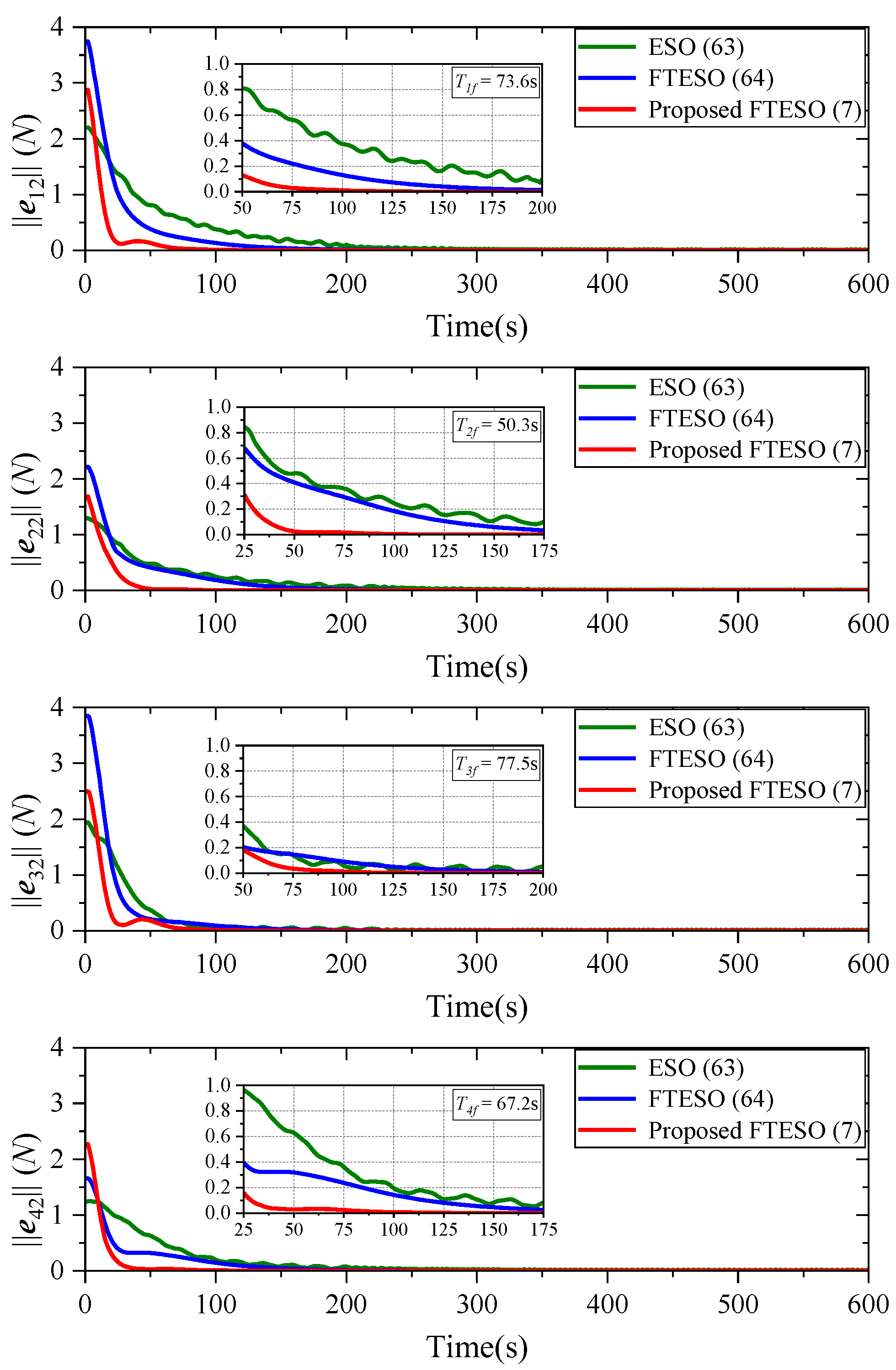
To verify the disturbance compensation performance of the proposed FTESO (7), we conducted comparative simulations with the ESO (67) from [43] and the FTESO (68) from [18]. Figure 4 shows the norms of the compound disturbance estimation errors $‖e_{i2}‖=‖{\widehat{\tau }}_{id}-{\tau }_{id}‖$ for the four AUVs under the three observers, characterizing insights into transient and steady-state responses. We calculated the settling time of the designed FTESO in the simulation and highlighted it on the plots. It is clear from Figure 4 that our proposed third-order fast FTESO can achieve finite-time stabilization, with the estimation errors converging to a small neighborhood of the origin. And the dynamic convergence speed and estimation accuracy of the proposed FTESO are better than ESO (67) and FTESO (68) with less chattering. This shows the advantages of our approach. Thus, each AUV can accurately compensate for model uncertainties and external disturbances of its corresponding subsystem in finite time.

$$\left\{\begin{array}{l}{\dot{\widehat{z}}}_{i1}={\widehat{z}}_{i2}-{\beta }_{i1}{a}_{i1}{e}_{i1}+G_i\left({\eta }_i,v_i\right)+{\tau }_i\hfill \\ {\dot{\widehat{z}}}_{i2}=-{\beta }_{i1}^2{a}_{i2}{e}_{i1}\hfill \end{array}\right..$$

(67)

$$\left\{\begin{array}{l}{\dot{\widehat{z}}}_{i1}={\widehat{z}}_{i2}-{\beta }_{i1}si{g}^{3/4}\left(e_{i1}\right)+G_i\left({\eta }_i,v_i\right)+{\tau }_i\hfill \\ {\dot{\widehat{z}}}_{i2}=-{\beta }_{i2}si{g}^{1/2}\left(e_{i1}\right)\hfill \end{array}\right..$$

(68)

The collision avoidance performance of the AUV formation was tested via a set of comparison experiments with and without collision avoidance constraints based on our proposed scheme. Since the initial positions of the four AUVs are randomly distributed, the risk of collision is increased. The formation trajectory without collision avoidance constraints is shown in Figure 5 (top). Here, the four AUVs track the reference trajectory while keeping the preset shape, but AUV3 and AUV4 collide at 10 s, followed by a collision between AUV1 and AUV2 at 20 s. Specifically, as presented in Figure 6 (top), the relative distance between AUV1 and AUV2 during the formation configuration stage exceeds the safe distance, resulting in a collision. The same situation occurs with AUV3 and AUV4. However, when collision avoidance constraints are considered, the formation trajectory (shown in Figure 5 (bottom)) indicates that the four AUVs can perform the formation tracking task while avoiding collision during the configuration stage. The collision avoidance performance is visualized in Figure 6 (bottom), where the distances among AUVs within the detection zone are always greater than the safe distance, indicating that inter-vehicle collision avoidance can be achieved. Therefore, the proposed control scheme can provide real-time collision avoidance capability for AUV formation maneuvers.

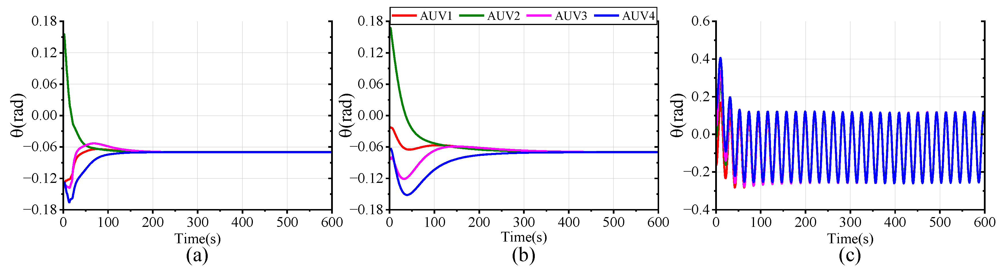
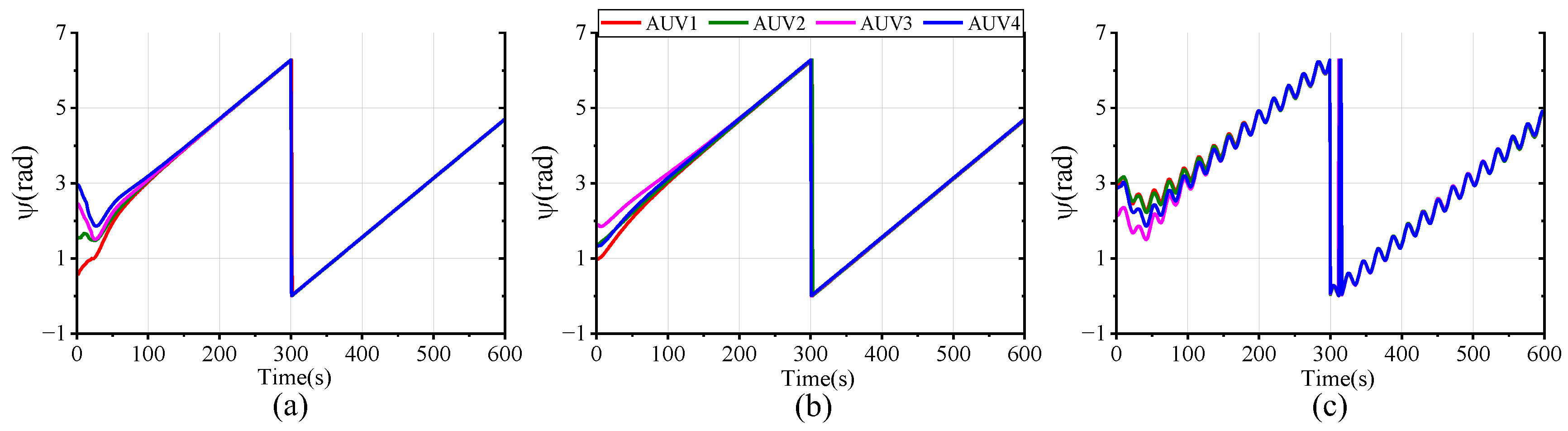
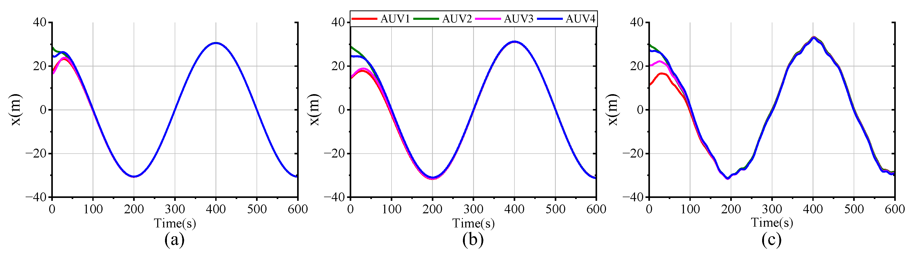
In order to assess the feasibility and superiority of the proposed scheme, we conducted three sets of comparative simulations with the same parameters, constraints, and disturbance settings: (a) the proposed FTESO-based dual closed-loop DMPC with Laguerre function; (b) a FTESO-based dual closed-loop DMPC without Laguerre function; (c) a standard DMPC without FTESO. 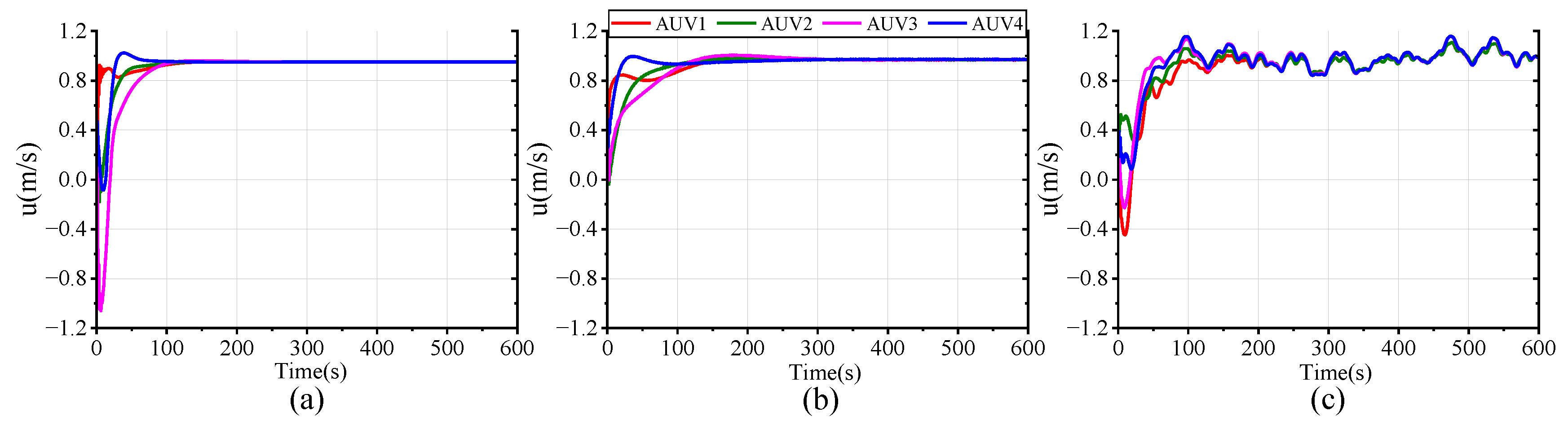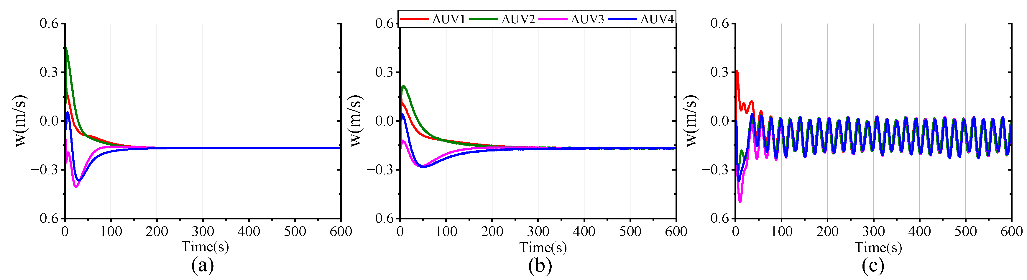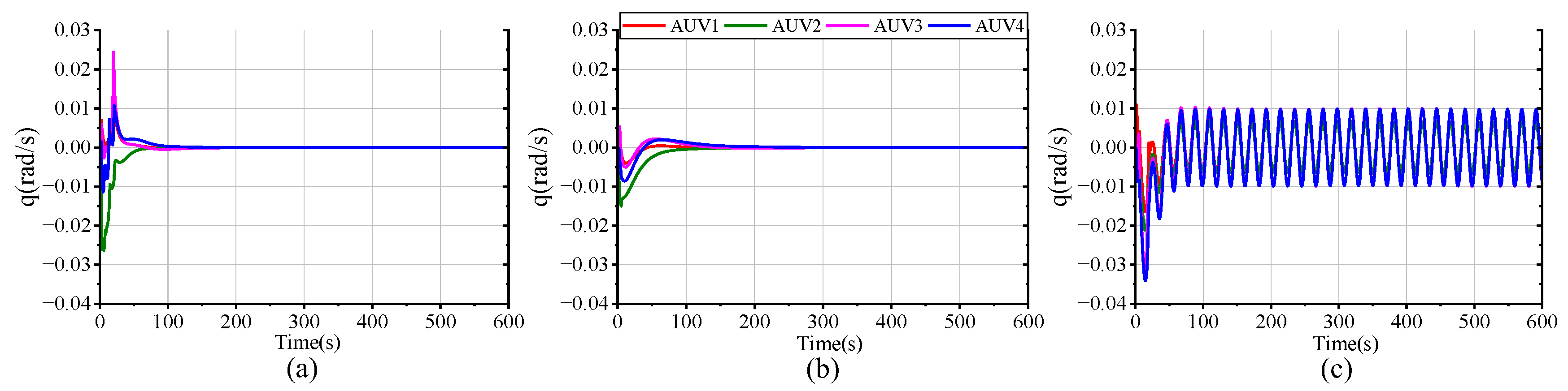Figure 7, Figure 8, Figure 9, Figure 10, Figure 11, Figure 12, Figure 13, Figure 14, Figure 15 and Figure 16 plot the tracking performance curves of AUV positional and velocity states under the three schemes. It can be easily observed that, in all scenarios, the four AUVs are able to successfully track the desired state despite the differing tracking errors. In scheme (a), full-state stable tracking is achieved within 200 s. Meanwhile, in scheme (b), the process takes about 300 s, which suggests that the use of the Laguerre function improves both the response speed and control accuracy. Although the standard DMPC scheme (c) can also achieve formation tracking, the settling time of the state variables is longer and accompanied by oscillations due to the uncompensated compound disturbance effects. Compared with the other schemes, our proposed method delivers superior formation tracking control performance.

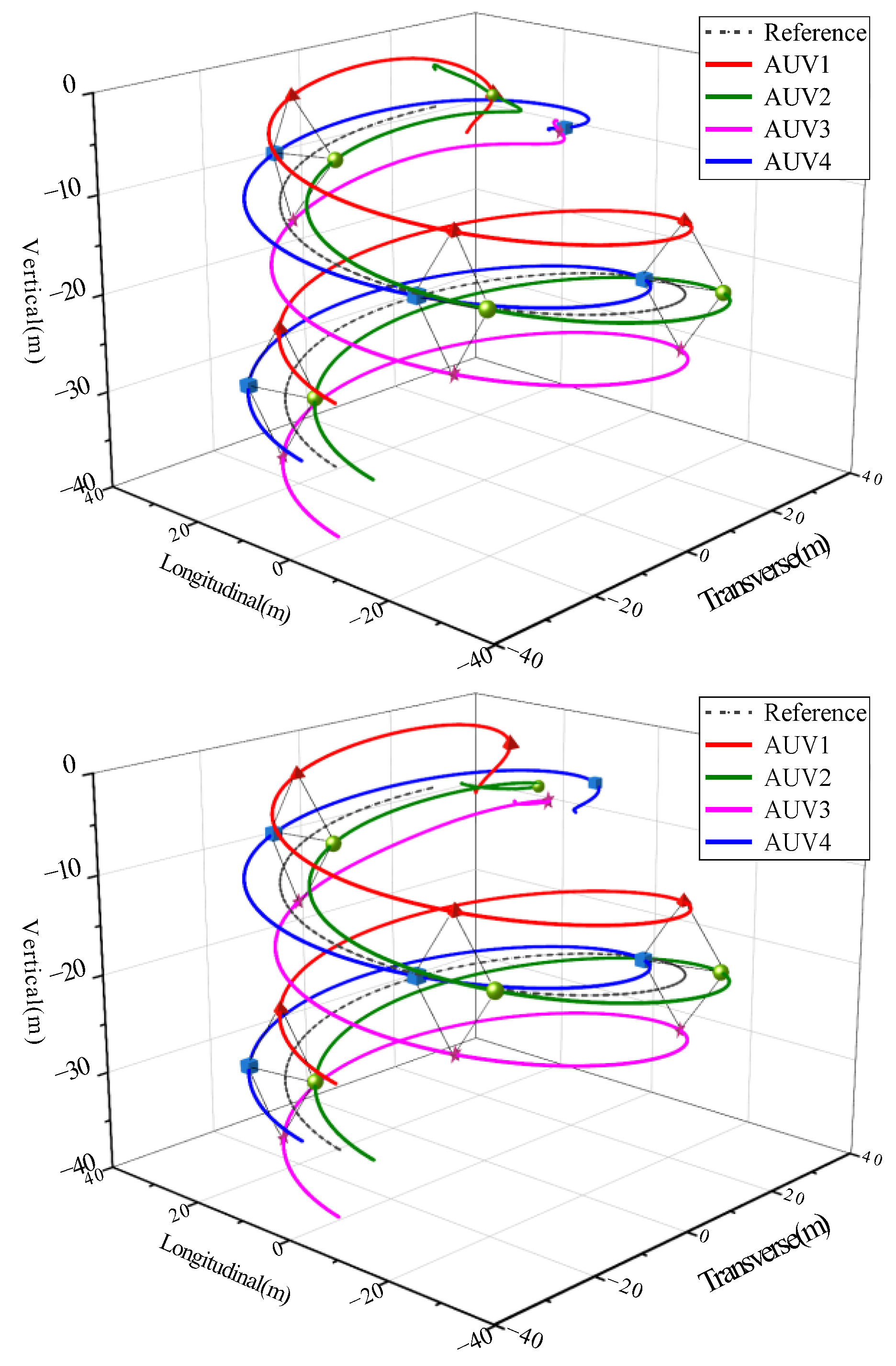
Figure 17 intuitively presents a 3-D formation trajectory tracking. Combined with Figure 7, Figure 8, Figure 9, Figure 10, Figure 11, Figure 12, Figure 13, Figure 14, Figure 15 and Figure 16, it implies that all three schemes can successfully accomplish formation spiral tracking under the specified input and state constraints. However, when the formation faces harsh compound disturbances, the tracking performance of the controller without disturbance compensation performs poorly, demonstrating a tracking error significantly larger than that of the FTESO-based controller. This is because the compound disturbances cause the AUV to deviate from the desired trajectory. By comparing the results of (a,b), it can be further observed that the proposed control scheme with Laguerre function allows the AUV to form the preset formation more quickly and converge to the desired trajectory more smoothly. This implies a faster response at the onset of the task. Thus, the dual closed-loop structure and Laguerre function enable the AUV formation to track the reference trajectory with better speed and accuracy.

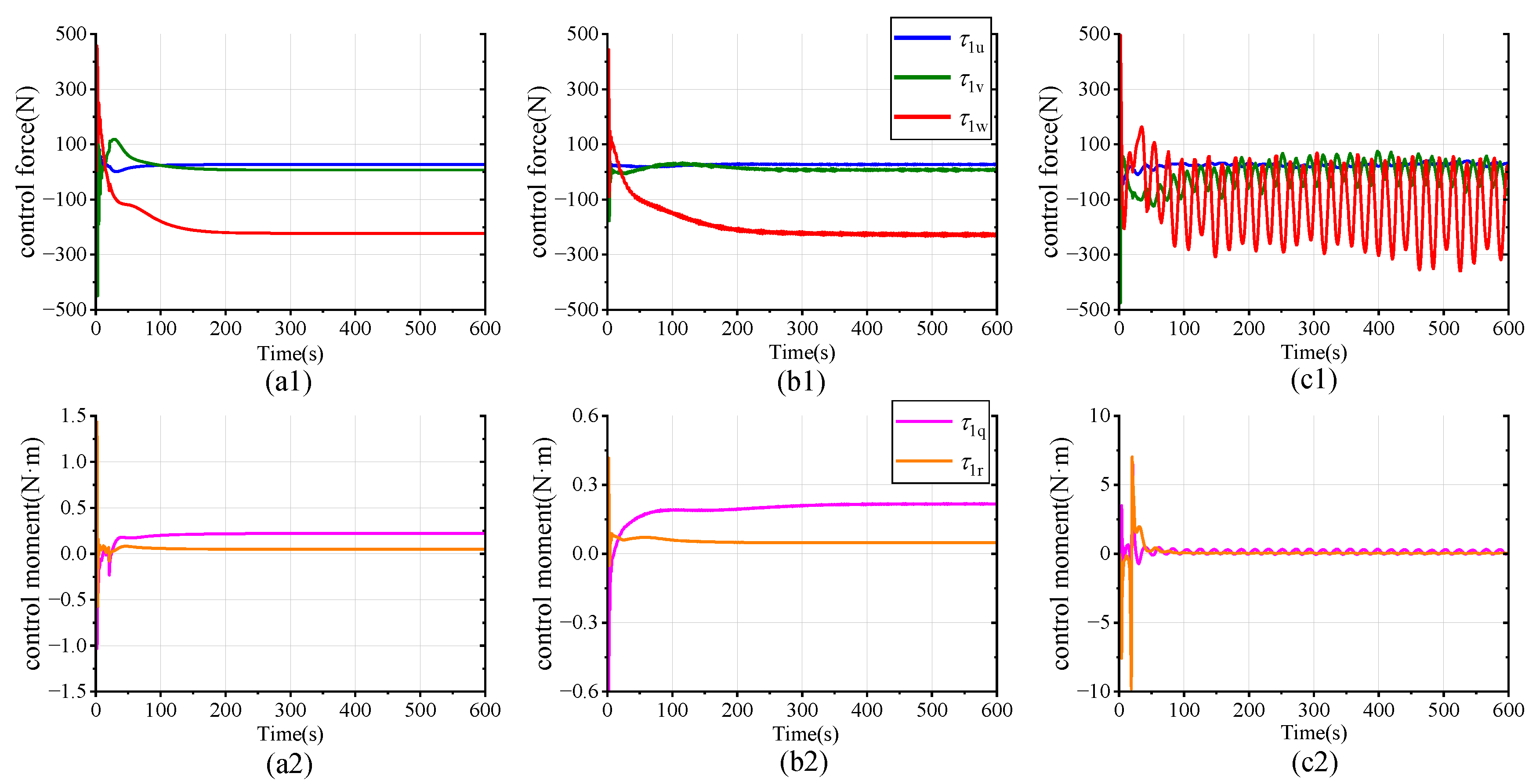
Without loss of generality, Figure 18 shows the actual control forces and moments versus time for AUV1 under the three schemes. Without the benefit of FTESO to compensate for compound disturbances, the fluctuations of the control force and moment are relatively drastic and unstable (Figure 18(c1,c2)). This is attributed to the need for the AUV to significantly rectify the driving forces and moments to more rapidly approach the deviated reference trajectory. Under the proposed scheme, as shown in Figure 18(a1,a2), the AUV forces and moments vary relatively smoothly, which makes the AUV track the trajectory steadily when disturbed. Comparing Figure 18(a1,a2) and Figure 18(b1,b2), the Laguerre-based controller has the fastest control signal response with the smallest amplitude when the disturbances are accurately compensated. This confirms that our proposed scheme (a) provides superior control performance. It is worth noting that the variation of control forces and moments always remains within the prescribed limits. This reflects the ability of the DMPC to handle the actuator saturation effectively, ensuring that the control input for each DOF does not exceed the maximum force provided by the actuator, thus reducing actuator losses.

To differentiate between the computational demands among the three schemes, we recorded the emulator execution times under the same configurations. The detailed simulation times corresponding to Figure 17 are given in

Table 2. Comparison of controller execution time.

Control Scheme	Simulation Time	Run Time
Scheme (a)	600 s	11.75 s
Scheme (b)	600 s	57.91 s
Scheme (c)	600 s	43.62 s

. It can be observed that the actual running time of the standard DMPC system is approximately 43.62 s. In contrast, the system with a dual closed-loop DMPC requires 57.91 s, which is about 32.8% longer than the standard DMPC. This increase is due to the greater complexity of the dual closed-loop structure as opposed to the simpler DMPC structure. Although there is improvement in control efficacy, the execution of the dual closed-loop structure is sacrificed to some extent. However, the proposed system, which employs a Laguerre-based dual closed-loop DMPC, the computation time only requires 11.75 s. This suggests that, despite the inclusion of both the dual closed-loop structure and FTESO, the use of the Laguerre function makes the system solution faster. Thus, the proposed scheme can simultaneously improve the computational speed and control performance.

5. Conclusions

In conclusion, this study presents a FTESO-based distributed dual closed-loop model predictive control scheme for the AUV formation subject to compound disturbances. The designed FTESO can compensate for model uncertainties and external disturbances of each AUV faster and more accurately. Control inputs are determined by solving a constrained DMPC optimization problem based on local information, while avoiding both collisions among AUVs and actuator saturation. The Laguerre orthogonal function is applied to alleviate the heavy computational burden, and the corresponding stability proof is provided. Finally, based on a connected directed topology, simulation results of different schemes are investigated under the same compound disturbances and system constraints. It is confirmed that our proposed scheme provides the best tracking effect and superior active disturbance rejection capability. Control signals show smaller oscillations and enhanced stability. In addition, the computation time of our proposed formation control system, which utilizes the Laguerre function, is reduced by 73.1% and 79.7% compared to the standard DMPC system and the dual closed-loop DMPC system, respectively. This verifies that our proposed scheme can respond quickly to minimize control costs and improve real-time execution and dynamic performance of the system.

The proposed method does not consider the impact of communication burden on AUV formation. Therefore, in future work, we will focus on the control scheme based on the event-triggered mechanisms. Considering the limitations of the optimization accuracy of discrete predictive control, we want to carry out research on continuous predictive control with faster control response. In addition, it is essential to conduct formation obstacle avoidance research and real AUV experiments.

References

1. Shi, Y.; Shen, C.; Fang, H.; Li, H. Advanced control in marine mechatronic systems: A survey. IEEE ASME Trans. Mechatron. 2017, 22, 1121–1131. [Google Scholar] [CrossRef]
2. Liu, G.; Chen, L.; Liu, K.; Luo, Y. A swarm of unmanned vehicles in the shallow ocean: A survey. Neurocomputing 2023, 531, 74–86. [Google Scholar] [CrossRef]
3. Yu, H.; Zeng, Z.; Guo, C. Coordinated formation control of discrete-time autonomous underwater vehicles under alterable communication topology with time-varying delay. J. Mar. Sci. Eng. 2022, 10, 712. [Google Scholar] [CrossRef]
4. Chen, Y.L.; Ma, X.W.; Bai, G.Q.; Sha, Y.; Liu, J. Multi-autonomous underwater vehicle formation control and cluster search using a fusion control strategy at complex underwater environment. Ocean Eng. 2020, 216, 108048. [Google Scholar] [CrossRef]
5. Zhen, Q.; Wan, L.; Li, Y.; Jiang, D. Formation control of a multi-AUVs system based on virtual structure and artificial potential field on SE(3). Ocean Eng. 2022, 253, 111148. [Google Scholar] [CrossRef]
6. Wang, J.; Wang, C.; Wei, Y.; Zhang, C. Sliding mode based neural adaptive formation control of underactuated AUVs with leader-follower strategy. Appl. Ocean Res. 2020, 94, 101971. [Google Scholar] [CrossRef]
7. He, X.; Geng, Z. Globally convergent leaderless formation control for unicycle-type mobile robots. IET Contr. Theory Appl. 2020, 14, 2651–2662. [Google Scholar] [CrossRef]
8. Munir, M.; Khan, Q.; Ullah, S.; Syeda, T.M.; Algethami, A.A. Control Design for Uncertain Higher-Order Networked Nonlinear Systems via an Arbitrary Order Finite-Time Sliding Mode Control Law. Sensors 2022, 22, 2748. [Google Scholar] [CrossRef]
9. Ullah, S.; Khan, Q.; Mehmood, A.; Kirmani, S.A.M.; Mechali, O. Neuro-adaptive fast integral terminal sliding mode control design with variable gain robust exact differentiator for under-actuated quadcopter UAV. ISA Trans. 2022, 120, 293–304. [Google Scholar] [CrossRef]
10. Zhang, W.; Wu, W.; Li, Z.; Du, X.; Yan, Z. Three-Dimensional Trajectory Tracking of AUV Based on Nonsingular Terminal Sliding Mode and Active Disturbance Rejection Decoupling Control. J. Mar. Sci. Eng. 2023, 11, 959. [Google Scholar] [CrossRef]
11. Cui, R.; Chen, L.; Yang, C.; Chen, M. Extended state observer-based integral sliding mode control for an underwater robot with unknown disturbances and uncertain nonlinearities. IEEE Trans. Ind. Electron. 2017, 64, 6785–6795. [Google Scholar] [CrossRef]
12. Ding, S.; Chen, W.H.; Mei, K.; Murray-Smith, D.J. Disturbance observer design for nonlinear systems represented by input-output models. IEEE Trans. Ind. Electron. 2019, 67, 1222–1232. [Google Scholar] [CrossRef]
13. Liang, X.; Qu, X.; Wan, L.; Ma, Q. Three-dimensional path following of an underactuated AUV based on fuzzy backstepping sliding mode control. Int. J. Fuzzy Syst. 2018, 20, 640–649. [Google Scholar] [CrossRef]
14. Zhang, G.; Yin, S.; Huang, C.; Zhang, W. Intervehicle Security-Based Robust Neural Formation Control for Multiple USVs via APS Guidance. J. Mar. Sci. Eng. 2023, 11, 1020. [Google Scholar] [CrossRef]
15. Han, J. From PID to active disturbance rejection control. IEEE Trans. Ind. Electron. 2009, 56, 900–906. [Google Scholar] [CrossRef]
16. Lei, M.; Li, Y.; Pang, S. Extended state observer-based composite-system control for trajectory tracking of underactuated AUVs. Appl. Ocean Res. 2021, 112, 102694. [Google Scholar] [CrossRef]
17. Nie, J.; Wang, H.; Lu, X.; Lin, X.; Sheng, C.; Zhang, Z.; Song, S. Finite-time output feedback path following control of underactuated MSV based on FTESO. Ocean Eng. 2021, 224, 108660. [Google Scholar] [CrossRef]
18. Wang, N.; Zhu, Z.; Qin, H.; Deng, Z.; Sun, Y. Finite-time extended state observer-based exact tracking control of an unmanned surface vehicle. Int. J. Robust Nonlinear Control. 2021, 31, 1704–1719. [Google Scholar] [CrossRef]
19. Sankaranarayanan, V.N.; Yadav, R.D.; Swayampakula, R.K.; Ganguly, S.; Roy, S. Robustifying payload carrying operations for quadrotors under time-varying state constraints and uncertainty. IEEE Robot. Autom. Lett. 2022, 7, 4885–4892. [Google Scholar] [CrossRef]
20. Chu, Z.; Xiang, X.; Zhu, D.; Luo, C.; Xie, D. Adaptive fuzzy sliding mode diving control for autonomous underwater vehicle with input constraint. Int. J. Fuzzy Syst. 2018, 20, 1460–1469. [Google Scholar] [CrossRef]
21. Li, S.; Wang, X. Finite-time consensus and collision avoidance control algorithms for multiple AUVs. Automatica 2013, 49, 3359–3367. [Google Scholar] [CrossRef]
22. Xu, J.; Huang, F.; Wu, D.; Cui, Y.; Yan, Z.; Du, X. A learning method for AUV collision avoidance through deep reinforcement learning. Ocean Eng. 2022, 260, 112038. [Google Scholar] [CrossRef]
23. Zhang, Y.; Liu, X.; Luo, M.; Yang, C. MPC-based 3-D trajectory tracking for an autonomous underwater vehicle with constraints in complex ocean environments. Ocean Eng. 2019, 189, 106309. [Google Scholar] [CrossRef]
24. Arcos-Legarda, J.; Gutiérrez, Á. Robust Model Predictive Control Based on Active Disturbance Rejection Control for a Robotic Autonomous Underwater Vehicle. J. Mar. Sci. Eng. 2023, 11, 929. [Google Scholar] [CrossRef]
25. Zheng, Y.; Li, S.E.; Li, K.; Borrelli, F.; Hedrick, J.K. Distributed model predictive control for heterogeneous vehicle platoons under unidirectional topologies. IEEE Trans. Control Syst. Technol. 2016, 25, 899–910. [Google Scholar] [CrossRef]
26. Wei, H.; Shen, C.; Shi, Y. Distributed Lyapunov-based model predictive formation tracking control for autonomous underwater vehicles subject to disturbances. IEEE Trans. Syst. Man Cybern. Syst. 2019, 51, 5198–5208. [Google Scholar] [CrossRef]
27. Shen, C.; Shi, Y. Distributed implementation of nonlinear model predictive control for AUV trajectory tracking. Automatica 2020, 115, 108863. [Google Scholar] [CrossRef]
28. Li, B.; Hu, Q.; Yu, Y.; Ma, G. Observer-based fault-tolerant attitude control for rigid spacecraft. IEEE Trans. Aerosp. Electron. Syst. 2017, 53, 2572–2582. [Google Scholar] [CrossRef]
29. Wei, H.; Sun, Q.; Chen, J.; Shi, Y. Robust distributed model predictive platooning control for heterogeneous autonomous surface vehicles. Control Eng. Pract. 2021, 107, 104655. [Google Scholar] [CrossRef]
30. Zhao, R.; Miao, M.; Lu, J.; Wang, Y.; Li, D. Formation control of multiple underwater robots based on ADMM distributed model predictive control. Ocean Eng. 2022, 257, 111585. [Google Scholar] [CrossRef]
31. Hu, Q.; Jiang, B. Continuous finite-time attitude control for rigid spacecraft based on angular velocity observer. IEEE Trans. Aerosp. Electron. Syst. 2018, 54, 1082–1092. [Google Scholar] [CrossRef]
32. Yan, Z.; Gong, P.; Zhang, W.; Li, Z.; Teng, Y. Autonomous underwater vehicle vision guided docking experiments based on L-shaped light array. IEEE Access 2019, 7, 72567–72576. [Google Scholar] [CrossRef]
33. Fossen, T.I. Handbook of Marine Craft Hydrodynamics and Motion Control; John Wiley & Sons: Hoboken, NJ, USA, 2011. [Google Scholar]
34. Xu, J.; Cui, Y.; Xing, W.; Huang, F.; Yan, Z.; Wu, D.; Chen, T. Anti-disturbance fault-tolerant formation containment control for multiple autonomous underwater vehicles with actuator faults. Ocean Eng. 2022, 266, 112924. [Google Scholar] [CrossRef]
35. Tao, T.; Roy, S.; De Schutter, B.; Baldi, S. Distributed Adaptive Synchronization in Euler Lagrange Networks with Uncertain Interconnections. IEEE Trans. Autom. Control, 2013; online ahead of print. [Google Scholar]
36. Roy, S.; Baldi, S.; Fridman, L.M. On adaptive sliding mode control without a priori bounded uncertainty. Automatica 2020, 111, 108650. [Google Scholar] [CrossRef]
37. Kong, S.; Sun, J.; Wang, J.; Zhou, Z.; Shao, J.; Yu, J. Piecewise Compensation Model Predictive Governor Combined with Conditional Disturbance Negation for Underactuated AUV Tracking Control. IEEE Trans. Ind. Electron. 2022, 70, 6191–6200. [Google Scholar] [CrossRef]
38. Wang, L. Continuous time model predictive control design using orthonormal functions. Int. J. Control. 2001, 74, 1588–1600. [Google Scholar] [CrossRef]
39. Yan, Z.; Wang, M.; Xu, J. Integrated guidance and control strategy for homing of unmanned underwater vehicles. J. Frankl. Inst.-Eng. Appl. Math. 2019, 356, 3831–3848. [Google Scholar] [CrossRef]
40. Hosen, M.A.; Hussain, M.A.; Mjalli, F.S. Control of polystyrene batch reactors using neural network based model predictive control (NNMPC): An experimental investigation. Control Eng. Pract. 2011, 19, 454–467. [Google Scholar] [CrossRef]
41. Cortes, P.; Kouro, S.; La Rocca, B.; Vargas, R.; Rodriguez, J.; Leon, J.I.; Vazquez, S.; Franquelo, L.G. Guidelines for weighting factors design in Model Predictive Control of power converters and drives. In Proceedings of the IEEE International Conference on Industrial Technology, Churchill, VIC, Australia, 10–13 February 2009; pp. 1–7. [Google Scholar]
42. Zhang, C.; Zhang, G.; Dong, Q. Multi-variable finite-time observer-based adaptive-gain sliding mode control for fixed-wing UAV. IET Contr. Theory Appl. 2021, 15, 223–247. [Google Scholar] [CrossRef]
43. Ma, C.; Tang, Y.; Lei, M.; Jiang, D.; Luo, W. Trajectory tracking control for autonomous underwater vehicle with disturbances and input saturation based on contraction theory. Ocean Eng. 2022, 266, 112731. [Google Scholar] [CrossRef]
Figure 1. AUV coordinate system.
Jmse 11 01897 g001
Figure 2. The FTESO-based DMPC dual closed-loop structure for the AUV formation.
Jmse 11 01897 g002
Figure 3. Structure of communication topology.
Jmse 11 01897 g003
Figure 4. Compound disturbance estimation errors e i 2 of the ith AUV.
Jmse 11 01897 g004
Figure 5. 3-D formation trajectories without (top) and with (bottom) collision avoidance constraints.
Jmse 11 01897 g005
Figure 6. Relative distances among AUVs without (top) and with (bottom) collision avoidance constraints.
Jmse 11 01897 g006
Figure 7. State x i of the AUV formation system. (a) The proposed FTESO-based dual closed-loop DMPC with Laguerre function. (b) The FTESO-based dual closed-loop DMPC without Laguerre function. (c) The standard DMPC without FTESO.
Jmse 11 01897 g007
Figure 8. State y i of the AUV formation system. (a) The proposed FTESO-based dual closed-loop DMPC with Laguerre function. (b) The FTESO-based dual closed-loop DMPC without Laguerre function. (c) The standard DMPC without FTESO.
Jmse 11 01897 g008
Figure 9. State z i of the AUV formation system. (a) The proposed FTESO-based dual closed-loop DMPC with Laguerre function. (b) The FTESO-based dual closed-loop DMPC without Laguerre function. (c) The standard DMPC without FTESO.
Jmse 11 01897 g009
Figure 10. State θ i of the AUV formation system. (a) The proposed FTESO-based dual closed-loop DMPC with Laguerre function. (b) The FTESO-based dual closed-loop DMPC without Laguerre function. (c) The standard DMPC without FTESO.
Jmse 11 01897 g010
Figure 11. State ψ i of the AUV formation system. (a) The proposed FTESO-based dual closed-loop DMPC with Laguerre function. (b) The FTESO-based dual closed-loop DMPC without Laguerre function. (c) The standard DMPC without FTESO.
Jmse 11 01897 g011
Figure 12. State u i of the AUV formation system. (a) The proposed FTESO-based dual closed-loop DMPC with Laguerre function. (b) The FTESO-based dual closed-loop DMPC without Laguerre function. (c) The standard DMPC without FTESO.
Jmse 11 01897 g012
Figure 13. State v i of the AUV formation system. (a) The proposed FTESO-based dual closed-loop DMPC with Laguerre function. (b) The FTESO-based dual closed-loop DMPC without Laguerre function. (c) The standard DMPC without FTESO.
Jmse 11 01897 g013
Figure 14. State w i of the AUV formation system. (a) The proposed FTESO-based dual closed-loop DMPC with Laguerre function. (b) The FTESO-based dual closed-loop DMPC without Laguerre function. (c) The standard DMPC without FTESO.
Jmse 11 01897 g014
Figure 15. State q i of the AUV formation system. (a) The proposed FTESO-based dual closed-loop DMPC with Laguerre function. (b) The FTESO-based dual closed-loop DMPC without Laguerre function. (c) The standard DMPC without FTESO.
Jmse 11 01897 g015
Figure 16. State r i of the AUV formation system. (a) The proposed FTESO-based dual closed-loop DMPC with Laguerre function. (b) The FTESO-based dual closed-loop DMPC without Laguerre function. (c) The standard DMPC without FTESO.
Jmse 11 01897 g016
Figure 17. 3-D trajectories of the AUV formation under different schemes. (a) The proposed FTESO-based dual closed-loop DMPC with Laguerre function. (b) The FTESO-based dual closed-loop DMPC without Laguerre function. (c) The standard DMPC without FTESO.
Jmse 11 01897 g017
Figure 18. Actual control force and moment for AUV1 under different schemes. (a1) Control force of scheme (a). (a2) Control moments of scheme (a). (b1) Control force of scheme (b). (b2) Control moments of scheme (b). (c1) Control force of scheme (c). (c2) Control moments of scheme (c).
Jmse 11 01897 g018