Power Prediction of a 15,000 TEU Containership: Deep-Learning Algorithm Compared to a Physical Model

Abstract

The authors proposed a direct comparison between white- and black-box models to predict the engine brake power of a 15,000 TEU (twenty-foot equivalent unit) containership. A Simplified Naval Architecture Method (SNAM), based on limited operational data, was highly enhanced by including specific operational parameters. An OAT (one-at-a-time) sensitivity analysis was performed to recognize the influences of the most relevant parameters in the white-box model. The black-box method relied on a DNN (deep neural network) composed of two fully connected layers with 4092 and 8192 units. The network consisted of a feed-forward network, and it was fed by more than 12,000 samples of data, encompassing twenty-three input features. The test data were validated against realistic operational data obtained during specific operational windows. Our results agreed favorably with the results obtained for the DNN, which relied on sufficiently observed data for the physical model.

1. Introduction

1.1. The Importance of Power Determination

Reducing fuel consumption has gained in importance and has become a trendy research direction in the shipping industry. Hence, precise power requirements in the design process of newbuilds as well as in the operational analyses of existing ships is of practical interest for all stakeholders, as ships are the largest contributor to fuel consumption in the transportation industry [1]. Furthermore, the transported volume increases continuously, with heavy diesel oil still being the preferred fuel. From 1990 to 2020, the transported cargo by ships more than doubled [1]. According to estimates of the fourth Greenhouse Gas (GHG) study, carried out by the International Maritime Organization (IMO) in 2020, the shipping industry, with 1056 million tons of emitted CO₂, was responsible for 2.89% of the total global anthropogenic CO₂ emissions in 2018. Moreover, this study reported that CO₂ emissions increased 9.3% in 2018 compared to 2012 [2].

Within the MEPC 80, the IMO has updated its decarbonization goals to reduce total emissions by at least 70%, striving for 80% until 2050, compared to 2008 [3].

To reach these goals, various measures have been taken. With the development of the Ship Energy Efficiency Management Plan (SEEMP Part III), ships of 5000 gross tonnages (GTs) and above will have to measure and document how they achieve their carbon intensity indicator (CII) targets, coming into force in 2023 [4]. Global crises and the associated energy shortages, as well as the rising operating costs of ships, need to be considered to reduce fuel consumption. Consequently, increasing the energy efficiency of ships in operation as well as during the design process is of interest. In this regard, it has become of paramount importance to obtain reliable and accurate predictions of the fuel consumption to determine a ship’s power requirements.

1.2. Methods to Determine a Ship’s Required Power

Various methods and techniques have evolved over the last 100 years to determine a ship’s required power.

Table 1. Overview of methods to determine a ship’s required power.

Method	Advantages	Disadvantages	Literature
Admiralty coefficient	Simple, first estimate during the design process.	Rough method, no (operational) parameters included.	Gupta et al., 2021 [5]
Standard Series Data Holtrop–Mennen Guldhammer–Harvald Taylor–Gertler, Series 60 Hollenbach	Power requirements for a given hull form.	Background and scope of application must be known.	Holtrop and Mennen, 1982 [6] Guldhammer and Harvald, 1974 [7]. Hollenbach, 1998 [8]
Computational fluid dynamics (CFD) Reynolds-averaged Navier–Stokes (RANS) solver	Accounts for viscous and free-surface flows, predicts calm-water resistance in a few hours.	Time-consuming, advanced method, requires experience and knowledge.	Molland et al., 2017 [9]
Machine-learning methods (e.g., artificial neural networks (ANNs) and deep feed-forward networks (DFNs))	Effective method to predict data patterns and solve complex problems if sufficient training data are available. Learn and train collected fuel consumption data repeatedly. Simulate relationship between fuel consumption and input data [5].	Internal parameters affect output data. Difficult to identify problematic areas [10].	Fan et al., 2022 [10] Lee et al., 2021 [11]

presents a brief overview of these methods.

Multiple studies have been conducted. Fan et al. [10], for instance, reviewed many available analytical models to estimate a ship’s fuel consumption. The so-called white, black, and grey boxes, which primarily depend on the nature of the algorithm employed (i.e., artificial intelligence or physical model), were used to categorize the existing ship fuel consumption models.

In general, it appears that traditional methods and data series are helpful for a rough power determination during the design process, albeit only if datasets from similar ships are available. Optimum predictions may be achieved by relying on a combination of different methods. To respond to changes accurately, the method to predict a ship’s power and its fuel consumption should be fast and flexible. Moreover, ship operators should be able to adjust certain key parameters and to control their interaction during a voyage. Lee et al. [11] state that deducing a ship’s power from resistance is not applicable to actual ships and, therefore, data-driven models based on ocean environmental and ship operational data should be established. With a DNN (deep neural network) approach, all these requirements can be combined to precisely determine a ship’s required power.

Therefore, a definite trend in the field of naval architecture is noticeable, especially due to the availability of sophisticated computer resources and their developments. For instance, the IACS Rec. 173 [12] already allows the application of numerical methods to determine the reference speed in the framework of the EEXI (Energy Efficiency eXisting ship Index). Instead of model tests, these methods are increasingly preferred to determine ship resistance. As introduced above, statistical methods, such as those of Holtrop and Mennen [6] or Hollenbach [8], have been widely used in the last decades. Nevertheless, machine-learning models now represent a practical alternative that needs to be investigated to understand all possible benefits when applied in the industry. For instance, Lang et al. [13] compared several supervised machine-learning algorithms to model a ship’s required power. Zhou at al. [14] demonstrated that their machine-learning approach, based on nine feature inputs and incorporating a reasonable generalization effect, is a sufficiently accurate tool to predict the required propulsive power. Lee et al. [11] proposed a deep feed-forward neural network (DFN), which they applied to predict a ship’s power using deep-learning methods because these networks are able to tackle complicated issues more successfully than regression analyses if enough training data are available.

The scope of this paper was to further develop the SNAM (Simplified Naval Architecture Method) of La Ferlita et al. [15] by including additional parameters. Therefore, our present investigation considered a more accurate physical model. This model differed from our previous model in that several parameters were either directly determined via specific algorithms or were obtained from observed (measured) data, such as the ship’s draft, the apparent wind speed, etc. Furthermore, we increased our understanding regarding the performance and capability of the DNN approach by considering differing available datasets with new features and by comparing the results with (measured) data from the physical model.

2. Materials and Methods

Operational data and associated multiple parameters were collected and monitored over a period of one operational year for a representative containership. A two-stroke nine-cylinder diesel engine, model MAN 9G95, provided the ship’s main propulsive power.

Table 2. Principal particulars and engine characteristics of the subject containership.

Ship Particulars and Engine Characteristics	Value
LOA (m)	367.0
LPP (m)	350.0
Breadth (m)	51.0
Depth (m)	30.4
Design draft (m)	14.5
Displacement at design draft (tons)	194,878
Scantling draft (m)	15.5
M/E cylinders	9
DMCR (kW)	46,900
Propeller diameter (m)	10.0
Propeller pitch (m)	9.3

lists the ship principal particulars and engine characteristics.

The following twenty-three engine-related parameters were monitored to obtain continued measurements at fifteen-minute intervals of the machinery-related conditions:

• Boiler consumed (MT);
• DG consumed (MT);
• ME consumed (MT);
• DG electric power (kW);
• Shaft power (kW);
• Shaft rpm (rpm);
• Draft foreword (m);
• Draft aft (m);
• Relative/apparent wind speed (m/s);
• Relative wind direction (deg);
• COG heading (deg);
• GPS speed (knots);
• Log speed (knots);
• Shaft generator power (kW);
• Under-keel clearance (m);
• Shaft generator power (kW);
• DG1 power (kW);
• DG2 power (kW);
• DG3 power (kW);
• DG4 power (kW);
• Shaft torque (kNm);
• WHR—turbo-generated electric power (kW);
• ME power (KW).

2.1. The White-Box Model

2.1.1. Resistance in Calm Water and in Waves

Calm-water resistance was calculated according to the well-established method of Holtrop and Mennen [6]. Through the regression analysis of a wide range of model tests and trial data, the resistance is decomposed into several components, such as the following:

-

Frictional resistance;

-

Appendage resistance;

-

Wave resistance;

-

Resistance due to bulbous bow near the water surface;

-

Pressure resistance due to immersed transom;

-

Model–ship correlation resistance;

-

Air resistance.

Typically, predictions with such a method are reliable, as demonstrated by Elkafas et al. [16], who performed a computational fluid dynamics (CFD) simulation that compared favorably to the results of the Holtrop method [16]. Deshpande et al. [17] demonstrated that the results from the Holtrop–Mennen method agreed well with a CFD simulation, especially at low ship speeds [17]. To determine the added resistance in waves, we already embedded the STA-WAVE-1 formulation into our previous algorithm of La Ferlita et al. [15]. This approach is reliable under head-sea conditions, in which pitch and heave motions are minimal. Therefore, this formulation should only be utilized under generally favorable weather conditions.

However, other methods exist. Here, we considered the improved formulation of Papanikolaou [18]. This method decomposes the total added wave resistance into two components: the resistance ($R_{AWR}$) in regular waves due to diffraction, defined as follows:

$$R_{AWR}=2.25·\rho ·g·B·{\zeta }_a{}^2·si{n}^{2}E\left(1+5\sqrt{\frac{L_{pp}}{\lambda }}{F}_n\right){\left(\frac{0.87}{C_b}\right)}^{1+4\sqrt{F_n}}$$

(1)

and the added resistance ($R_{AWM}$) in regular waves due to the ship’s motion, defined as follows:

$$R_{AWM}=4·\rho ·g·{\zeta }_a{}^2·\frac{B^2}{L_{pp}}·{\omega }^{b1}·exp\left[\frac{b_1}{d_1}\left(1-{\overline{\omega }}^{d1}\right)\right]a_1{a}_2$$

(2)

where

• B is the breadth of the ship;
• ρ is the water density;
• ${\zeta }_a$ is the wave amplitude;
• $L_{pp}$ is the ship’s length between perpendiculars;
• $F_n$ is the Froude number;
• $\lambda$ is the wave length;
• $C_b$ is the block coefficient;
• $\omega$ is the circular wave frequency;
• $\overline{\omega }$ is the resonance frequency dependent on the Froude number;
• $b_1$ and $d_1$ are the factors defined in [18];
• $a_1$ is the peak-added-resistance factor;
• $a_2$ is the forward-speed factor.

The formulation of Papanikolaou is advantageous, as it is a simplified engineering formula suitable to satisfactorily estimate a ship’s added resistance in waves [18]. However, implementing this formulation is not a straightforward task because the nonlinear effects are not considered. However, CFD simulations that solve the Reynolds-averaged Navier–Stokes (RANS) equations are able to consider nonlinear effects and, therefore, provide more accurate overall predictions [19].

Wave scatter diagrams specify the ship’s operational sea areas. These diagrams present the joint distribution of sea states characterized by their significant wave heights and zero-uncrossing periods.

2.1.2. Added Resistance Due to Winds

It is well known that a ship encounters air and wind resistance while at sea, and this may have negative impacts when maneuvering in harbors or restricted areas. However, the greatest interest in terms of fuel usage is the resistance that the ship encounters when underway. Compared to other kinds of ships, a containership’s windage area depends strongly on its loading situation, due to the presence of deck containers and the ship’s superstructure.

Studies to understand such effects were performed by Blenderman et al. [20]. He systematically measured wind forces acting on scaled ship models placed in a wind tunnel. Based on regression and correlation analyses, he established functional relationships of the aerodynamic-load coefficients for ships with various superstructures at different incidence wind angles. Andersen [21] tested a 9000 TEU containership model with several container deck-load combinations at wind directions ranging between head and stern headings.

Although the air resistance component included in the Holtrop and Mennen method was available, the wind resistance (R_wind) was estimated more accurately using the formulation of Blendermann [22]:

$$R_{wind}=\frac{{\rho }_{air}}{2}·u^2·A_L·C{D}_l\frac{cos\epsilon }{1-\frac{\delta }{2}\left(1-\frac{C{D}_l}{C{D}_t}\right)si{n}^{2}2\epsilon }$$

(3)

where

• $\rho$ is the air density;
• $u$ is the apparent wind velocity;
• $A_L$ is the ship’s projected lateral area;
• $\delta$ is the cross-force parameter;
• $C{D}_l$ is the non-dimensional longitudinal drag coefficient;
• $C{D}_t$ is the non-dimensional transverse drag coefficient;
• $\epsilon$ is the apparent wind angle.

2.1.3. Efficiency Factors

Contrary to the assumptions applied above in the simplified method [15], here, the efficiency factors were directly calculated. For the transmission-shaft efficiency, a factor of 0.98 was considered as the machinery was positioned aft [23]. The following formulations were considered:

• The relative rotational efficiency (${\mathsf{\eta }}_{\mathrm{R}}$) was determined according to the formulation of Holtrop and Mennen for a single-screw ship:

$${\mathsf{\eta }}_{\mathrm{R}}=0.9922-0.05908·\frac{A_E}{A_O}+0.07424·\left(Cp-0.0225·l_{CB}\right)$$

(4)

where $\frac{A_E}{A_O}$ is the blade area ratio, $Cp$ is the prismatic coefficient, and $l_{CB}$ is the longitudinal position of the ship’s center of buoyancy;

• The open-water propeller efficiency (${\mathsf{\eta }}_{\mathrm{O}}$) was calculated as follows:

$${\mathsf{\eta }}_{\mathrm{O}}=\frac{K_T{J}_A}{K_{Q}2\pi }$$

(5)

where the advance ratio ($J_A$), obtained via the advance speed ($V_A$), the propeller diameter (D), the thrust coefficient ($K_T$), and the torque coefficient ($K_Q$) were determined via the following polynomial regression formulas:

$$J_A=\frac{V_A}{nD}$$

(6)

$$K_T={\displaystyle \sum }_{s,t,u, v}{C}_{s,t,u,v}^T{J}^S{\left(\frac{P}{D}\right)}^t{\left(\frac{A_E}{A_O}\right)}^u{z}^v$$

(7)

$$K_Q={\displaystyle \sum }_{s,t,u, v}{C}_{s,t,u,v}^Q{J}^S{\left(\frac{P}{D}\right)}^t{\left(\frac{A_E}{A_O}\right)}^u{z}^v$$

(8)

where $\frac{P}{D}$ is the pitch diameter ratio, z is the number of propeller blades, $C_{s,t,u,v}^T$ and $C_{s,t,u,v}^Q$ are the coefficients obtained via the polynomial regression formulas, and s, t, u, and v are the exponents given by Bernitsas et al. [24];

• The hull efficiency (${\mathsf{\eta }}_{\mathrm{H}}$) was determined as follows:

$${\mathsf{\eta }}_{\mathrm{H}}=\frac{1-t}{1-w}$$

(9)

where t is the thrust deduction factor, and $w$ is the wake fraction. Finally, the ship’s brake power ($P_B$) was obtained as follows:

$$P_B=\frac{R_{tot}·v_s}{{\mathsf{\eta }}_{tot}}$$

(10)

where $v_s$ is the ship speed, $R_{tot}$ is the total resistance, and ${\eta }_{tot}$ is the total efficiency factor.

2.2. The Black-Box-Model DNN

Deep neural networks (DNNs) are widely considered the most popular and powerful machine-learning method. They have been successfully applied in a variety of fields, such as computer vision, natural language processing, and speech recognition. DNNs are artificial neural networks (ANNs) that have multiple hidden layers. In DNNs, the number of hidden layers can reach 100 or more [25].

Often, the distribution and statistical properties of the input features are investigated to perform a data transformation beforehand, as indicated by Jiao et al. [26] and Ji et al. [27]. However, the DNN approach is itself an optimization process. As the weight of single features are independently updated until the algorithm finds the correct pattern and due to the necessity of a relevant number of samples and features, we did not consider this to be relevant and, therefore, neglected this statistical aspect in our analysis.

To develop the neural networks, Google Colab [28] and TensorFlow were used. Google Colab is a product from Google that allows the execution of an arbitrary Python code well suited to machine learning. TensorFlow is a deep-learning computational tool kit. DNNs employ input features, and they comprehend their initial and output values. These models contain learning and training processes.

The associated output is then described by a linear combination of an adjustable input and a bias [29]. After the computation, it is activated by a nonlinear function [25]. The DNN terminology represents the presence of multiple inner layers considered inside the network. The modeling method for a DNN is based on the back-propagating learning algorithm used in the backward step with two hidden layers [30]. In our proposed neural network, one layer consisted of 8192 activation units and the other layer consisted of 4096 activation units. The network structure was similar to the one already proposed by La Ferlita et al. [15], except for the input features. The same number of units for the first and second layers was considered, as in our previous study [15], because the amount of data available was similar and because the so-called curse of non-dimensionality [30] was taken into account. A network with many layers and a limited amount of data is more likely to deliver poor predictions.

The activation function was a swish nonlinear function [31], derived from the Sigmoid-weighted linear unit function, a continuous smooth function that permits a few negligible weights to be propagated in the network.

The optimizer algorithm ADAM was embedded. This algorithm is a further extension of a stochastic gradient descent used to update network weights during training. An optimizer represents a function or an algorithm that adjusts attributes of the neural network, such as weights and learning rates. Hence, for parameter updates (${\theta }_{t+1}$), the following equations (which rely on the concepts of gradient and momentum) are used in the package ADAM Algorithm [25]:

$$m_t={ß}_1{m}_{t-1}+\left(1-{ß}_1\right)g_t$$

(11)

$$v_t={ß}_2{v}_{t-1}+\left(1-{ß}_2\right)g_t^2$$

(12)

$$m_t^{^}=\left(\frac{m_t}{1-{ß}_1^t}\right)v_t^{^}=\left(\frac{v_t}{1-{ß}_2^t}\right)$$

(13)

$${\theta }_{t+1 }={\theta }_t-\frac{\eta }{\sqrt{v_t^{^}+ϵ}}{m}_t^{^}$$

(14)

where

• ${ß}_1$ and ${ß}_2$ are the exponential decay rates;
• $m_t$ is the exponential moving average of the gradient;
• $v_t$ is the exponential moving average of the squared gradient;
• $\theta$ is the network parameter to be updated;
• $g_t$ is the gradient;
• $m_t^{^}$ is the correction bias for $m_t$;
• $v_t^{^}$ is the correction bias for $v_t$;
• $\eta$ is the learning rate;
• $ϵ$ is a smoothing term that avoids division by zero.

Through this algorithm, the learning rate for each parameter is adjusted dynamically. The default values for ${ß}_1$ and ${ß}_2$ are 0.9 and 0.999, respectively. As performance metrics to understand the DNN capabilities, the two main parameters RMSE and MAE were considered [15]. The training and the validation steps were performed by splitting the training dataset, consisting of about 12,000 samples, with the usual 80/20 approach. Afterwards, the neural network was put to the test in brand new situations that were unknown to the algorithm.

3. Results and Discussion

We considered the two voyage scenarios A and B to test the physical model and the deep-learning approach. Scenario A represented a sea passage of about 72 h, and scenario B represented a sea passage of about 48 h. The first scenario referred to a voyage starting on the 7th of July and ending on the 10th of July through the Suez Canal (Figure 1). The second voyage referred to a voyage starting on the 10th of September and ending on the 12th of September within the South China Sea area (Figure 2).

Figure 3 and Figure 4 present the time histories of the calculated brake powers obtained for the two sea-passage scenarios, A and B, respectively. The vertical axis marks the brake power expressed in kW, while the horizontal axis represents the chronological sample points recorded every 15 min. Black lines mark the observed brake power, red lines mark the brake power determined via the physical method, and blue lines mark the brake power predicted via the DNN approach.

For scenario A, the brake power obtained from the DNN behaved qualitatively like the observed (measured) brake power. The predicted brake power from the physical model, however, fluctuated somewhat, especially over the first 120 sample points. At sample point 75, the physical model predicted a downward peak.

Between sample points 80 and 120, the brake power from the DNN approach deviated from the observed brake power. Generally, the physical model underpredicted the observed brake power.

For scenario B, both the physical model as well as the DNN approach delivered accurate brake power predictions over the first 20 sample points. At sample point 25, the physical model clearly underestimated the observed (measured) brake power. Starting from sample point 50 until sample point 80, the physical model overestimated the observed (measured) brake power as well as the brake power predicted by the DNN approach. Starting from sample point 80, the physical model as well as the DNN approach underestimated the observed (measured) brake power. However, starting from sample point 250, the DNN approach delivered brake power predictions that compared more favorably to the observed (measured) brake power predictions.

In general, the brake power obtained from the physical model and the DNN approach slightly underpredicted the observed (measured) brake power; however, the lesser brake power fluctuations from the DNN approach agreed more favorably with the observed (measured) brake power. The partial dataset can be found in the Supplementary Materials related to this article.

The features available in the DNN approach, together with the associated input data that were not filtered before proceeding with training the model, delivered accurate predictions. The somewhat less accurate predictions were attributable to the lack of training data samples necessary to identify the observed (measured) values.

In general, the physical model tended to simulate a dynamic system with external conditions varying every 15 min. For instance, the relevant values related to the added resistance in waves, such as the peak period and wave amplitude, were not available in the measured dataset. Therefore, these inputs were not adjusted, but they did affect the predictions. For the DNN approach, this was not the case because the model was not adjusted manually, and because the effects of the external conditions tuned the values independently. In addition, this physical model might not be accurate for all types of vessels; hence, some deviations for a particular ship’s topology could occur.

Furthermore, to qualitatively understand and visualize the results from a statistical perspective, Figure 5 presents scatter graphs, plotting the actual ship power versus the predicted power obtained with both methods. These scatter graphs visualize the model’s predictive accuracy together with the associated outliers. For scenario A, the two approaches obtained many data points that fit the regression equation, yielding R-squared values of 0.09825 and 0.9655, respectively, as shown in Figure 5a,b. For scenario B, many points deviated from the regression equation, especially at lower values of power, yielding R-squared values of 0.8676 and 0.7371, respectively, as shown in Figure 5c,d. This was attributable to the flaws of the two models, as they both underestimated the observed (measured) values.

Table 3. Normalized RMSEs and MAEs for the physical model and the DNN method.

Scenario	Normalized RMSE (Physical Model)	Normalized RMSE (DNN Method)	Normalized MAE (Physical Model)	Normalized MAE (DNN Method)
A	0.0465	0.0177	0.0422	0.0151
B	0.0344	0.0242	0.0300	0.0202

summarizes the results for the two scenarios in terms of the normalized Root-Mean-Squared Errors (RMSEs) and normalized MAEs (Mean Average Errors).

Compared to the DNN approach, the physical model predicted brake power values that agreed less closely with the reported values. For the first scenario, the DNN approach yielded an RMSE value of 0.0465 and an MAE value of 0.0422. As seen in Table 3, for the second scenario, the relatively low MAE and RMSE values obtained for the DNN method turned out to be 0.0202 and 0.0242, respectively. Despite the relatively low amount of data used to train the algorithms, the network’s predictions agreed favorably compared to the physical model.

4. Sensitivity Analysis

Employing the OAT (one-at-a-time) method, we performed a sensitivity analysis to qualitatively assess the brake power predictions. One variable was modified by varying it a certain amount while maintaining the other variables constant. The modified variable was then reset to its nominal value after the simulation. This strategy did not consider possible interactions between variables.

The advantage of using the OAT method was that any observable changes in the model could be attributed to a change of just one factor. This method was simple compared to other multi-factor sensitivity analysis methods and, in addition, it was computationally efficient.

The modified parameters were chosen to simplify the large number of variables present in the physical algorithm. Furthermore, these parameters were categorized into the following macrogroups: calm-water resistance, added resistance in waves, added resistance due to winds, and efficiency factors. Figure 6 presents the associated box plots within the framework of the sensitivity analysis for a test scenario consisting of 73 samples representing one day of a sea passage. The ordinate of the box plots refers to the ship’s brake power; the abscissa refers to the non-dimensional default values of the wave amplitude, propeller diameter, ship draft, ship breadth, ship-hull lateral drag coefficient, ship speed, shaft efficiency, peak period of the seaway, ship length between perpendiculars, and ship projected lateral area.

The ship geometric parameters applied in the physical model, such as the ship length between perpendiculars (Figure 6i) and ship breadth (Figure 6d), hardly influenced the outcome in terms of the brake power. However, the ship’s projected lateral drag coefficient (Figure 6e) and, to a lesser extent, its lateral projected area (Figure 6j), did affect the brake power because these parameters determined the wind-load resistance. By varying the lateral drag coefficient, the brake power reached values of up to 38,000 kW, whereas varying the lateral area did not significantly contribute to increasing the brake power. Indeed, it remained constant at about 28,000 kW. The influence of varying the ship’s speed on the brake power (Figure 6f) was as expected, generally following the cubic relationship between power and speed. The default values related to the added resistance in waves, (i.e., the seaway’s wave amplitude (Figure 6a) and peak period (Figure 6h)) played an important role in the model. The wave amplitude varied almost linearly with the brake power, and the seaway’s peak period varied almost sinusoidally with the brake power. The effect of the propeller diameter (Figure 6b) was similar to the effect of the wave amplitude.

The shaft efficiency, having been set to 0.98, affected the overall model performance, as it led to an unrealistically high-power demand with the risk of causing a defect in the mechanical propulsion system. A greater draft (Figure 6c) increased the brake power, thereby highlighting the sensitivity of the analysis in assessing the brake power predictions. A greater draft increased the wetted surface area markedly. Specifically, doubling the ship’s draft compared to its nominal draft led to a brake power requirement of 41,000 kW.

5. Conclusions

The simplified SNAM (Simplified Naval Architecture Method), established on sound principles of naval architecture, was further enhanced by embedding new input parameters and improving the physical algorithm to predict the operational brake power of a 15,000 TEU containership. In parallel, a DNN (deep neural network) was developed and is presented. The conclusions are summarized as follows:

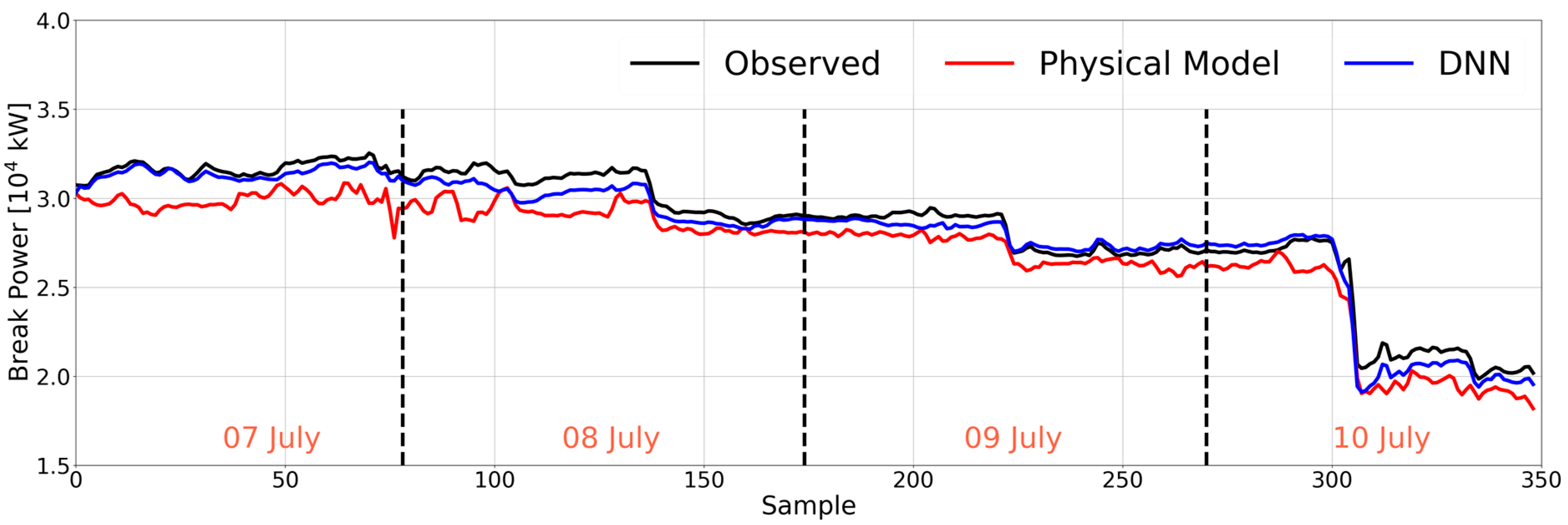
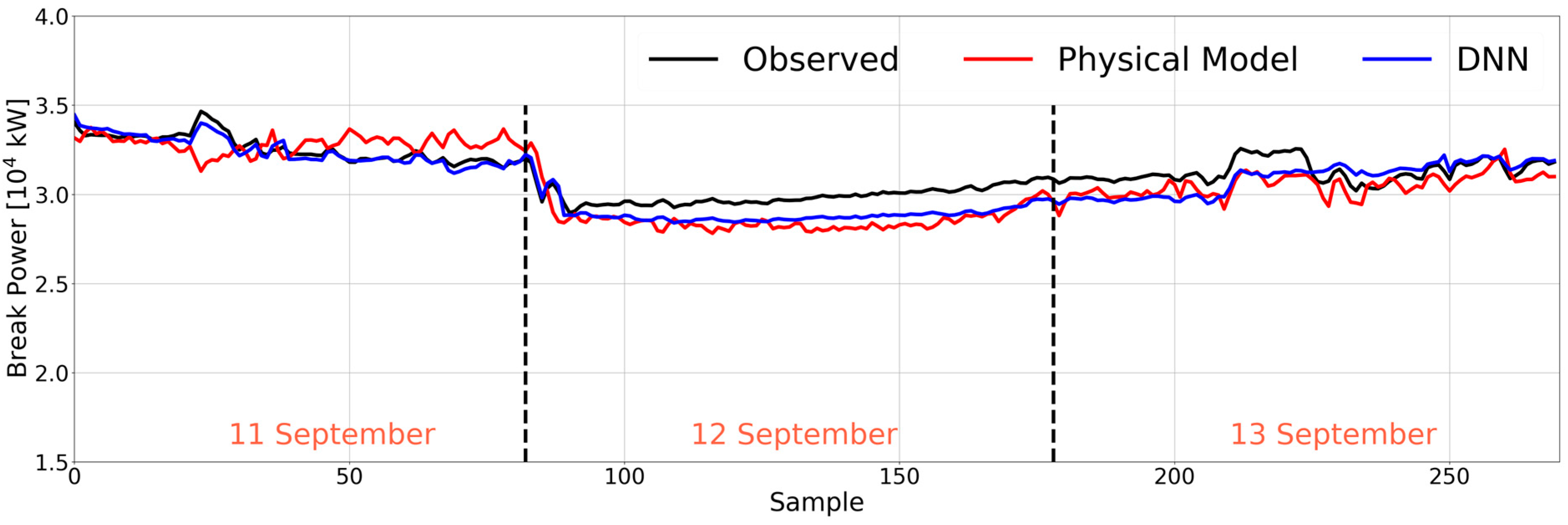
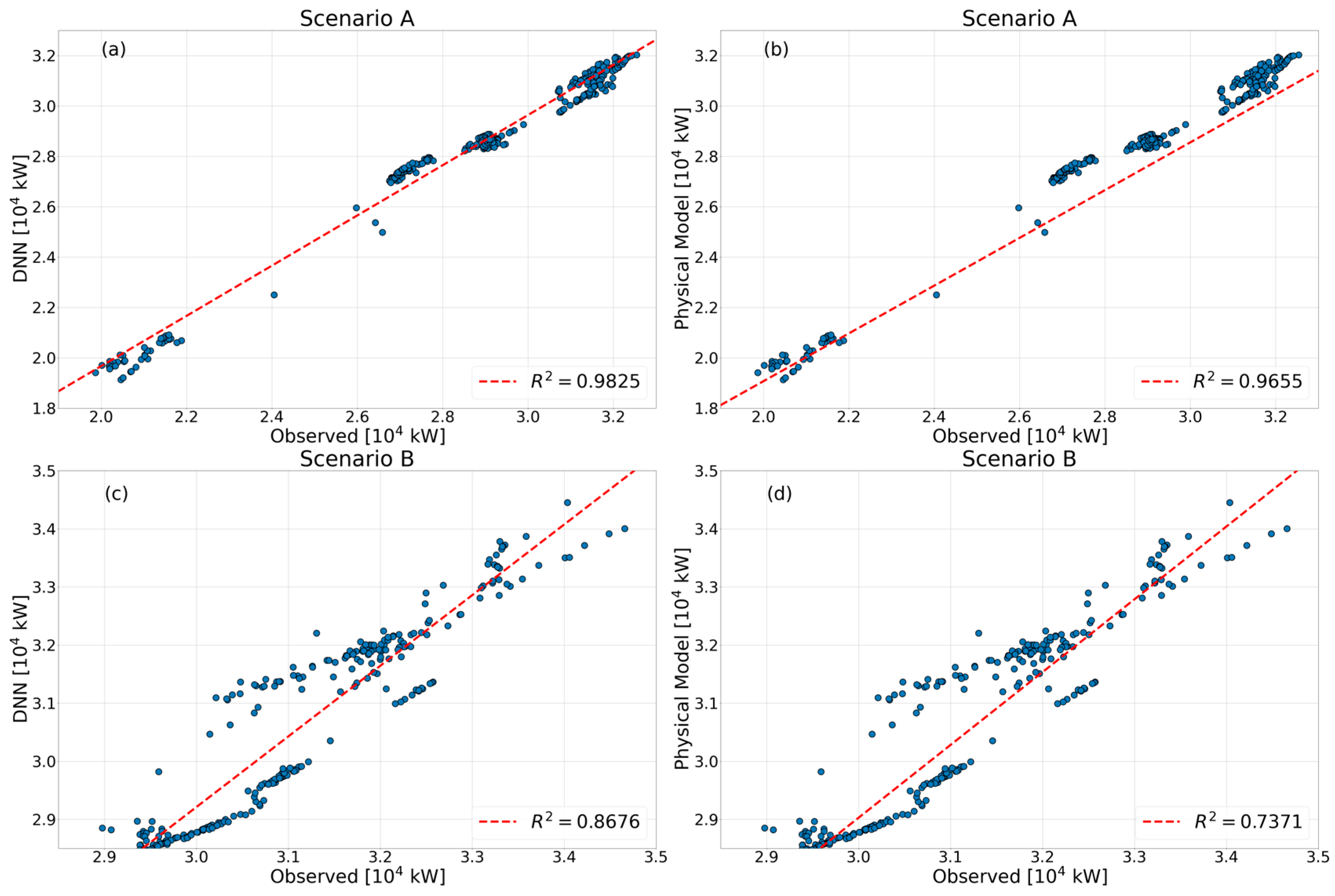
• Generally, our brake power predictions from the DNN compared more favorably to the observed (measured) predictions than those obtained from the enhanced SNAM. The RMSE, the MAE, as well as the R-square approaches obtained more accurate predictions than the physical model;
• More frequent fluctuations characterized the enhanced SNAM predictions, despite the more accurate formulations of, for example, the added resistance in waves and wind resistance. The RMSE and MAE approaches yielded lower values for the two scenarios presented. By and large, several parameters were defined in advance for the physical method proposed in our white-box model. This meant that the values inside the physical approach could not be adjusted during the scenarios, which led to underpredictions in some cases;
• Our results demonstrated the practical feasibility of this machine-learning DNN approach, considering the increased number of input features compared to the previous data-driven approach of ours, lowering the RMSE values as well.

In the future, we plan to investigate the application of more sophisticated approaches, such as CFD methods, to obtain highly accurate predictions, which will then be compared with predictions from the machine-learning model. Specifically, we plan to extract the independent variables in advance and to correlate these via an appropriate statistical analysis.

References

1. Placek, M.; «Ocean Shipping Worldwide—Statistics & Facts» Statista. 20 June 2022. Available online: https://www.statista.com/topics/1728/ocean-shipping/#topicOverview (accessed on 25 May 2023).
2. IMO. 4th Greenhouse Gas (GHG) Report. 2020. Available online: https://www.imo.org/en/ourwork/Environment/Pages/Fourth-IMO-Greenhouse-Gas-Study-2020.aspx (accessed on 20 July 2023).
3. IMO. Marine Environment Protection Committee (MEPC 80), 3–7 July 2023. Available online: https://www.imo.org/en/MediaCentre/MeetingSummaries/Pages/MEPC-80.aspx#:~:text=7%20July%202023-,Marine%20Environ-ment%20Protection%20Committee%20(MEPC,)%2C%203%2D7%20July%202023&text=The%20MEPC%2080%20session%20adopted,targets%20to%20tackle%20harmful%20emissions (accessed on 23 July 2023).
4. IMO. RESOLUTION MEPC.353(78). 2022. Available online: https://wwwcdn.imo.org/localresources/en/OurWork/Environment/Documents/Air%20pollution/MEPC.353(78).pdf (accessed on 28 March 2023).
5. Gupta, P.; Taskar, B.; Steen, S.; Rasheed, A. Statistical modeling of Ship’s hydrodynamic performance indicator. Appl. Ocean. Res. 2021, 111, 102623. [Google Scholar] [CrossRef]
6. Holtrop, J.; Mennen, G. An approximate power prediction method. Int. Shipbuild. Prog. 1982, 29, 166–170. [Google Scholar] [CrossRef]
7. Guldhammer, H.E.; Harvald, S.A. Ship Resistance—Effect of Form and Principal Dimensions; Danish Technial Press: Copenhagen, Denmark, 1974. [Google Scholar]
8. Hollenbach, K. Estimating resistance and propulsion for single-screw and twin-screw ships. Ship Technol. Res. 1998, 45, 72–76. [Google Scholar]
9. Molland, A.; Turnock, S.R.; Hudson, D.A. Ship Resistance and Propulsion: Practical Estimation of Ship Propulsion Power, 2nd ed.; University of Southampton: Southampton, UK; Cambridge University Press: Cambridge, UK, 2017. [Google Scholar]
10. Fan, A.; Yang, J.; Yang, L.; Wu, D.; Vladimir, N. A review of ship fuel consumption models. Ocean. Eng. 2022, 264, 112405. [Google Scholar] [CrossRef]
11. Lee, J.-B.; Roh, M.-I.; Kim, K.-S. Prediction of ship power based on variation in deep feed-forward neural network. Int. J. Nav. Archit. Ocean. Eng. 2021, 13, 641–649. [Google Scholar] [CrossRef]
12. IACS Guidelines on Numerical Calculations for the Purpose of Deriving the Vref in the Framework of the EEXI Regulation. No.173, 10 November 2022. Available online: https://iacs.org.uk/ (accessed on 16 June 2023).
13. Lang, X.; Wu, D.; Mao, W. Comparison of supervised machine learning methods to predict ship propulsion power at sea. Ocean. Eng. 2022, 245, 110387. [Google Scholar] [CrossRef]
14. Zhou, L.; Sun, Q.; Ding, S.; Han, S.; Wang, A. A Machine-Learning-Based Method for Ship Propulsion Power Prediction in Ice. J. Mar. Sci. Eng. 2023, 11, 1381. [Google Scholar] [CrossRef]
15. La Ferlita, A.; Qi, Y.; Di Nardo, E.; el Moctar, O.; Schellin, T.E.; Ciaramella, A. A Comparative Study to Estimate Fuel Consumption: A Simplified Physical Approach against a Data-Driven Model. J. Mar. Sci. Eng. 2023, 11, 850. [Google Scholar] [CrossRef]
16. Elkafas, A.G.; Elgohary, M.M.; Zeid, A.E. Numerical study on the hydrodynamic drag force of a container ship model. Alex. Eng. J. 2019, 58, 849–859. [Google Scholar] [CrossRef]
17. Deshpande, S.; Sundsbø, P.; Das, S. Ship resistance analysis using CFD simulations in Flow-3D. Int. J. Multiphysics 2020, 14, 227–236. [Google Scholar]
18. Liu, S.; Shang, B.; Papanikolaou, A.; Bolbot, V. Improved formula for estimating added resistance of ships in engineering applications. J. Mar. Sci. Appl. 2016, 15, 442–451. [Google Scholar] [CrossRef]
19. Sigmund, S.; el Moctar, O. Numerical and experimental investigation of propulsion in waves. Ocean. Eng. 2017, 144, 35–49. [Google Scholar] [CrossRef]
20. Blendermann, W. Schiffsform und Windlast: Korrelations- und Regressionsanalyse Von Windkanalmessungen Am Modell; Schriftenreihe Schiffbau, Technische Universität Hamburg Harburg: Hamburg, Germany, 1993. [Google Scholar]
21. Andersen, I.M.V. Wind loads on post-panamax container ship. Ocean. Eng. 2013, 58, 115–134. [Google Scholar] [CrossRef]
22. Blendermann, W. Parameter identification of wind loads on ships. J. Wind. Eng. Ind. Aerodyn. 1996, 51, 339–351. [Google Scholar] [CrossRef]
23. Tupper, C.E. Introduction to Naval Architecture; Butterworth-Heinemann: Oxford, UK, 2013. [Google Scholar]
24. Bernitsas, M.; Ray, D.; Kinley, P. Kt, Kq and Efficiency Curves for the Wageningen B-Series Propeller; Department of Naval Architecture and Marine Engineering, College of Engineering, The University of Michigan: Ann Arbor, MI, USA, 1981. [Google Scholar]
25. Reyad, M.; Sarhan, A.M.; Arafa, M. A modified adam algorithm for deep neural network optimization. Neural Comput. Appl. 2023, 35, 17095–17112. [Google Scholar] [CrossRef]
26. Jiao, Z.; Ji, C.; Sun, Y.; Hong, Y.; Wang, Q. Deep learning based quantitative property consequence relationship (QPCR) models for toxic dispersion prediction. Process Saf. Environ. Prot. 2021, 152, 352–360. [Google Scholar] [CrossRef]
27. Ji, C.; Yuan, S.; Jiao, Z.; Huffmana, M.; El-Halwagi, M.M.; Wang, Q. Predicting flammability-leading properties for liquid aerosol safety. Process Saf. Environ. Prot. 2021, 148, 1357–1366. [Google Scholar] [CrossRef]
28. Bisong, E. Building Machine Learning and Deep Learning Models on Google Cloud Platform; Apress: New York, NY, USA, 2019. [Google Scholar]
29. La Ferlita, A.; Di Nardo, E.; Macera, M.; Lindemann, T.; Ciaramella, A.; Koulianos, N. A Deep Neural Network to Predict the Residual Hull Girder Strength; SNAME Maritime Conventio: Houston, TX, USA, 2022. [Google Scholar]
30. Verleysen, M.; Damien, F. The curse of dimensionality in data mining and time series prediction. In International Work-Conference on Artificial Neural Networks; Springer: Berlin, Germany, 2005. [Google Scholar]
31. Ramachandran, P.; Zoph, B.; Le Quoc, V.; Le, V. Searching for activation functions. arXiv 2017, arXiv:1710.05941. [Google Scholar]
Figure 1. Sea route for scenario A—Suez Canal.
Jmse 11 01854 g001
Figure 2. Sea route for scenario B—South China Sea.
Jmse 11 01854 g002
Figure 3. Comparative time histories of brake power for scenario A.
Jmse 11 01854 g003
Figure 4. Comparative time histories of brake power for scenario B.
Jmse 11 01854 g004
Figure 5. Scatter graphs of the actual ship brake power against the predicted power: (a) scenario A: DNN vs. observed power; (b) scenario A: physical model vs. observed power; (c) scenario B: DNN vs. observed data; (d) scenario B: physical model vs. observed power.
Jmse 11 01854 g005
Figure 6. Box plots of brake power from the sensitivity analysis for non-dimensional default values of (a) wave amplitude, (b) propeller diameter, (c) ship draft, (d) ship breadth, (e) ship-hull lateral drag coefficient, (f) ship speed, (g) shaft efficiency, (h) peak period of the seaway, (i) ship length between perpendiculars, and (j) ship projected lateral area.
Jmse 11 01854 g006