
Numerical Investigation on Hydrodynamic Processes of Extreme Wave Groups on Fringing Reef


Abstract
1. Introduction
2. Numerical Wave Model
3. Wave Energy Evaluation
4. Model Verification
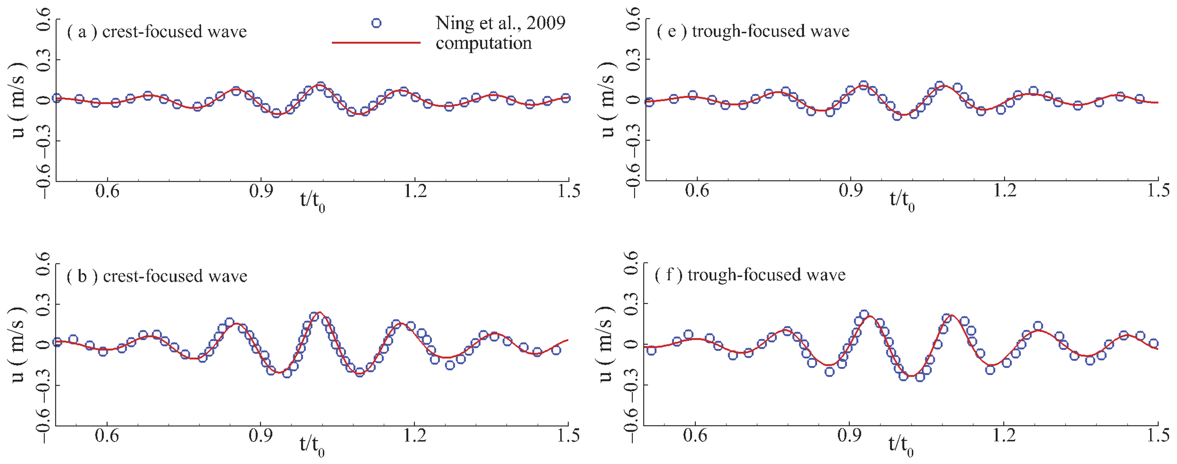
4.1. Propagation of Focused Wave
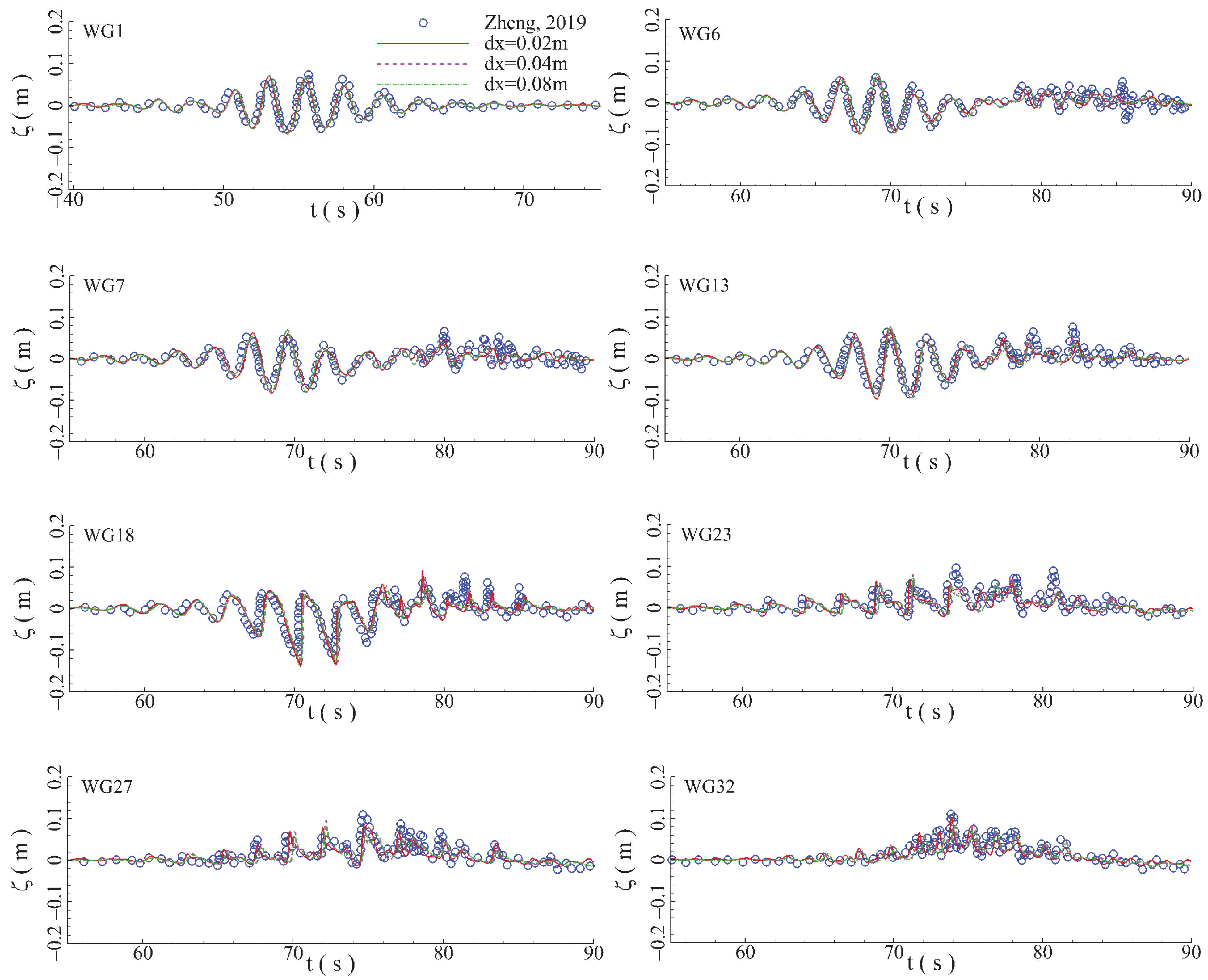
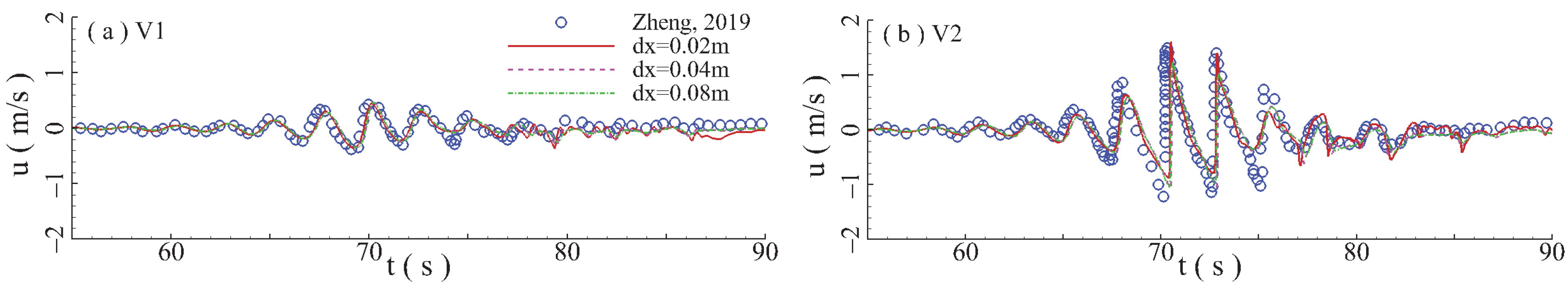
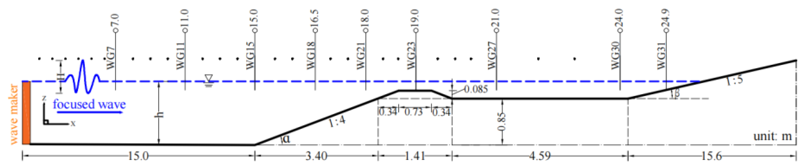
4.2. Transformation of Focused Wave Group on Fringing Reef
5. Results and Discussion
5.1. Complex Flow Phenomena
5.2. Influences of Significant Wave Height
5.3. Influences of Peak Wave Period
5.4. Influences of Water Depth
5.5. Influences of Reef Slopes
5.6. Influences of Ridge Width
6. Conclusions
- (1)
- By comparing the computational results with the experimental data, it can be seen that the nonhydrostatic numerical wave model (NHWAVE) can not only accurately simulate the generation and propagation of focused waves, but also accurately resolve the transformation and breaking processes of focused waves on the fringing reef. Since the NHWAVE solves the governing equations of incompressible flow without the hydrostatic assumption, it can accurately predict the temporal evolutions of water elevation and the velocity distributions with high accuracy.
- (2)
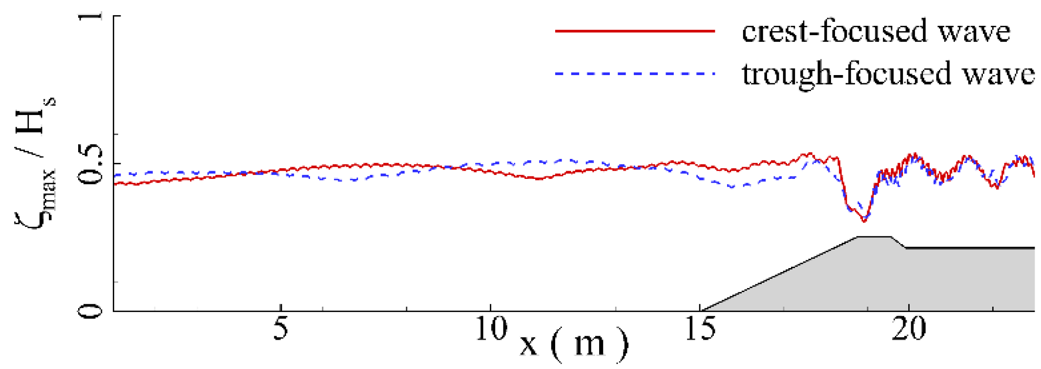
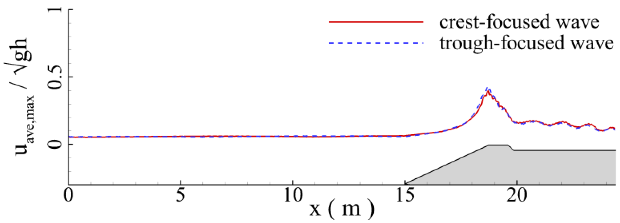
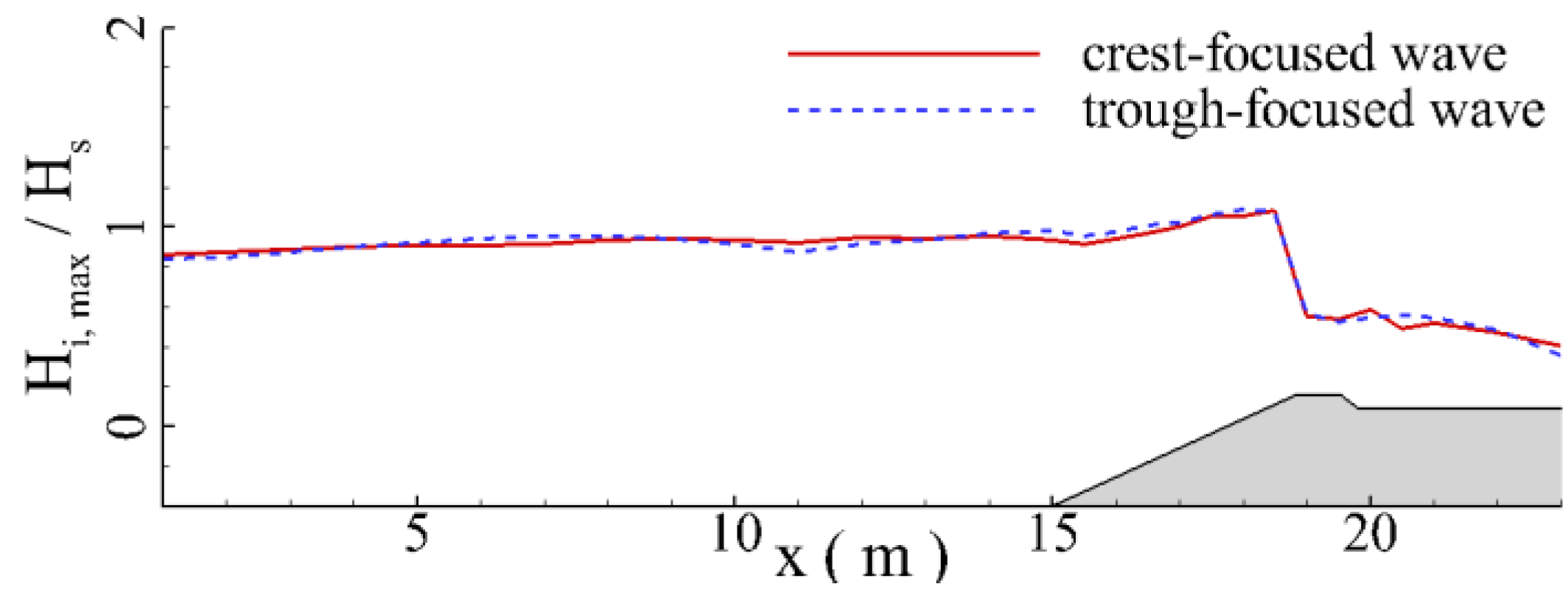
- The focused wave group undergoes complicated transformations on the fringing reef. Wave breakings of high intensity can be seen at the reef crest. The local wave heights can be effectively decreased through the wave breakings and bottom frictions. Meanwhile, strong wave reflections can be observed at the forereef and backreef slopes and the reef crest. Most of the wave energy can be lost through the complex wave hydrodynamics of focused waves on the fringing reef (about 87.8%). Meanwhile, there exist very limited differences between the wave hydrodynamics of crest-focused wave and trough-focused wave on the fringing reef.
- (3)
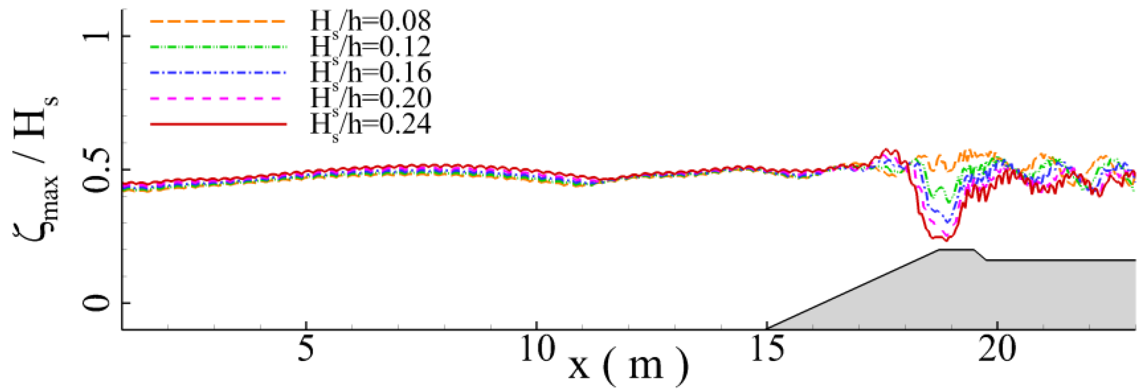
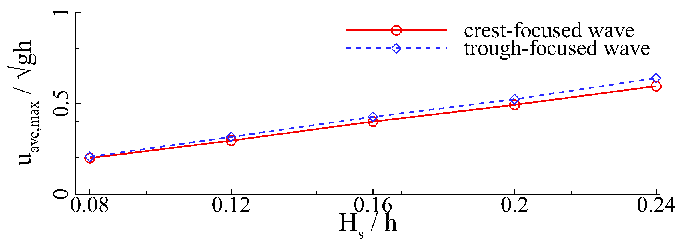
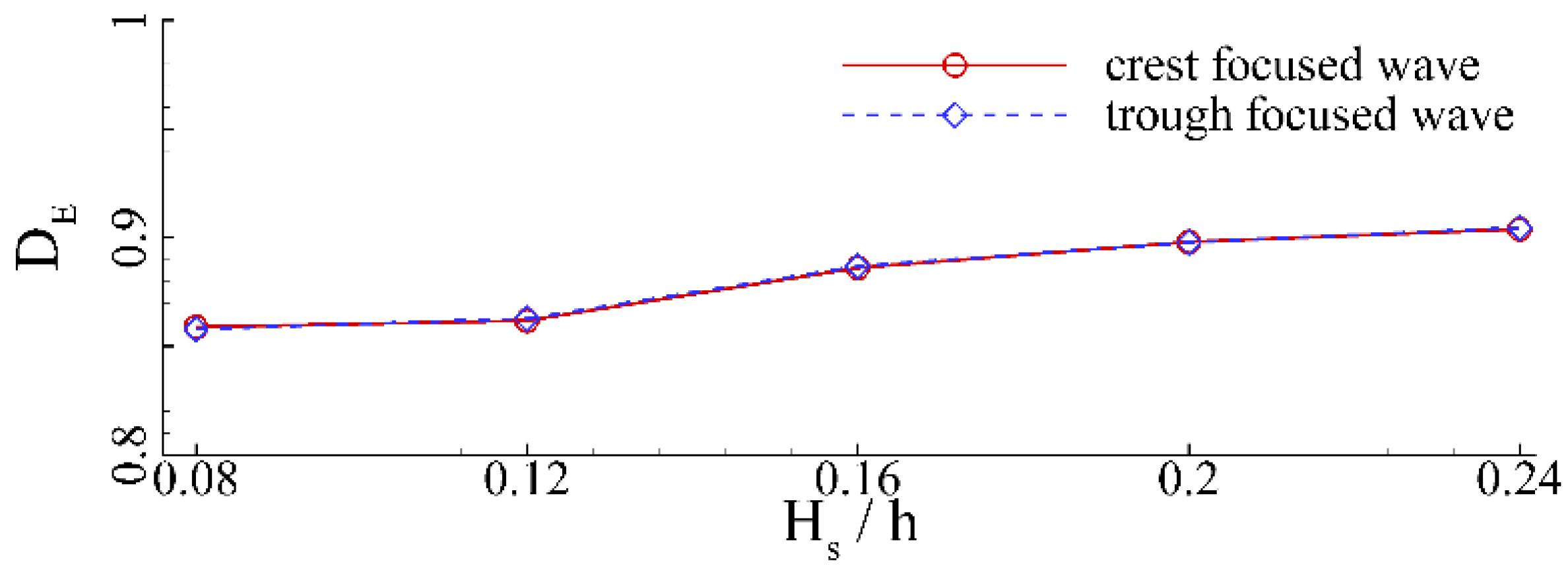
- As the significant wave height gradually increases, relative local maximum wave height decreases more due to the wave breaking process at the reef crest. Nevertheless, wave energy dissipation rate increases slightly with the significant wave height. The wave energy dissipation rate can be increased by 5.3%. Maximum wave runup heights of the crest-focused wave and the trough-focused wave can be increased by 64.7% and 62.5%, respectively, as the relative significant wave height gradually increases from 0.08 to 0.24.
- (4)
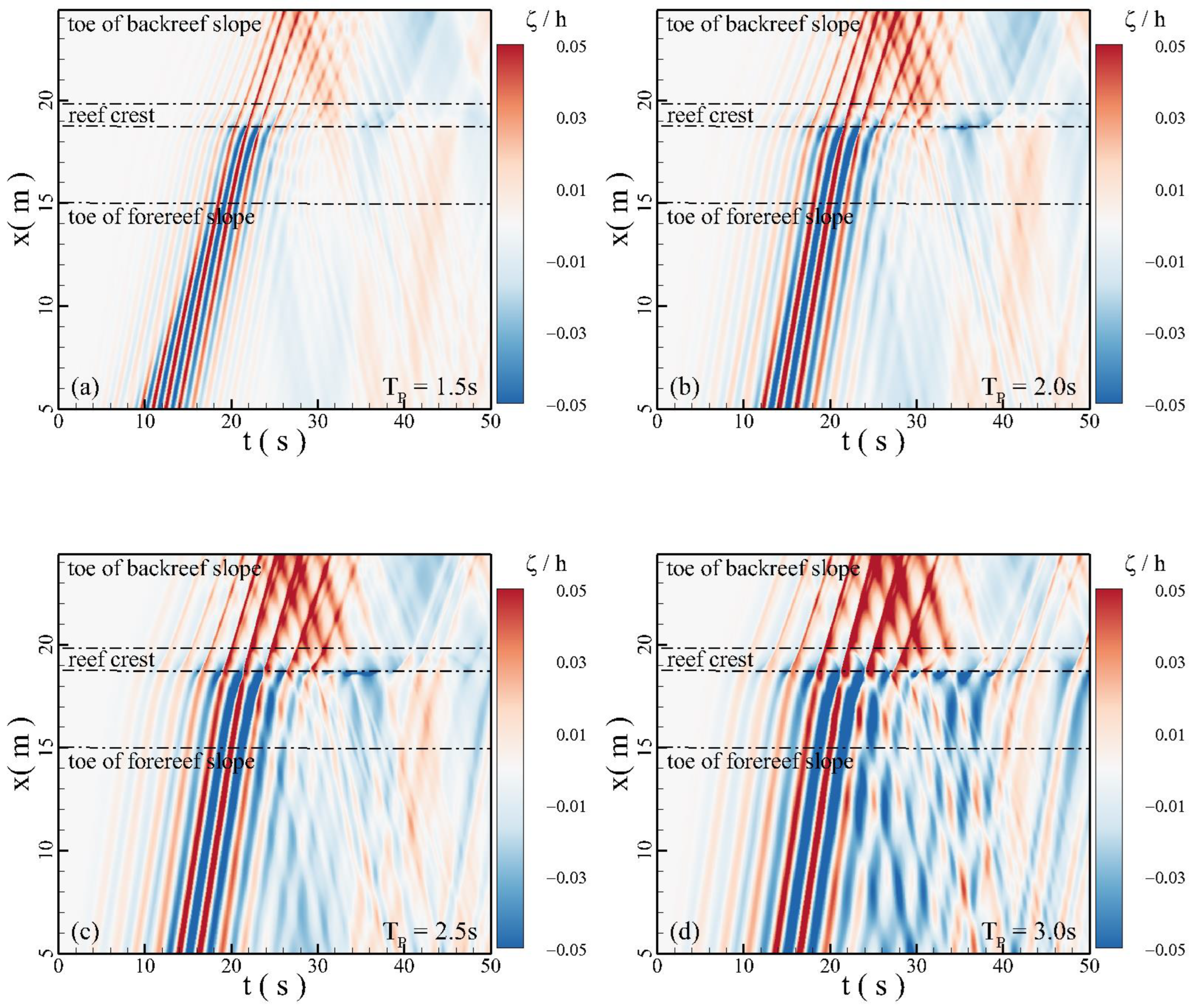
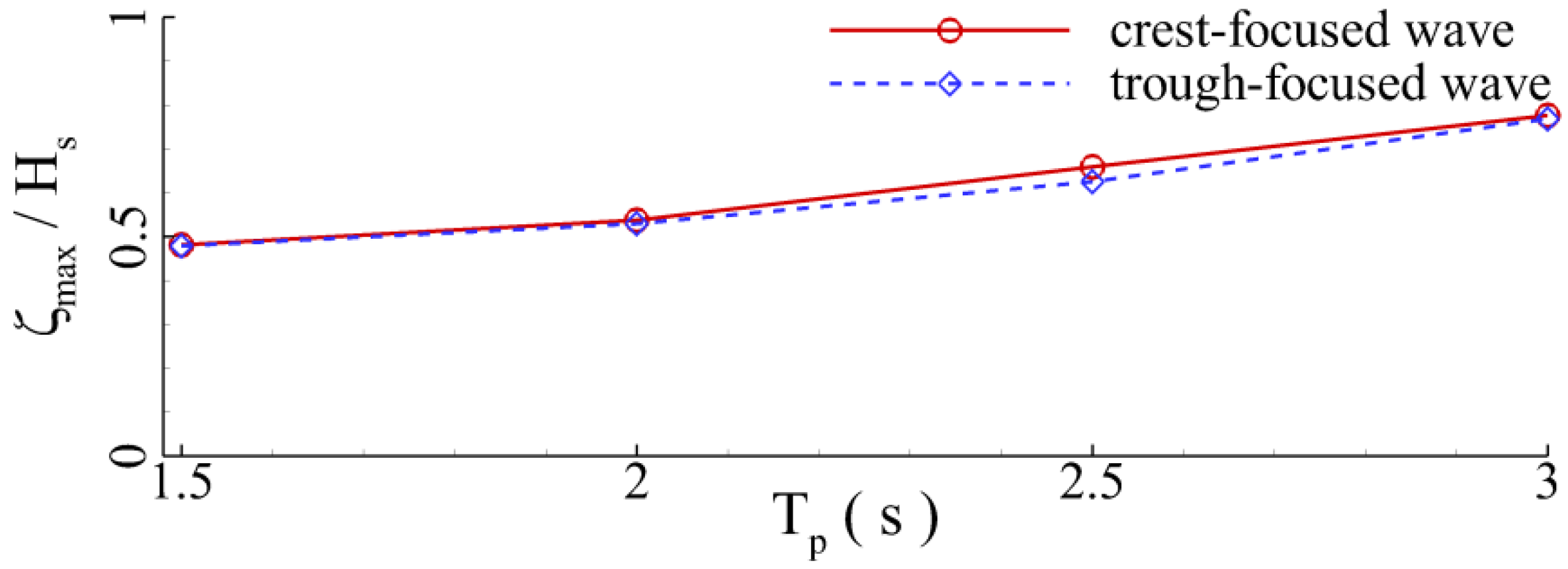
- The intensity of wave reflections at the forereef slope, as well as that at the backreef slope and the reef crest, can be greatly enhanced with the peak wave period. Although wave energy dissipation rate is slightly affected by the variation of peak wave period, wave breaking point can be noticeably affected. The maximum wave runup heights of the crest- and trough-focused waves can be increased by 55.6% and 61.1%, respectively, as the peak wave period increases from 1.5 s to 3 s.
- (5)
- When the reef crest is dry, the maximum local wave height exhibits an oscillation behavior before the occurrence of the wave breakings at the reef crest. When the submergence water depth is large enough at the reef flat, the maximum local wave height does not decrease significantly after wave breakings at the reef crest. The maximum wave runup height monotonically increases with water depth.
- (6)
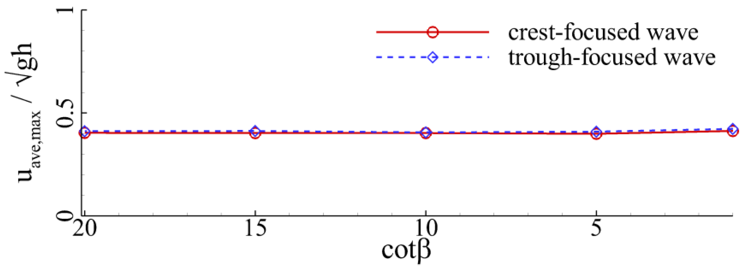
- When the forereef slope is steep, intensity of the wave reflections at the forereef slope is relatively strong. Since the intensity of wave reflection increases with the forereef slope, breaking-induced velocity over the forereef slope and reef crest tends to decrease. Nevertheless, influences of the variation of forereef slope on wave energy dissipation rate and maximum wave runup height are negligible.
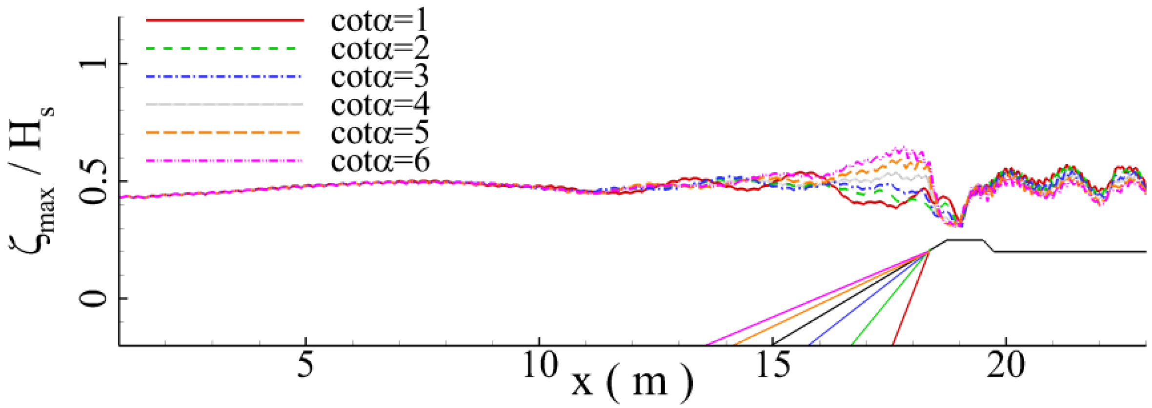
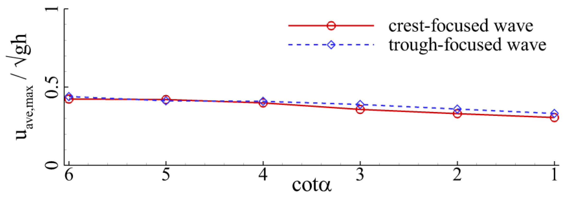
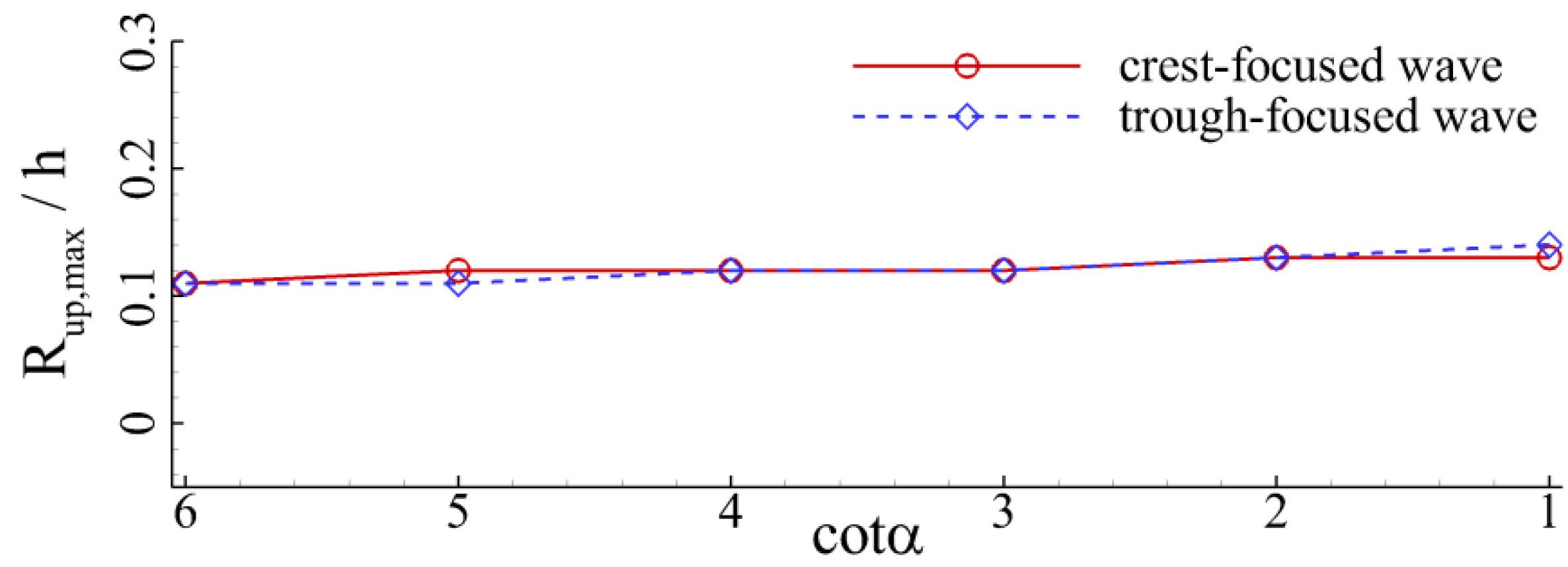
- (7)
- When the backreef slope gradually increases from = 20 to = 1, maximum wave runup height of the trough-focused wave group increases by 53.3%. Although the maximum wave runup height of crest-focused wave group also increases from = 20 to = 5, and maximum wave runup height of crest-focused wave group tends to decrease with the backreef slope if < 5. It is possibly attributed to the fact that when the backreef slope is = 1, there exist strong wave reflections, and the superposition of reflected waves and incident waves inhibits the wave runup height to a certain extent.
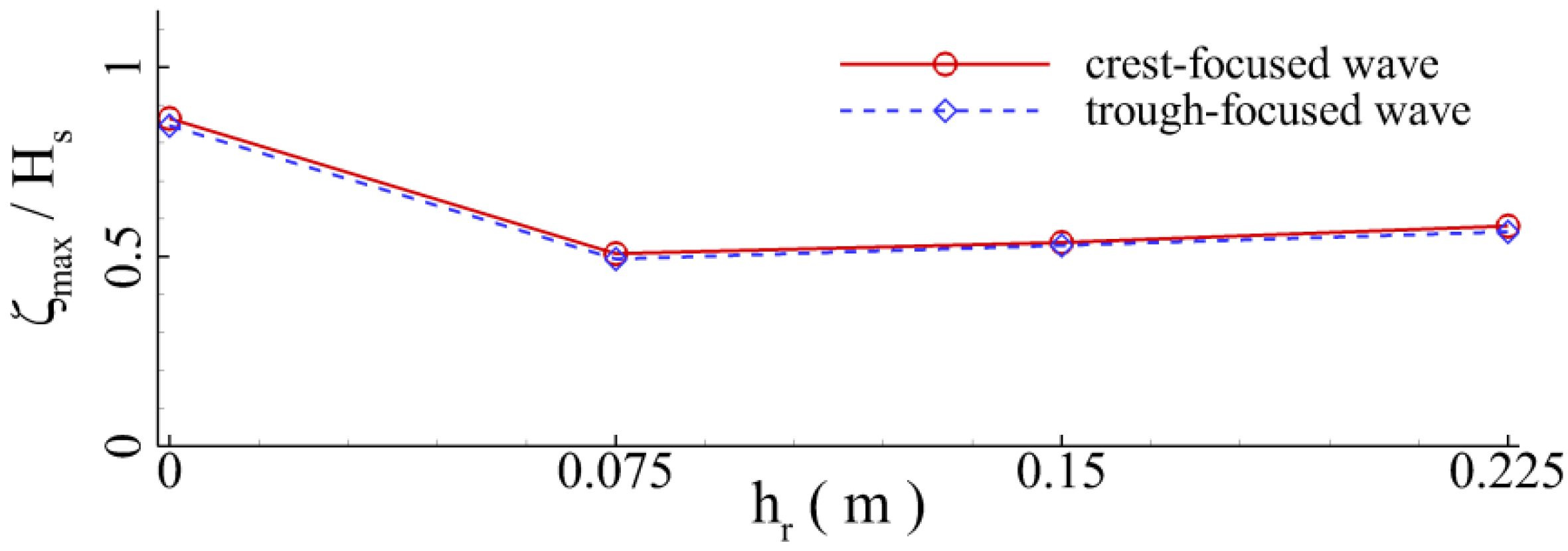
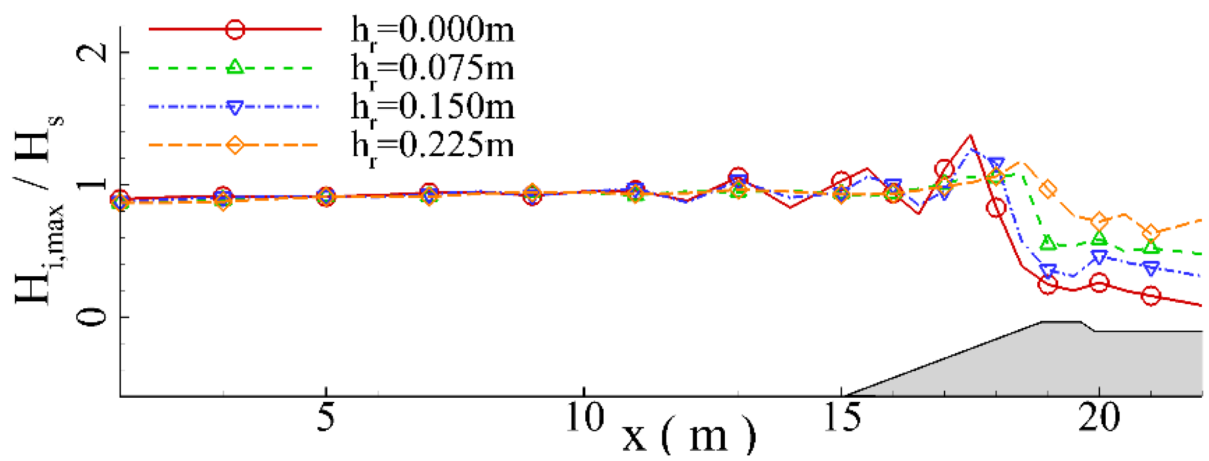
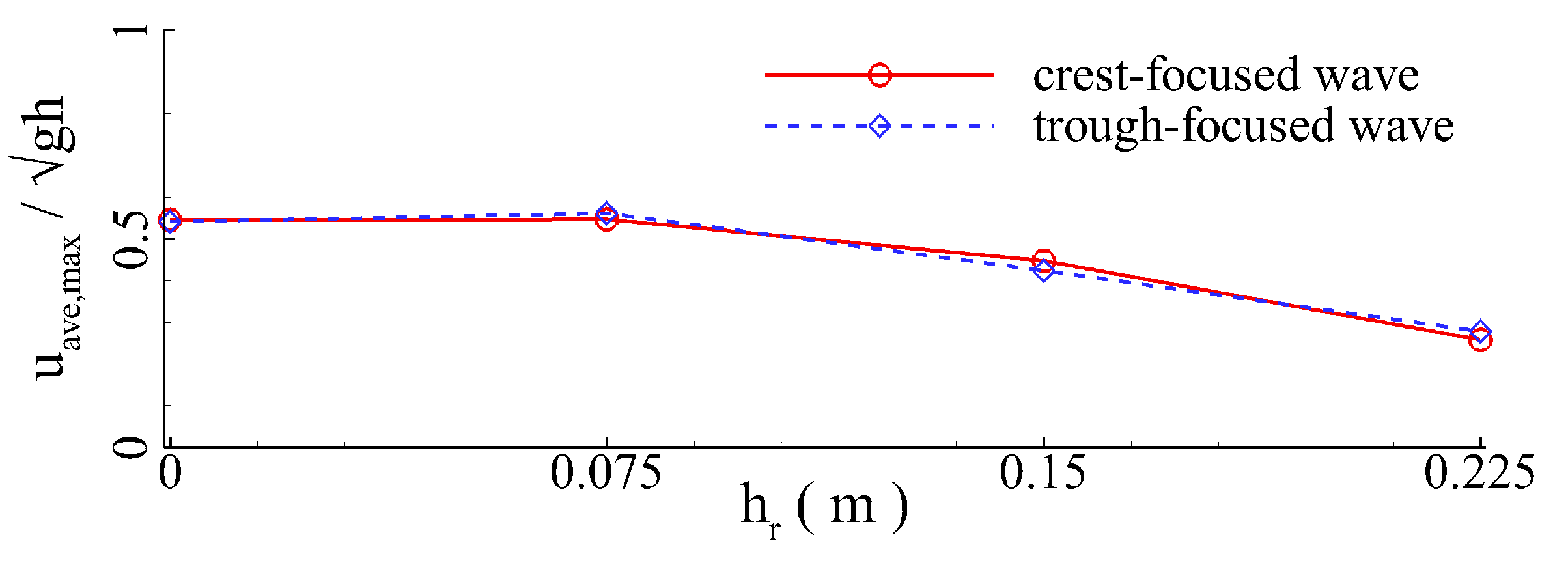
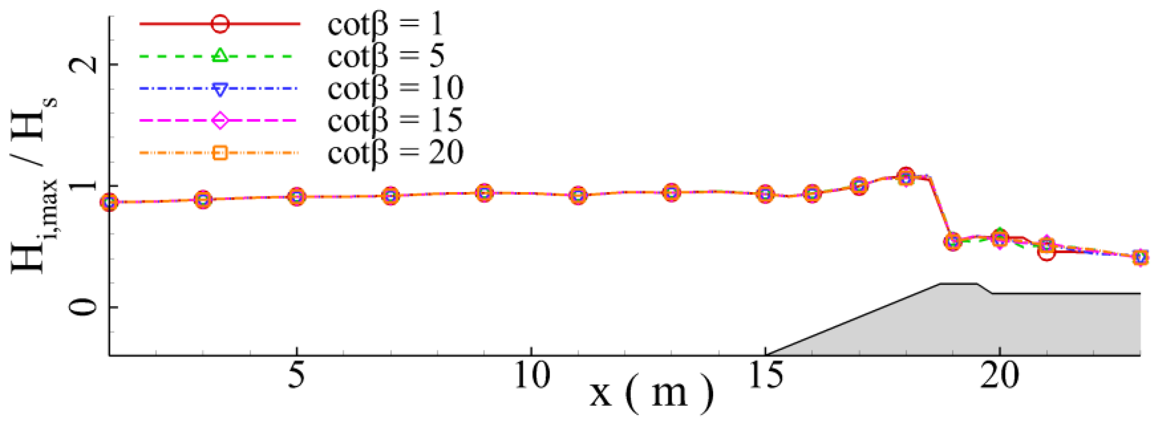
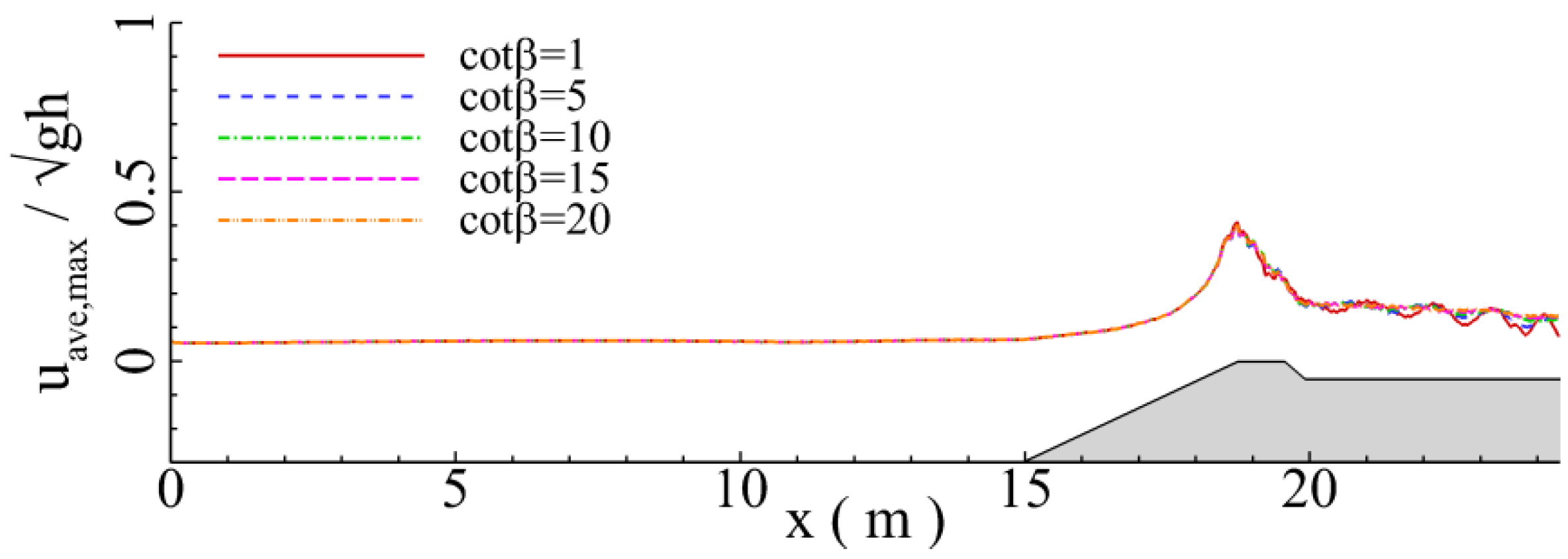
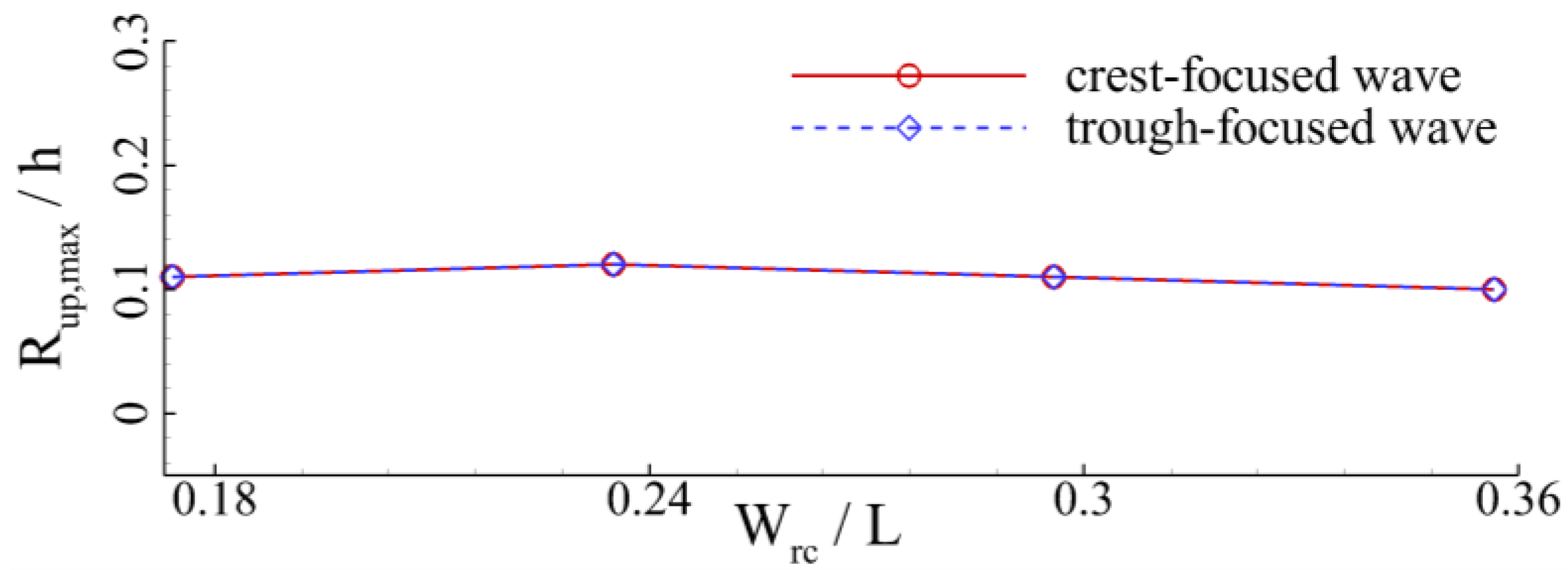
- (8)
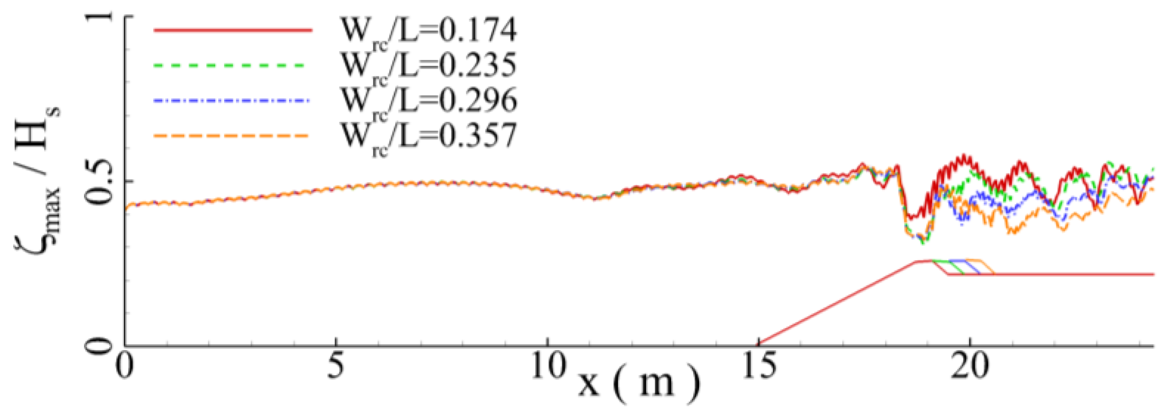
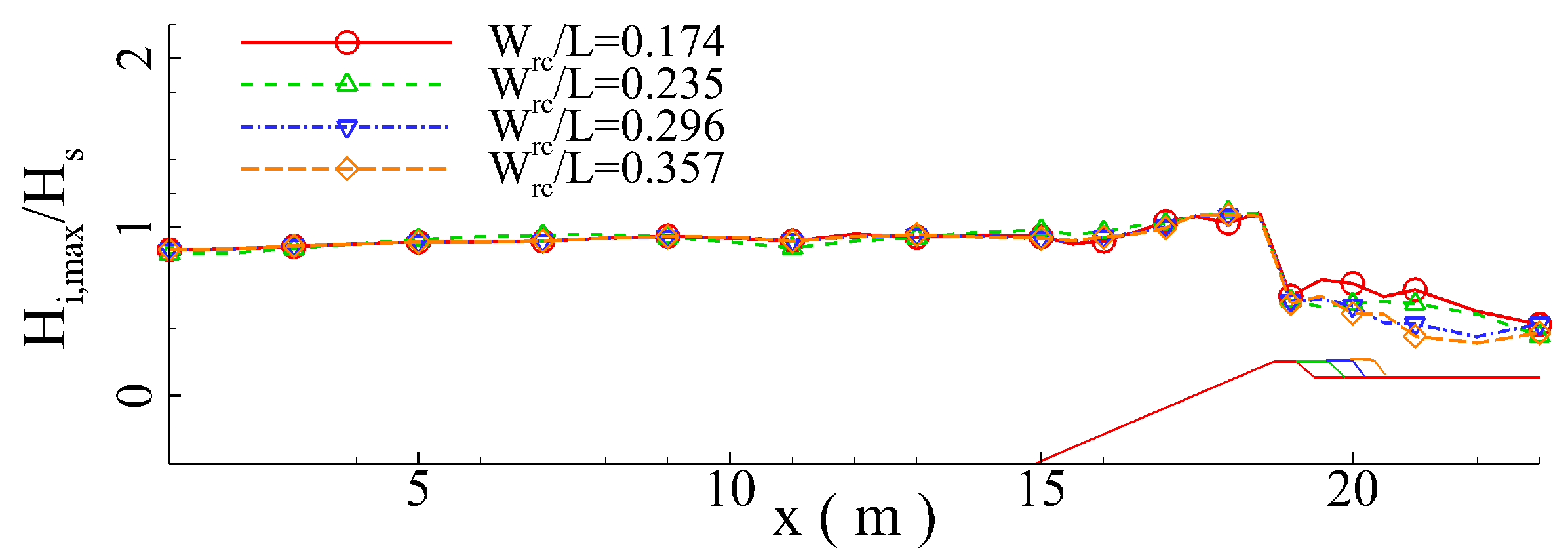
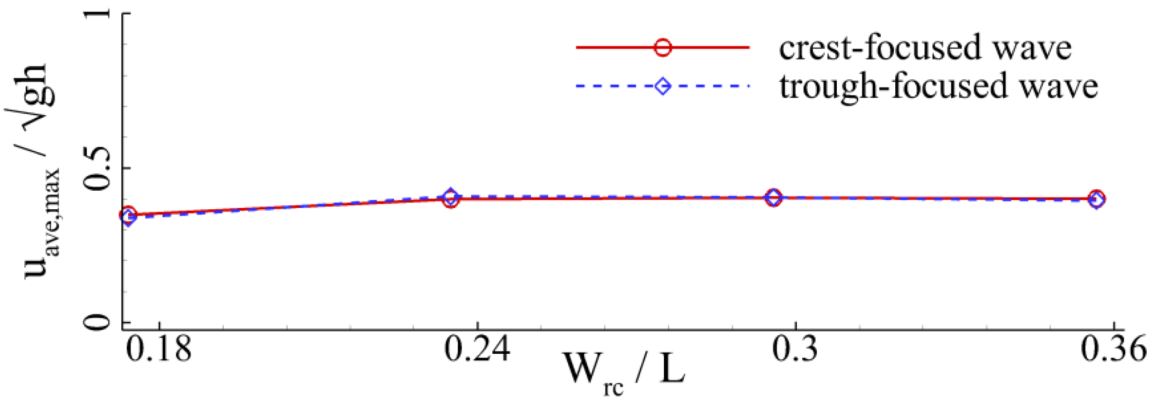
- Wave breakings can be gradually intensified with the ridge width. The maximum local wave height tends to gradually decrease with ridge width after wave breaking point. It is possibly attributed to the fact that the acting period and intensity of the bottom friction at the high-speed water column above the reef crest tend to increase with the ridge width, which finally causes maximum local wave height to decrease. The maximum wave runup height approaches its peak value at when the = 0.235.
Author Contributions
Funding
Institutional Review Board Statement
Informed Consent Statement
Data Availability Statement
Conflicts of Interest
References
- Synolakis, C.E.; Bernard, E.N. Tsunami science before and beyond Boxing Day 2004. Philos. Trans. R. Soc. A 2006, 364, 2231–2265. [Google Scholar] [CrossRef]
- Mori, N.; Takahashi, T. The 2011 Tohoku Earthquake Tsunami Joint Survey Group (2012) Nationwide post event survey and analysis of the 2011 Tohoku earthquake tsunami. Coast. Eng. 2012, 54, 1–27. [Google Scholar]
- Nikolkina, I.; Didenkulova, I. Rogue waves in 2006–2010. Nat. Hazards Earth Syst. Sci. 2011, 11, 2913–2924. [Google Scholar] [CrossRef]
- Gourlay, M.R. Wave set-up on coral reefs. 2. Set-up on reefs with various profiles. Coast. Eng. 1996, 28, 17–55. [Google Scholar] [CrossRef]
- Yao, Y.; Zhang, Q.; Becker, J.M.; Merrifield, M.A. Boussinesq modeling of wave processes in field fringing reef environments. Appl. Ocean Res. 2020, 95, 102025. [Google Scholar] [CrossRef]
- Hardy, T.A.; Young, I.R. Field study of wave attenuation on an offshore coral reef. J. Geophys. Res.-Oceans 1996, 101, 14311–14326. [Google Scholar] [CrossRef]
- Gelfenbaum, G.; Apotsos, A.; Stevens, A.W.; Jaffe, B. Effects of fringing reefs on tsunami inundation: American Samoa. Earth-Sci. Rev. 2011, 107, 12–22. [Google Scholar] [CrossRef]
- Langodan, S.; Antony, C.; Shanas, P.R.; Dasari, H.P.; Abualnaja, Y.; Knio, O.; Hoteit, I. Wave modeling of a reef-sheltered coastal zone in the Red Sea. Ocean Eng. 2020, 207, 107378. [Google Scholar] [CrossRef]
- Fang, K.; Xiao, L.; Liu, Z.; Sun, J.; Dong, P.; Wu, H. Experiment and RANS modeling of solitary wave impact on a vertical wall mounted on a reef flat. Ocean Eng. 2022, 244, 110384. [Google Scholar] [CrossRef]
- Sous, D.; Tissier, M.; Rey, V.; Touboul, J.; Bouchette, F.; Devenon, J.L.; Chevalier, C.; Aucan, J. Wave transformation over a barrier reef. Cont. Shel. Res. 2019, 184, 66–80. [Google Scholar] [CrossRef]
- Mandlier, P.G.; Kench, P.S. Analytical modelling of wave refraction and convergence on coral reef platforms: Implications for island formation and stability. Geomorphology 2012, 159, 84–92. [Google Scholar] [CrossRef]
- de Almeida, J.L.; Martinho, M.S. Experimental evaluation of the shore protection potential of the novel REEFS wave energy converter. Ocean Eng. 2020, 217, 107918. [Google Scholar] [CrossRef]
- Harris, D.L.; Vila-Concejo, A.; Webster, J.M.; Power, H.E. Spatial variations in wave transformation and sediment entrainment on a coral reef sand apron. Mar. Geol. 2015, 363, 220–229. [Google Scholar] [CrossRef]
- Gao, J.; Ma, X.; Dong, G.; Zang, J.; Ma, Y.; Zhou, L. Effects of offshore fringing reefs on the transient harbor resonance excited by solitary waves. Ocean Eng. 2019, 190, 106422. [Google Scholar] [CrossRef]
- Qu, K.; Huang, J.X.; Guo, L.; Li, X.H. Numerical Study on Hydrodynamics of Submerged Permeable Breakwater under Impacts of Focused Wave Groups Using a Nonhydrostatic Wave Model. J. Mar. Sci. Eng. 2022, 10, 1618. [Google Scholar] [CrossRef]
- Liu, J.; Bao, X.; Wang, D.; Wang, P. Seismic response analysis of the reef-seawater system under incident SV wave. Ocean Eng. 2019, 180, 199–210. [Google Scholar] [CrossRef]
- Chen, S.; Yao, Y.; Guo, H.; Jia, M. Numerical investigation of monochromatic wave interaction with a vertical seawall located on a reef flat. Ocean Eng. 2020, 214, 107847. [Google Scholar] [CrossRef]
- Ning, Y.; Liu, W.; Zhao, X.; Zhang, Y.; Sun, Z. Study of irregular wave run-up over fringing reefs based on a shock-capturing Boussinesq model. Appl. Ocean Res. 2019, 84, 216–224. [Google Scholar] [CrossRef]
- Chen, H.; Jiang, D.; Tang, X.; Mao, H. Evolution of irregular wave shape over a fringing reef flat. Ocean Eng. 2019, 192, 106544. [Google Scholar] [CrossRef]
- Liu, W.; Liu, Y.; Zhao, X.; Ning, Y. Numerical study of irregular wave propagation over sinusoidal bars on the reef flat. Appl. Ocean Res. 2022, 121, 103114. [Google Scholar] [CrossRef]
- Kench, P.S.; Brander, R.W.; Parnell, K.E.; O’Callaghan, J.M. Seasonal variations in wave characteristics around a coral reef island, South Maalhosmadulu atoll, Maldives. Mar. Geol. 2009, 262, 116–129. [Google Scholar] [CrossRef]
- Duce, S.; Vila-Concejo, A.; McCarroll, R.J.; Yiu, B.; Perris, L.A.; Webster, J.M. Field measurements show rough fore reefs with spurs and grooves can dissipate more wave energy than the reef crest. Geomorphology 2022, 413, 108365. [Google Scholar] [CrossRef]
- Liu, X.L.; Cai, Z.W.; Sun, Z.; Chen, W.W.; Jun, Y.; Ding, J.; Ye, Y.L. Study on long-term distribution and short-term characteristics of the waves near islands and reefs in the SCS based on observation. Ocean Eng. 2020, 218, 108171. [Google Scholar]
- Mann, T.; Bayliss-Smith, T.; Westphal, H. A geomorphic interpretation of shoreline change rates on reef islands. J. Coast. Res. 2016, 32, 500–507. [Google Scholar] [CrossRef]
- Smithers, S.G.; Hoeke, R.K. Geomorphological impacts of high-latitude storm waves on low-latitude reef islands—Observations of the December 2008 event on Nukutoa, Takuu, Papua New Guinea. Geomorphology 2014, 222, 106–121. [Google Scholar] [CrossRef]
- Gourlay, M.R.; Colleter, G. Wave-generated flow on coral reefs—An analysis for two-dimensional horizontal reef-tops with steep faces. Coast. Eng. 2005, 52, 353–387. [Google Scholar] [CrossRef]
- Bao, X.; Liu, J.; Li, S.; Wang, F.; Wang, P. Seismic response analysis of the reef-seawater system under obliquely incident P and SV waves. Ocean Eng. 2020, 200, 107021. [Google Scholar] [CrossRef]
- Liu, Y.; Li, S.; Liao, Z.; Liu, K. Physical and numerical modeling of random wave transformation and overtopping on reef topography. Ocean Eng. 2021, 220, 108390. [Google Scholar] [CrossRef]
- Astorga-Moar, A.; Baldock, T.E. Assessment and optimisation of runup formulae for beaches fronted by fringing reefs based on physical experiments. Coast. Eng. 2022, 176, 104163. [Google Scholar] [CrossRef]
- Kim, T.; Kwon, Y.; Lee, J.; Lee, E.; Kwon, S. Wave attenuation prediction of artificial coral reef using machine-learning integrated with hydraulic experiment. Ocean Eng. 2022, 248, 110324. [Google Scholar] [CrossRef]
- Su, S.F.; Ma, G.; Hsu, T.W. Numerical modeling of low-frequency waves on a reef island in the South China Sea during typhoon events. Coast. Eng. 2021, 169, 103979. [Google Scholar] [CrossRef]
- Guérin, T.; Bertin, X.; Coulombier, T.; de Bakker, A. Impacts of wave-induced circulation in the surf zone on wave setup. Ocean Model. 2018, 123, 86–97. [Google Scholar] [CrossRef]
- Semedo, A.; Vettor, R.; Breivik, Ø.; Sterl, A.; Reistad, M.; Soares, C.G.; Lima, D. The wind sea and swell waves climate in the Nordic seas. Ocean Dyn. 2015, 65, 223–240. [Google Scholar] [CrossRef]
- Ma, G.; Su, S.F.; Liu, S.; Chu, J.C. Numerical simulation of infragravity waves in fringing reefs using a shock-capturing non-hydrostatic model. Ocean Eng. 2014, 85, 54–64. [Google Scholar] [CrossRef]
- Nwogu, O.; Demirbilek, Z. Infragravity wave motions and runup over shallow fringing reefs. J. Waterw. Port Coast. Ocean Eng. 2010, 136, 295–305. [Google Scholar]
- Su, S.F.; Ma, G. Modeling two-dimensional infragravity motions on a fringing reef. Ocean Eng. 2018, 153, 256–267. [Google Scholar] [CrossRef]
- Su, S.F.; Ma, G.; Hsu, T.W. Boussinesq modeling of spatial variability of infragravity waves on fringing reefs. Ocean Eng. 2015, 101, 78–92. [Google Scholar] [CrossRef]
- Mase, H. Random wave runup height on gentle slope. J. Waterw. Port Coast. Ocean Eng. 1989, 115, 649–661. [Google Scholar] [CrossRef]
- Ye, J.; Shan, J.; Zhou, H.; Yan, N. Numerical modelling of the wave interaction with revetment breakwater built on reclaimed coral reef islands in the South China Sea—Experimental verification. Ocean Eng. 2021, 235, 109325. [Google Scholar] [CrossRef]
- Ford, M.R.; Becker, J.M.; Merrifield, M.A. Reef flat wave processes and excavation pits: Observations and implications for Majuro Atoll, Marshall Islands. J. Coast. Res. 2013, 29, 545–554. [Google Scholar] [CrossRef]
- Hsiao, S.C.; Lin, T.C. Tsunami-like solitary waves impinging and overtopping an impermeable seawall: Experiment and RANS modeling. Coast. Eng. 2010, 57, 1–18. [Google Scholar] [CrossRef]
- Zhu, G.; Ren, B.; Wen, H.; Wang, Y.; Wang, C. Analytical and experimental study of wave setup over permeable coral reef. Appl. Ocean Res. 2019, 90, 101859. [Google Scholar] [CrossRef]
- Qu, K.; Liu, T.W.; Chen, L.; Yao, Y.; Kraatz, S.; Huang, J.X.; Jiang, C.B. Study on transformation and runup processes of tsunami-like wave over permeable fringing reef using a nonhydrostatic numerical wave model. Ocean Eng. 2022, 243, 110228. [Google Scholar] [CrossRef]
- Guo, L.; Qu, K.; Huang, J.X.; Li, X.H. Numerical study of influences of onshore wind on hydrodynamic processes of solitary wave over fringing reef. J. Mar. Sci. Eng. 2022, 10, 1645. [Google Scholar] [CrossRef]
- Whittaker, C.N.; Fitzgerald, C.J.; Raby, A.C.; Taylor, P.H.; Orszaghova, J.; Borthwick, A.G.L. Optimisation of focused wave group runup on a plane beach. Coast. Eng. 2017, 121, 44–55. [Google Scholar] [CrossRef]
- Qu, K.; Lan, G.Y.; Sun, W.Y.; Jiang, C.B.; Yao, Y.; Wen, B.H.; Liu, T.W. Numerical study on wave attenuation of extreme waves by emergent rigid vegetation patch. Ocean Eng. 2021, 239, 109865. [Google Scholar] [CrossRef]
- Qu, K.; Sun, W.Y.; Ren, X.Y.; Kraatz, S.; Jiang, C.B. Numerical investigation on the hydrodynamic characteristics of coastal bridge decks under the impact of extreme waves. J. Coast. Res. 2021, 37, 442–455. [Google Scholar] [CrossRef]
- Zheng, Z.Y. The Study of Hydrodynamic Characteristics of Focusing Wave Propagating over a Typical Reef Island. Master’s Thesis, Dalian University of Technology, Dalian, China, 2019. [Google Scholar]
- Fan, H.X.; Fang, K.Z.; Sun, J.W.; Liu, Z.B.; Wu, H. Laboratory study of focused wave propagation over fringing reef. Chin. J. Hydrodyn. 2021, 36, 532–539. [Google Scholar]
- Ma, G.; Shi, F.; Kirby, J.T. Shock-capturing non-hydrostatic model for fully dispersive surface wave processes. Ocean Model. 2012, 43, 22–35. [Google Scholar] [CrossRef]
- Ma, G.; Kirby, J.T.; Shi, F. Numerical simulation of tsunami waves generated by deformable submarine landslides. Ocean Model. 2013, 69, 146–165. [Google Scholar] [CrossRef]
- Lin, P.; Liu, P.L.F. Turbulence transport, vorticity dynamics, and solute mixing under plunging breaking waves in surf zone. J. Geophys. Res. Oceans 1998, 103, 15677–15694. [Google Scholar] [CrossRef]
- Rodi, W. Examples of calculation methods for flow and mixing in stratified fluids. J. Geophys. Res. Oceans 1987, 92, 5305–5328. [Google Scholar] [CrossRef]
- Goda, Y. Statistical variability of sea state parameters as a function of wave spectrum. Coast. Eng. Jpn. 1988, 31, 39–52. [Google Scholar] [CrossRef]
- Schäffer, H.A. Second-order wavemaker theory for irregular waves. Ocean Eng. 1996, 23, 47–88. [Google Scholar] [CrossRef]
- Ning, D.Z.; Zang, J.; Liu, S.X.; Eatock Taylor, R.; Teng, B.; Taylor, P.H. Free-surface evolution and wave kinematics for nonlinear uni-directional focused wave groups. Ocean Eng. 2009, 36, 1226–1243. [Google Scholar] [CrossRef]


| Run | (s) | (m) |
|---|---|---|
| 1 | 1.20 | 0.0626 |
| 2 | 1.20 | 0.1246 |
| 3 | 1.25 | 0.175 |
| 4 | 1.25 | 0.2062 |
Disclaimer/Publisher’s Note: The statements, opinions and data contained in all publications are solely those of the individual author(s) and contributor(s) and not of MDPI and/or the editor(s). MDPI and/or the editor(s) disclaim responsibility for any injury to people or property resulting from any ideas, methods, instructions or products referred to in the content. |
© 2023 by the authors. Licensee MDPI, Basel, Switzerland. This article is an open access article distributed under the terms and conditions of the Creative Commons Attribution (CC BY) license (https://creativecommons.org/licenses/by/4.0/).
Share and Cite
Qu, K.; Men, J.; Wang, X.; Li, X. Numerical Investigation on Hydrodynamic Processes of Extreme Wave Groups on Fringing Reef. J. Mar. Sci. Eng. 2023, 11, 63. https://doi.org/10.3390/jmse11010063
Qu K, Men J, Wang X, Li X. Numerical Investigation on Hydrodynamic Processes of Extreme Wave Groups on Fringing Reef. Journal of Marine Science and Engineering. 2023; 11(1):63. https://doi.org/10.3390/jmse11010063
Chicago/Turabian StyleQu, Ke, Jia Men, Xu Wang, and Xiaohan Li. 2023. "Numerical Investigation on Hydrodynamic Processes of Extreme Wave Groups on Fringing Reef" Journal of Marine Science and Engineering 11, no. 1: 63. https://doi.org/10.3390/jmse11010063
APA StyleQu, K., Men, J., Wang, X., & Li, X. (2023). Numerical Investigation on Hydrodynamic Processes of Extreme Wave Groups on Fringing Reef. Journal of Marine Science and Engineering, 11(1), 63. https://doi.org/10.3390/jmse11010063