Research on Fault Early Warning of Marine Diesel Engine Based on CNN-BiGRU

Abstract

The normal operation of the marine diesel engine is of great significance to ensure the normal navigation of the ship. Predicting its operation state and judging whether the diesel engine is in the abnormal state in advance can guarantee the safe navigation of the vessel. In this paper, combining the feature extraction ability of the convolutional neural network (CNN) and the time series data prediction ability of the bidirectional gated recurrent unit (BiGRU), a marine diesel engine exhaust temperature prediction model is constructed. The results show that the mean square error (MSE) of the prediction model is 0.1156, the average absolute error (MAE) is 0.2501, and the average absolute percentage error (MAPE) is 0.0005336. Then, according to the residual distribution between the predicted value and the actual value of the model output and the standard deviation of the residual calculated by using the sliding window, we set the alarm threshold, where the upper limit of residual error is 1 and the lower limit is 1. The upper limit of the standard deviation is 0.604. Finally, we used the data set under abnormal conditions for experimental verification. The results show that the method can accurately determine the fault early warning of the marine diesel engine and provides a new reference for the health management of intelligent marine equipment.

1. Introduction

As a power output device, the diesel engine can be used not only as the main power device of the ship but also as the power output device of the ship’s power station [1]. The normal operation of the main engine can guarantee the normal power output of the ship, while the marine power generation diesel engine is an essential part of the ship’s power station, which can ensure the power supply of the ship [2]. The development of economic globalization cannot be separated from the support of the shipping industry. Ninety percent of the world economy depends on the ocean. However, the carbon emissions from shipping account for about 3% of the total global carbon emissions, of which carbon dioxide is the main emission. With the rapid development of the shipping industry, the tonnage and quantity of ships are increasing, and the emission of carbon dioxide from ship equipment is growing rapidly [3]. The operation status of a marine engine directly affects the exhaust performance of the engine. Once the diesel engine breaks down, it may cause the deterioration of the operating conditions of the diesel engine, leading to a decline in the emission performance and pollution of the marine environment. In serious cases, the diesel engine will be shut down, which will affect the normal navigation of the ship and the power supply, causing damage to the ship’s equipment and even endangering the lives of the people on board [4]. At the same time, with the development of the Internet of Things, the Internet, and automation and intelligence, the structure of marine diesel engines is becoming more complex. The components are more numerous because marine diesel engines have been operating in harsh environments for a long time, and the probability of failure is increasing [5]. The traditional diesel engine monitoring and alarm technology mainly focuses on the thermal parameters of the diesel engine, such as oil temperature, water temperature, etc. These parameters will have obvious abnormalities only when the fault deteriorates to a certain extent [6]. Therefore, traditional monitoring and alarm technology cannot directly realize early fault warnings. Relatively mature fault diagnosis technologies mostly use intelligent algorithms to learn a large number of diesel engine fault features and classify them in detail. This can enable the fault location to be realized in time after the fault occurs, which is convenient for the operation and management personnel to repair the equipment. Still, it is impossible to send an alarm prompt to relevant personnel before the fault occurs [7]. Therefore, studying the fault early warning technology of the marine diesel engine and predicting its status can detect and send out alarms at the early stage of the fault in a timely manner, which can not only give the operation management personnel enough time to check the abnormality but also save a lot of time and cost for post maintenance, which is of great significance to ensure the normal operation of the diesel engine and improve the reliability of equipment.

Exhaust gas temperature is an important thermal performance parameter for a marine diesel engine. It contains a large amount of state information about the diesel engine and reflects the combustion characteristics and dynamic characteristics of the diesel engine under operating conditions [8]. The exhaust gas temperature is used as a slowly changing parameter signal, which is less disturbed and has a strong fault indication. By monitoring and predicting the exhaust gas temperature, the health status of the marine diesel engine can be reflected in real-time [9].

In the existing research, the methods of fault early warning usually include the method based on the physical model and the data-driven method. If the model-based method is adopted, it is necessary to construct an accurate mathematical or physical model to describe the working process of the predicted object [10]. For marine equipment in harsh and changeable environments, it is often difficult to establish a more accurate model system. The data-driven method does not involve the construction of complex models. It can collect historical operation data from the equipment as the object of study [11]. By processing and analyzing the data and using relevant algorithms, we can establish a fault early warning model to realize fault early warning. In recent years, with the rapid development of deep learning and the continuous improvement and innovation of various intelligent algorithms, fault warning based on the data-driven method has attracted more and more attention [12].

Based on the improved random forest algorithm, Li et al. proposed a bus engine failure early warning model, set early warning indicators using rough set theory, and verified the proposed method through experiments [13]. Liu et al. used a combination of Bayesian and long-short-term neural networks (LSTM) to predict the status of nuclear power plant equipment. The residual value is used to set the threshold value, and the early fault warning is realized by observing the change in the residual value [14]. Zhang et al. used the multivariate state estimation technique (MSET) to establish a state prediction model for power plant auxiliary equipment and used sliding window similarity instead of the traditional residual threshold method to achieve effective fault prediction and early warning of faults [15]. Liang et al. used the bidirectional recurrent neural network (BRNN) to establish a wind turbine prediction model and calculated the residual between the predicted value and the actual value. A fault warning can be achieved by using the sliding window to calculate the residual value [16]. Yuan et al. established the echo state network (ESN) to predict the state of the pitch motor. According to the analysis of the residual value, they used the exponential weighted average algorithm to obtain the alarm threshold of each parameter to realize the early fault warning [17]. Based on the nonlinear state estimation method, Yan et al. established a gearbox bearing temperature prediction model and analyzed the distribution characteristics of the residual error and the standard deviation of the residual error through the sliding window error statistical analysis method. When the abnormal state exceeds the set threshold, a fault warning can be realized [18]. Liu et al. used the LSTM model to predict the trend of the data, which was used to predict the exhaust gas temperature of the marine diesel engine [19]. Desbazeille et al. established a neural network model for cylinder fault prediction in marine diesel engines to predict the vibration value of the crankshaft and determine the severity of the fault [20]. Cheliotis et al. combined the expected behavior (EB) model with an exponentially weighted moving average to predict the operating state of the main engine. The results show that this method can detect faults early [21]. Han et al. used the LSTM network to build a fault prediction model to predict the load of the marine diesel engine [22]. Theodoropoulos et al. used a one-dimensional convolutional neural network (Convolution1d, 1DCNN) to predict and analyze the ship data collected by sensors. The prediction results show that this method can help shipowners to save on operating costs and improve operating efficiency. At the same time, it can also ensure the normal operation of ship equipment [23].

Che et al. predicted the state of multiple variables of the aircraft system based on the LSTM neural network. They used a deep belief network to evaluate and classify the state of the aircraft system [24]. Yang et al. conducted fault diagnosis research on robots based on the deep belief network (DBN). The established model can identify the fault state of the machine and give early warning in time [25]. Karatug et al. analyzed the thermal parameters of the diesel engine through the artificial neural network (ANN), judged the real-time operation status of the diesel engine, and classified the status in detail [26]. Lazakis et al. monitored the thermal parameters of the diesel engine through fault tree analysis and fault mode response analysis to achieve fault prediction and fault location of the diesel engine [27]. Vos et al. used the combination of LSTM and a support vector machine (SVM) to detect the abnormality of the reduction gearbox [28]. Kichan et al. used principal component analysis and a neural network to monitor the vibration signals of the marine diesel engine. This method could realize early fault diagnosis [29]. Christian established a real-time anomaly monitoring system for marine diesel generators based on the long and short-term memory variational automatic encoder and multi-level Otsu threshold. The system can realize early warning and fault diagnosis [30]. Chernyi et al. studied the condition diagnosis of ladle lining by using a neural network and developed relevant software to evaluate its condition and make auxiliary decisions [31]. Theodoropoulos et al. used the two-dimensional convolutional neural network (Convolution2d, 2DCNN) to identify the abnormal state of the ship during navigation. The experimental results show that this method can effectively monitor the state of the ship’s equipment and classify it [32]. Dong et al. used the convolutional neural network to establish a multi-input model for fault diagnosis of rotating machinery and achieved good results [33].

The existing research on fault early warning can be roughly divided into two categories: state prediction and state classification [34]. Among them, the state classification method requires a large amount of early fault data input to an established model for learning, which is obviously not applicable to marine diesel engines where early fault data is difficult to collect. In addition, there is little research on the fault warning of marine diesel engines. Still, the marine diesel engine is an important piece of equipment to ensure the safe navigation of ships and the normal lives of personnel. Therefore, this paper proposes a state prediction model based on CNN-BiGRU to predict the exhaust temperature of the marine diesel engine. Then, we use the knowledge of mathematical statistics to analyze the residual value between the predicted value and the actual value, and the alarm threshold of the residual value is set. At the same time, in order to prevent the prediction value of some normal states from being greatly deviated due to the prediction model itself, the sliding window algorithm is used to calculate the standard deviation of the residual value, and the alarm threshold of the standard deviation is set. Only when the residual value and the standard deviation value exceed the threshold at the same time, will the fault warning be triggered.

The rest of the research content of this paper is as follows. The convolutional neural network and the bidirectional gated recurrent unit used in this paper are introduced in the deep learning theory section. In the section on the forecasting process, the data set collected and the data processing process are introduced. The hyperparameter selection process is described. The forecasting model is established, and the advantages of the forecasting model proposed in this paper in terms of trend prediction are verified through experiments. In the section on fault warning, the setting method of the alarm threshold is introduced. The conclusion is drawn in the conclusion section.

2. Deep Learning Theory

2.1. The Convolutional Neural Network

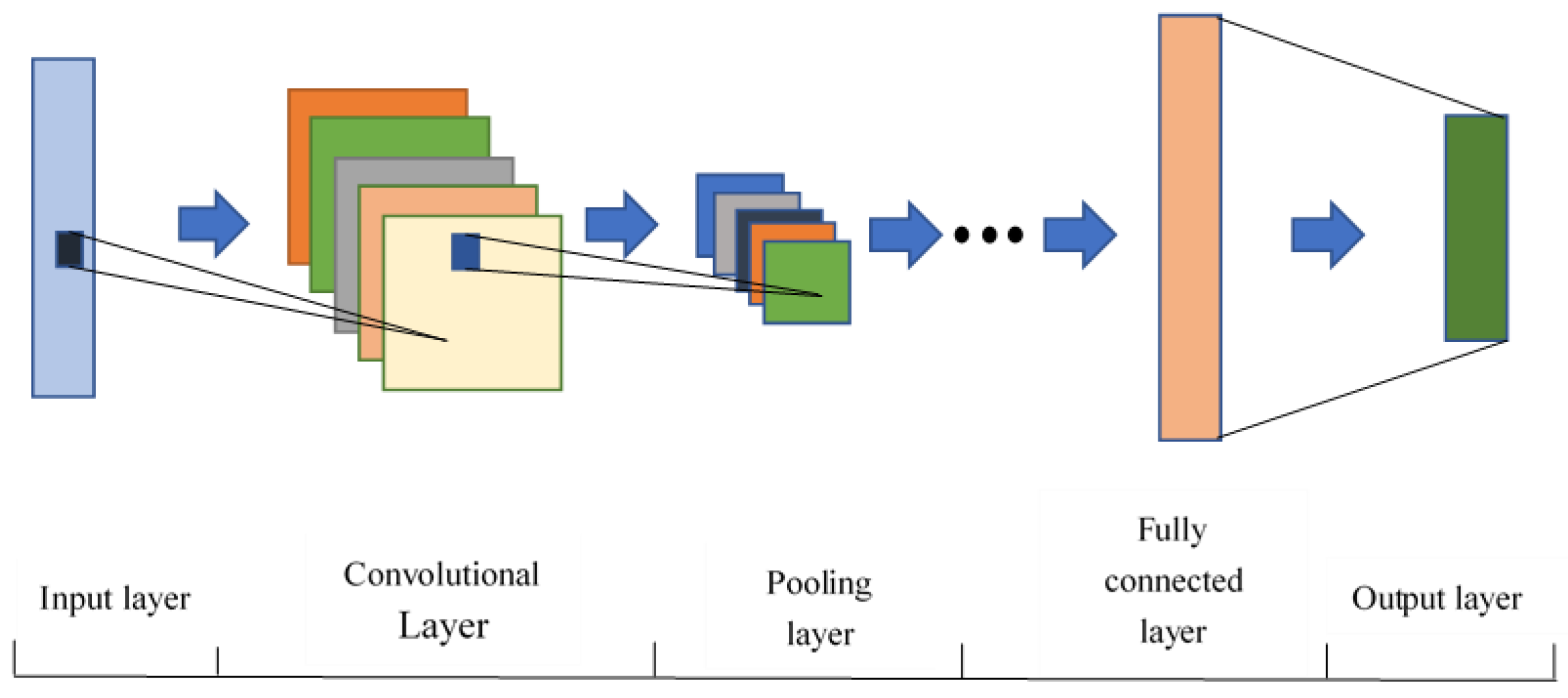
The convolutional neural network is a deep feed-forward neural network that processes network structure data and has strong feature extraction capabilities [35]. It usually consists of the input layer, the convolutional layer, the pooling layer, and the fully connected layer, and its structure diagram is shown in Figure 1 [36]. The convolution layer is named after the convolution calculation in mathematics. It realizes the convolution calculation of the input data by the convolution kernel, whose size can be adjusted. It is an essential step for CNN to realize local feature extraction. Its calculation formula is shown in the Formula (1).

$$c_t=f(W_{cnn}\ast n_t+b_{cnn})$$

(1)

In the formula, W_cnn is the weight coefficient of the convolution kernel; n_t is the input variable at time t; * represents the convolution operation; b_cnn represents the deviation coefficient of the convolution operation; c_t is the output after the convolution layer operation; f means the convolution activation function during operation.

The pooling layer is usually located after the convolutional layer. Its main function is small, based on the premise of ensuring that the feature information is not lost, reducing the amount of calculation, and avoiding the phenomenon of overfitting. Average pooling and maximum pooling are the two most commonly used pooling methods at present.

The fully connected layer will rearrange the features and perform nonlinear calculations to obtain the output results.

CNN is widely used in image processing, and its application type is the 2DCNN. Still, because its latitude does not match the time series data, it cannot be directly applied to the time series data prediction problem. To solve this problem, the 1DCNN is often used to process time-series data and mine the internal correlation and potential features of the data to improve the efficiency and accuracy of the prediction model [37].

2.2. The Bidirectional Gated Recurrent Unit

Recurrent neural networks (RNN) and their variants are widely applied in the study of time series prediction. Compared with traditional neural networks, the RNN has a certain memory ability to relate the effects produced by historical data into the current training and learning process, resulting in a relatively ideal prediction effect. Because only a single tanh unit is included in its interior, problems such as gradient disappearance and gradient explosion are easily encountered in the process of training. In response to this problem, the long-short-term neural network and the gated recurrent unit (GRU) are improved based on the RNN, which can well circumvent the dropout gradient problem and optimize the prediction effect of the model.

The LSTM consists mainly of the forget gate, the input gate, and the output gate. The main function of the forget gate is to forget redundant and invalid information. The input gate filters the input information and leaves important feature information in the data. The main function of the output gate is to pass information down. The LSTM improves the RNN by altering the internal structure of neurons and solving the gradient problem in the RNN model. However, because the internal structure is more complex, the number of activation functions and training parameters set internally increases, which increases the difficulty of training and reduces the speed of model prediction. In order to improve the prediction speed of the model on the premise of ensuring prediction accuracy, simplify its internal structure as much as possible, so some scholars proposed the GRU network.

The GRU is also a gating mechanism in the recurrent neural network, which is proposed to solve problems such as long-term memory and gradient in backpropagation [38]. The GRU is similar to the LSTM. By simplifying the internal structure of the LSTM network, an update gate is used to replace the roles of the input gate and the forgetting gate inside the network. Therefore, compared with LSTM, the GRU network has fewer parameters [39]. In the GRU network unit, the reset gate is used to integrate the previous state information with the current state information as the output of the current state information. The update gate selectively forgets the hidden state of the previous moment by obtaining the hidden state h_t−1 of the previous moment, the current input X_t and the current state information ĥ_t, and passing their combined matrix through the nonlinear change of the activation function. That is, forget some unimportant information in h_t−1 and selectively remember some information in ĥ_t. The basic structure of the GRU network unit is shown in Figure 2 [40], and the mathematical calculation formula is shown in the Formula (2).

$$\{\begin{array}{l}{r}_t=\sigma \left(W_r\cdot \left[h_{t-1},X_t\right]\right)\\ z_t=\sigma \left(W_z\cdot \left[h_{t-1},X_t\right]\right)\\ {\hat{h}}_t=\sigma \left(W_{\hat{h}}\cdot \left[r_t\times h_{t-1},X_t\right]\right)\\ h_t=\left(1-z_t\right)\times h_{t-1}+z_t\times {\hat{h}}_t\end{array}$$

(2)

In the formula, X_t, h_t−1, z_t, r_t, ĥ_t, and h_t, respectively, represent the input information at the current moment, the hidden state at the previous moment, the update gate, the reset gate, the candidate hidden state, and the output of the hidden layer at the current moment. W_r, W_z, W_ĥ is the weight parameter matrix of the GRU neural network. σ is the sigmoid function.

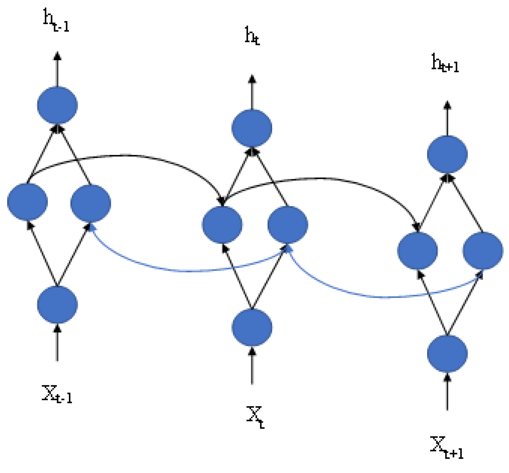
In the GRU neural network, the current state is always determined by the state at the previous moment; that is, it is output from front to back. However, in actual situations, if the feedback of a certain moment to the state of a future moment is considered, it is more conducive to the extraction of deep features, which requires BiGRU to establish this connection [41]. BiGRU is a neural network model composed of GRU cells with one-way and opposite directions, and the output is determined by the states of these GRU cells. At each moment, the input will provide two GRU cells with opposite directions simultaneously, and the output will be jointly determined by the two unidirectional GRU cells. The specific structure of BiGRU is shown in Figure 3 [42]. The output is shown in the Formula (3).

$$\{\begin{array}{l}{h}_{t1}=GRU\left(x_t,h_{t-1}\right)\\ h_{t2}=GRU\left(x_t,h_{t+1}\right)\\ ht=W\times h_{t1}+V\times h_{t2}+b_t\end{array}$$

(3)

In the formula, the GRU function represents the nonlinear transformation of the input sequence vector, turning the input at the current moment and the input at the adjacent moment into the corresponding hidden layer state; x_t is the input at time t; h_t−1 is the state of the hidden layer at time t − 1; h_{t + 1} is the state of the hidden layer at time t + 1; W, V represent the weights corresponding to the state of the forward hidden layer and the state of the reverse hidden layer, respectively, and b_t represents the bias corresponding to the state of the hidden layer at time t.

2.3. CNN-BiGRU Prediction Model

Compared with traditional neural networks, CNN can efficiently and accurately extract features from data sets. However, when dealing with long time series data, CNN cannot effectively analyze the time series features in the data, let alone accurately predict the time series data. Therefore, this paper adopts 1DCNN to convert the long time series into shorter ones composed of high-dimensional features and then outputs them to the next layer of network training through a pooling layer operation. Considering that the diesel engine exhaust temperature prediction contains the continuity principle and the correlation principle. In this paper, the exhaust temperature at the previous time and the influencing factors of the exhaust temperature at the previous time are linked with the exhaust temperature prediction. The BiGRU neural network is used to conduct two-way training on the time series, which can learn the complete information of the entire time series data and effectively extract and use the time series characteristics in the data.

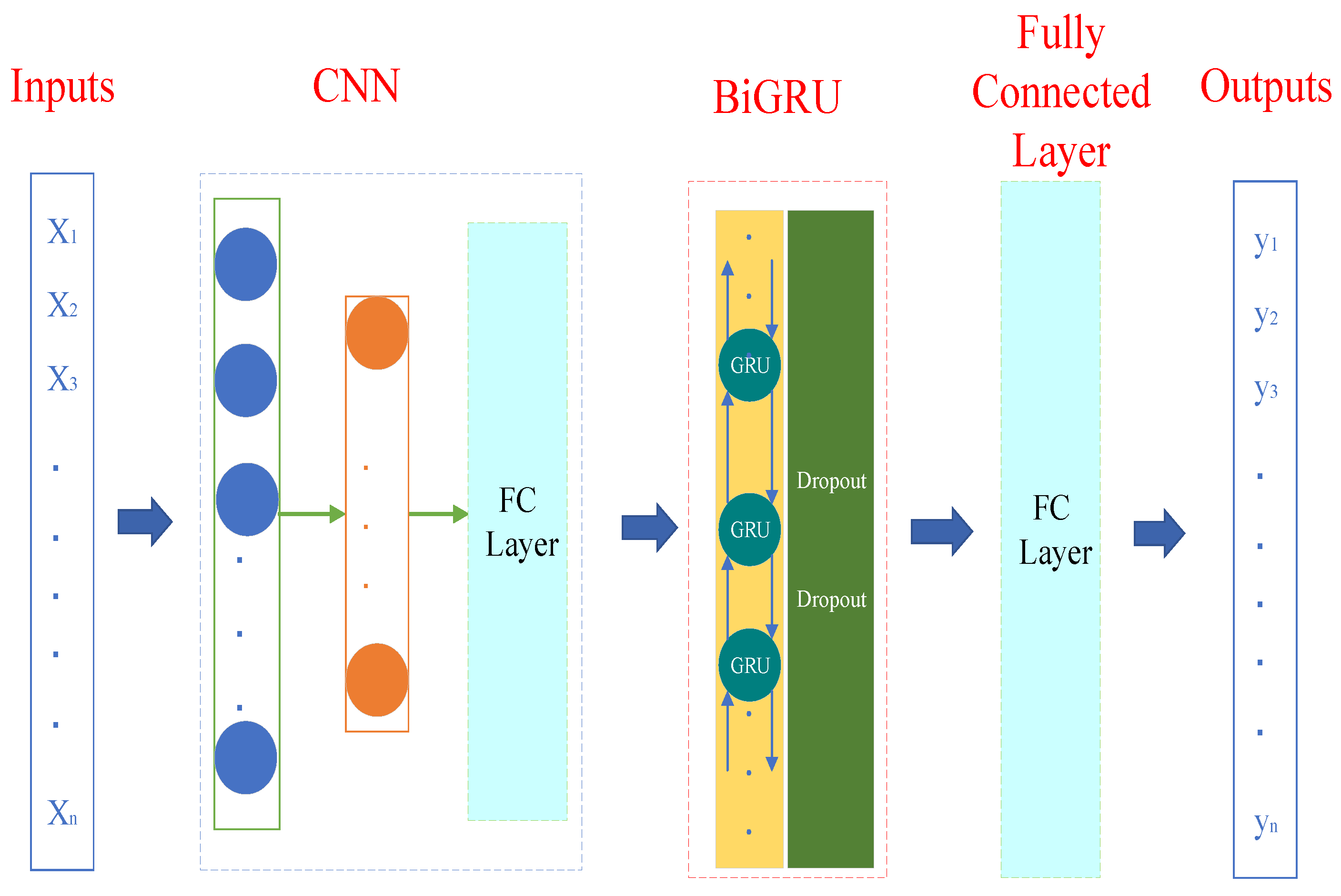
In conclusion, this paper proposes a prediction model combining the CNN and the BiGRU, which makes full use of the advantages of the CNN in feature extraction and the BiGRU in time series feature prediction, and improves the prediction accuracy of the prediction model through this combined neural network. The framework diagram of the marine diesel engine exhaust temperature prediction model is shown in Figure 4. The model is mainly divided into an input layer, a CNN layer, a BiGRU layer, a full connection layer, and an output layer. Each layer in the model is described as follows: (1) Input layer. The collected diesel engine exhaust temperature and other thermodynamic parameter data are used as the input of the prediction model, and its expression is shown in the Formula (4).

$$X=\left[\begin{array}{cccc}{x}_1{}^1& x_1{}^2& \dots & x_1{}^n\\ x_2{}^1& x_2{}^2& \dots & x_2{}^n\\ ⋮& ⋮& ⋮& ⋮\\ x_i{}^1& x_i{}^2& \dots & x_i{}^n\end{array}\right]$$

(4)

In the formula, x_iⁿ represents the value of thermal parameter i collected at time n.

(2) CNN layer. Extracting the temporal and spatial characteristics of the input diesel engine historical operation data, which is composed of a convolution layer, a pool layer and a full connection layer. Map the data processed by the convolution layer and pooling layer to the hidden layer feature space and output it after the full connection layer as the input of the BiGRU layer.

(3) BiGRU layer. Building a single-layer, two-way GRU structure, learning the data extracted from the CNN layer, fully capturing the changing rules of its internal information characteristics, and inputting them to the full connection layer. At the same time, in order to prevent the model from overfitting, Dropout is added to this layer to randomly discard some hidden layer nodes during the training process.

(4) Full connection layer. Converting the input of BiGRU into prediction results and inputting them into the output layer.

(5) Output layer. Outputting the predicted value of exhaust temperature.

3. Forecasting Process

3.1. Data Analysis and Processing

The data selected in this paper are the real-time operation data of a 6L34DF marine dual-fuel power generation diesel engine collected from an LNG electric propulsion ship. A total of 7000 monitoring points were collected, and the time interval between collection points was 5 s. There are seven types of collected data, as shown in

Table 1. Type of parameters.

Data Type	Symbol	Unit
The exhaust temperature of diesel engine	TP	°C
The load of diesel engine	L	KW
The pressure difference of lube oil filter	PC	MPa
Outlet temperature of cylinder liner water	T1	°C
Air inlet temperature	T2	°C
Speed of supercharger	N	r/min
Exhaust temperature of supercharger	T3	°C

below.

It is very important to select input variables when building a time-series data prediction model. Because this paper mainly predicts the exhaust temperature of the diesel engine, the characteristic variables with a strong correlation with exhaust temperature should be selected as far as possible in the selection of input variables to reduce the input dimension of the model and prevent the problem of overfitting the model caused by too many input dimensions.

Pearson correlation coefficients (PCCs) were proposed by Carl Pearson and are used to describe the correlation between different variables [43]. The degree of correlation between variables can be summarized by the size of the value. The formula is shown in the Formula (5).

$$r=\frac{{\displaystyle \sum _{i=1}^n\left(x_i-\overline{x}\right)\left(y_i-\overline{y}\right)}}{\sqrt{{\displaystyle \sum _{i=1}^n{\left(x_i-\overline{x}\right)}^2}}\sqrt{{\displaystyle \sum _{i=1}^n{(y_i-\overline{y})}^2}}}$$

(5)

In the formula: r indicates the degree of correlation between two variables, x and y, and the value range is between −1 and 1; $\overline{x}$ and $\overline{y}$ are respectively expressed as the average value of x_i, y_i. The correlation strength between variables is judged by the following value range: the absolute value of the correlation coefficient is 0.8~1.0, very strong correlation; 0.6~0.8, strong correlation; 0.4~0.6, moderate correlation; 0.2~0.4, weak correlation; At 0.0~0.2, there is very little or no correlation.

According to the above method, the Pearson correlation coefficient is used to analyze the correlation between various collected operating parameters and diesel engine exhaust temperature. The analysis results are shown in

Table 2. Correlation analysis of marine diesel engine operating parameters.

Data Type	TP	L	PC	T1	T2	N	T3
TP	1	0.94	0.013	0.49	−0.01	0.92	0.47
L	0.94	1	0.014	0.38	−0.011	0.94	0.39
PC	0.013	0.014	1	0.0026	−0.030	0.0061	−0.017
T1	0.49	0.38	0.0026	1	−0.11	0.30	0.39
T2	−0.01	−0.011	−0.030	−0.11	1	0.027	−0.0044
N	0.92	0.94	0.006	0.30	0.027	1	0.43
T3	0.47	0.39	−0.017	0.39	−0.0044	0.43	1

. It can be seen from Table 2 that the coefficient dimension of diesel engine load and turbocharger speed have a strong correlation with exhaust temperature. In addition, the correlation coefficient between cylinder liner water outlet temperature and exhaust gas temperature is 0.49, and the correlation coefficient between supercharger outlet exhaust gas temperature and exhaust gas temperature is 0.47. The correlation between them and exhaust temperature is moderate. Therefore, the above four operating parameters are selected as influencing factors and input into the prediction model together with the time series data of exhaust temperature to predict the subsequent exhaust temperature changes.

Since the dimensions of various parameters used as the input of the prediction model are different and vary greatly, in order to solve the negative impact caused by this problem, the maximum and minimum values of various types of data in the data set are used as reference values to normalize the data set before the input of the model. The normalization formula is shown in the Formula (6).

$$X=\frac{x-x_{\min }}{x_{\max }-x_{\min }}$$

(6)

In the formula, X is the normalized data; x is the original parameter; and x_max and x_min are the maximum and minimum values of the parameter.

3.2. Model Evaluation Index

In order to evaluate the prediction accuracy of the proposed method, MAE, MSE, and MAPE are selected as the evaluation indicators of the model prediction results. The three evaluation indicators are the calculated deviations between the predicted value and the true value. The smaller the results, the higher the prediction accuracy. The mathematical expression is shown in the Formulas (7)~(9).

$$MAE=\frac{1}{n}{\displaystyle \sum _{i=1}^n|y_i-{\widehat{y}}_i|}$$

(7)

$$MSE=\frac{1}{n}{\displaystyle \sum _{i=1}^n{\left(y_i-{\widehat{y}}_i\right)}^2}$$

(8)

$$MAPE={\displaystyle \sum _{i=1}^N\left(\left|\frac{y_i-{\widehat{y}}_i}{y_i}\right|\times \frac{1}{n}\right)}$$

(9)

where y_i represents the actual value of the exhaust temperature; ${\widehat{y}}_i$ represents the predicted value of the exhaust temperature; and n is the number of samples in the test set.

3.3. Hyperparameter Selection

To determine the hyperparameters of the BiGRU model, you need to determine the number of layers, hidden layer nodes, time step, and other parameters of the model. In this paper, the control variable method is used to optimize the structure of the BiGRU model. In the experiment to determine the number of model layers, the prediction performance is tested by increasing the number of model layers while ensuring that the CNN model parameters and other parameters of the BiGRU model remain unchanged. The experimental results of the model layers are shown in

Table 3. Prediction results of BiGRU with different numbers of network layers.

BiGRU Network Layers	MAE	MSE	MAPE
1	0.2501	0.1156	0.0005336
2	0.2634	0.1251	0.0005618
3	0.2646	0.1260	0.0005643

. The experimental results show that when the number of BiGRU layers is 1, all evaluation indexes are at their minimum, which is the optimal value. As the number of layers increases, the evaluation index value increases, indicating that the model is overlearning. We used the same method to select other parameters of the BiGRU model. After several manual debugging sessions, we set other parameters as shown in

Table 4. BiGRU network structure parameters.

Network Parameters	Setting
Hidden layer units	64
Sequence length	6
Batch size	200
Epochs	1000
Dropout	0.5
Learning Rate	0.0005
Activation Function	tanh
Optimizer	Adam
Ratio of training set to test set	7:3
Loss_function	MSEloss

.

In this paper, the CNN network used for feature extraction consists of a 1D convolutional layer and a 1D pooling layer. Based on experience and multiple manual debugging, it is determined that the number of convolution kernels is 64, the size of the convolution kernel is 3, and the activation function is ReLU. The kernel_size of the maximum pooling layer is selected to be 3, consistent with the convolution kernel size.

3.4. Result Analysis

In this work, the multi-dimensional data processed above were input into the established forecasting model. The forecasting curve is shown in Figure 5 below. It can be seen from Figure 5 that the diesel engine runs relatively smoothly during this period, and the exhaust gas temperature range basically fluctuates between 465 °C and 480 °C. The deviation between the output of the prediction model and the actual value is small, and it is basically close to the true value.

In order to verify the advantages of the prediction model proposed in this paper, the same data is input into the established RNN, LSTM, GRU, and BiGRU models. After the training of the model, the relationship between the loss and the number of training rounds can be obtained, as shown in Figure 6. It can be seen from Figure 6 that the prediction model used in this paper has the fastest convergence speed, a strong learning ability, and can learn the internal characteristics of data in a short time. After completing the training, the time required for each model to predict a step in the test process is recorded as shown in

Table 5. Comparison of time required for single step of each model.

Model	Time Required for Single Step (s)
CNN-BiGRU	0.066
BiGRU	0.33
GRU	0.39
LSTM	0.43
RNN	0.49

. It can be seen from

Table 6. Evaluation index of prediction results of different models.

Prediction Model	MAE	MSE	MAPE
RNN	0.2726	0.1463	0.0005813
LSTM	0.2675	0.1389	0.0005706
GRU	0.2592	0.1286	0.0005527
BiGRU	0.2612	0.1234	0.0005572
CNN-BiGRU	0.2501	0.1156	0.0005336

that the prediction model selected in this paper takes the shortest time to predict a step, and the prediction time is significantly reduced compared with other neural networks, highlighting the advantages of this model in prediction speed.

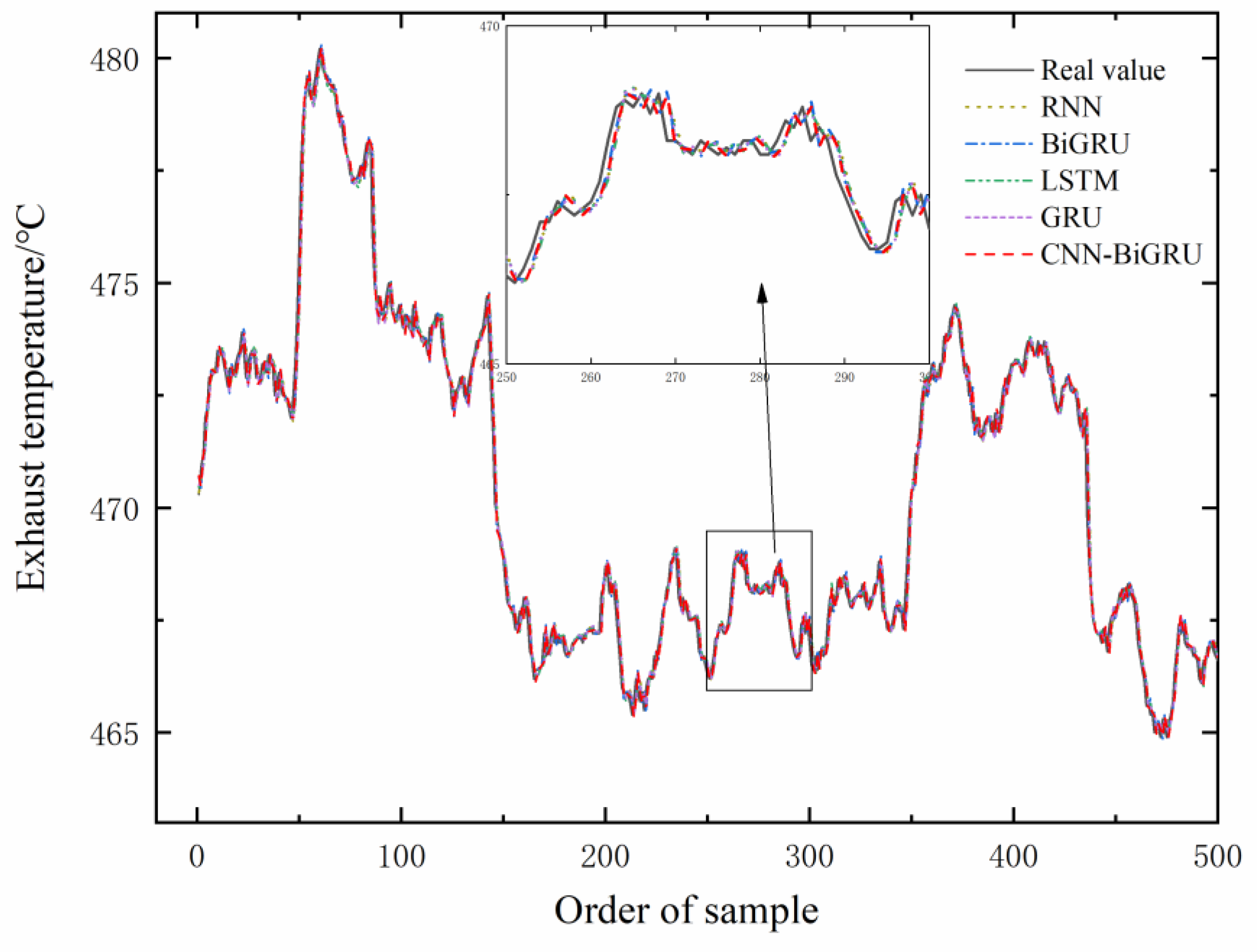
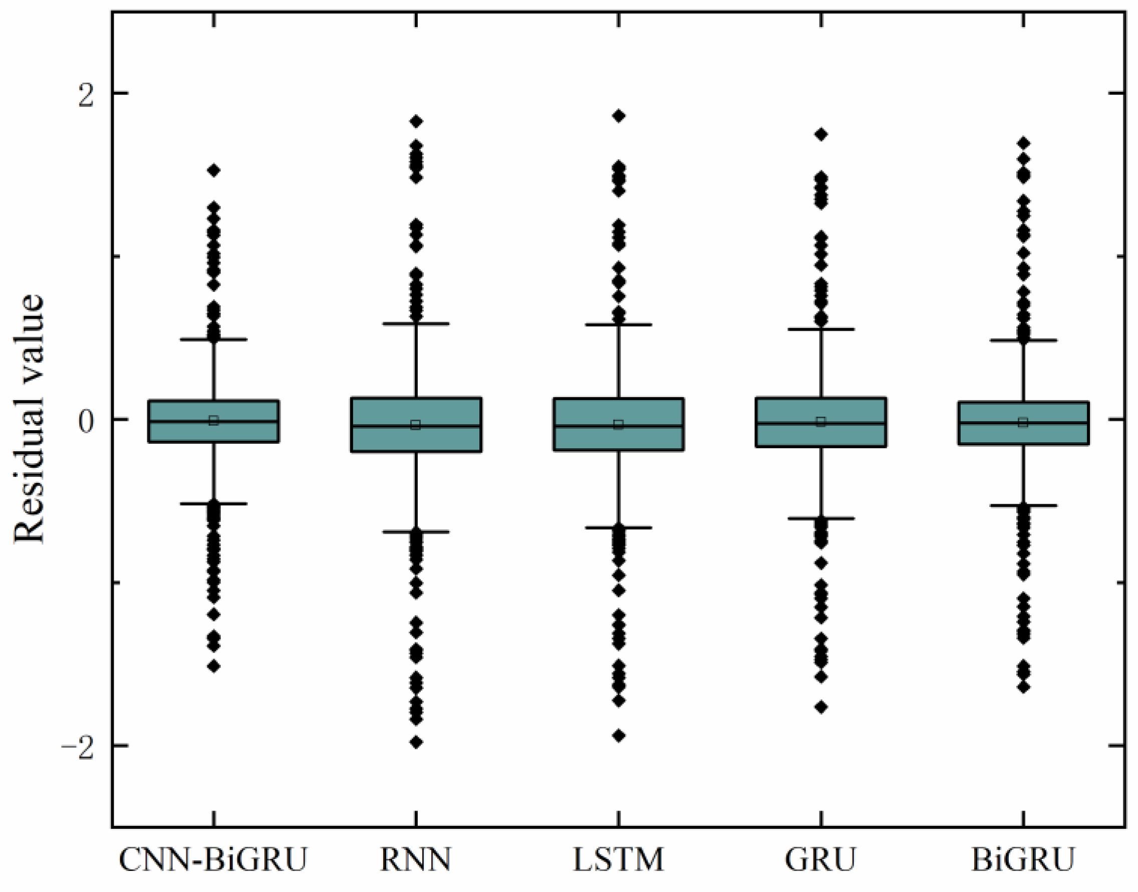
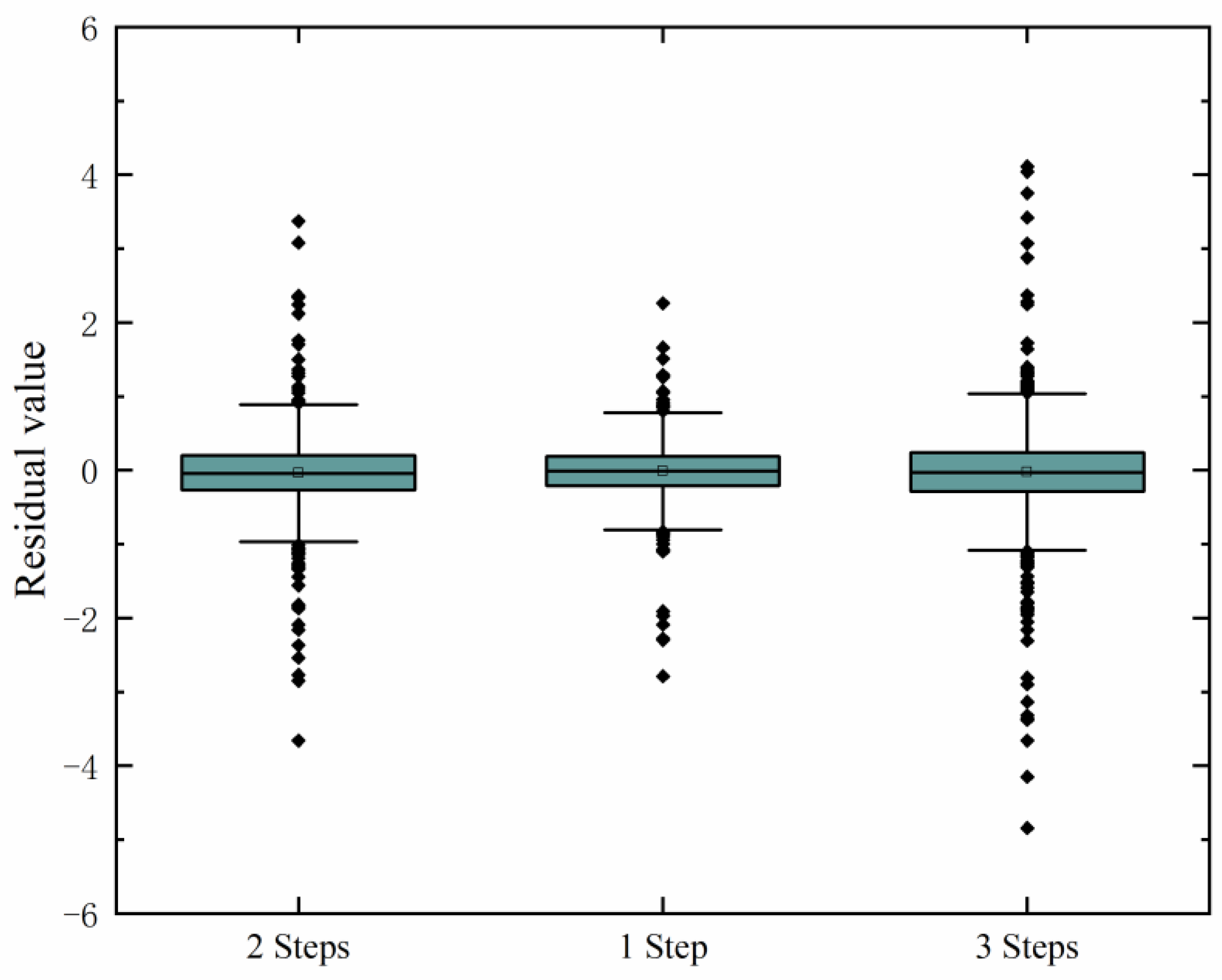
After the test is completed, the output evaluation indicators are shown in Table 6. The prediction result curve is shown in Figure 7. It can be concluded from Table 6 that, the evaluation index results of the prediction model proposed in this paper are respectively 0.2501, 0.1156, 0.0005336 for MAE, MSE and MAPE. Compared with other prediction models of the same type, the evaluation indicators of CNN-BiGRU are the smallest, indicating that its prediction accuracy is higher than that of other models. Further, combined with the boxplot of the residual values shown in Figure 8, it can be seen that the mean value of the prediction errors of all the prediction models in the experiment is close to 0. Still, the deviation of the prediction error of the CNN-BiGRU model proposed in this paper is significantly smaller, which shows that the CNN-BiGRU model has higher prediction accuracy and has an advantage in time series data prediction.

4. Fault Early Warning Research

4.1. The Number of Forecast Steps Is Determined

The number of prediction steps refers to the number of future state points predicted by the prediction model in advance, which reflects the ability of the prediction model to predict the length of time. In this article, the prediction steps are determined by the control variable method. We keep other parameters of the model unchanged, gradually increase the number of prediction steps, and observe the output results of the model. The prediction curve is shown in Figure 9, and the evaluation index results are shown in

Table 7. Evaluation metrics for different prediction steps.

Prediction Steps	MAE	MSE	MAPE
1 Step	0.2501	0.1156	0.0005336
2 Steps	0.3168	0.2011	0.0006758
3 Steps	0.3697	0.3038	0.0007884

. It can be seen from the results in Table 7 that, with the increase in the number of prediction steps, the evaluation indicators of the prediction results increase significantly. The residual boxplot combined with different prediction steps is shown in Figure 10. It can be seen that although the mean values of the errors of different prediction steps are close to 0, with the increase in step size, the degree of error deviation continues to increase. When the step size is selected as 1, the prediction result is better. Therefore, through the experimental demonstration in this part, the prediction step size of the model output is chosen as 1.

4.2. Early Warning Value Setting

The setting of the alarm threshold is the most important part of the research on fault early warning. For marine power generation diesel engines that have been in stable working conditions for a long time, if the alarm threshold is set too high, it is difficult to achieve fault early warning at the early stage of prediction, and it is impossible to send an alarm to managers in advance. If the alarm threshold is too small, it is easy to cause a false alarm when the load changes slightly.

In this paper, the historical data of the normal operation of the marine power generation diesel engine is used and input into the proposed CNN-BiGRU prediction model after data processing. When the diesel engine operates normally, the exhaust temperature of the diesel engine is relatively stable, so the prediction error value of the model is relatively small. When a potential failure occurs in a diesel engine, the degree of failure will increase as operating time increases, and the exhaust temperature will deviate from the normal range, which will lead to an increase in the prediction error of the prediction model. Therefore, the upper and lower limits of the residual value are set by using the residual value distribution curve and the statistical process control method [44]. Then, the sliding window algorithm is used to calculate the standard deviation corresponding to each window of the residual distribution, and then we can set the upper limit of the standard deviation. The alarm threshold for diesel engine exhaust temperature is set by the two thresholds calculated. The formula for calculating the standard deviation of the sliding window is as follows.

$$S=\sqrt{\frac{1}{N-1}{\displaystyle \sum _{i=1}^N{(e_i-\overline{X})}^2}}$$

(10)

In the formula, N represents the size of the sliding window; e_i represents the residual value at i in this window; and $\overline{X}$ represents the mean value of all residual values in the window.

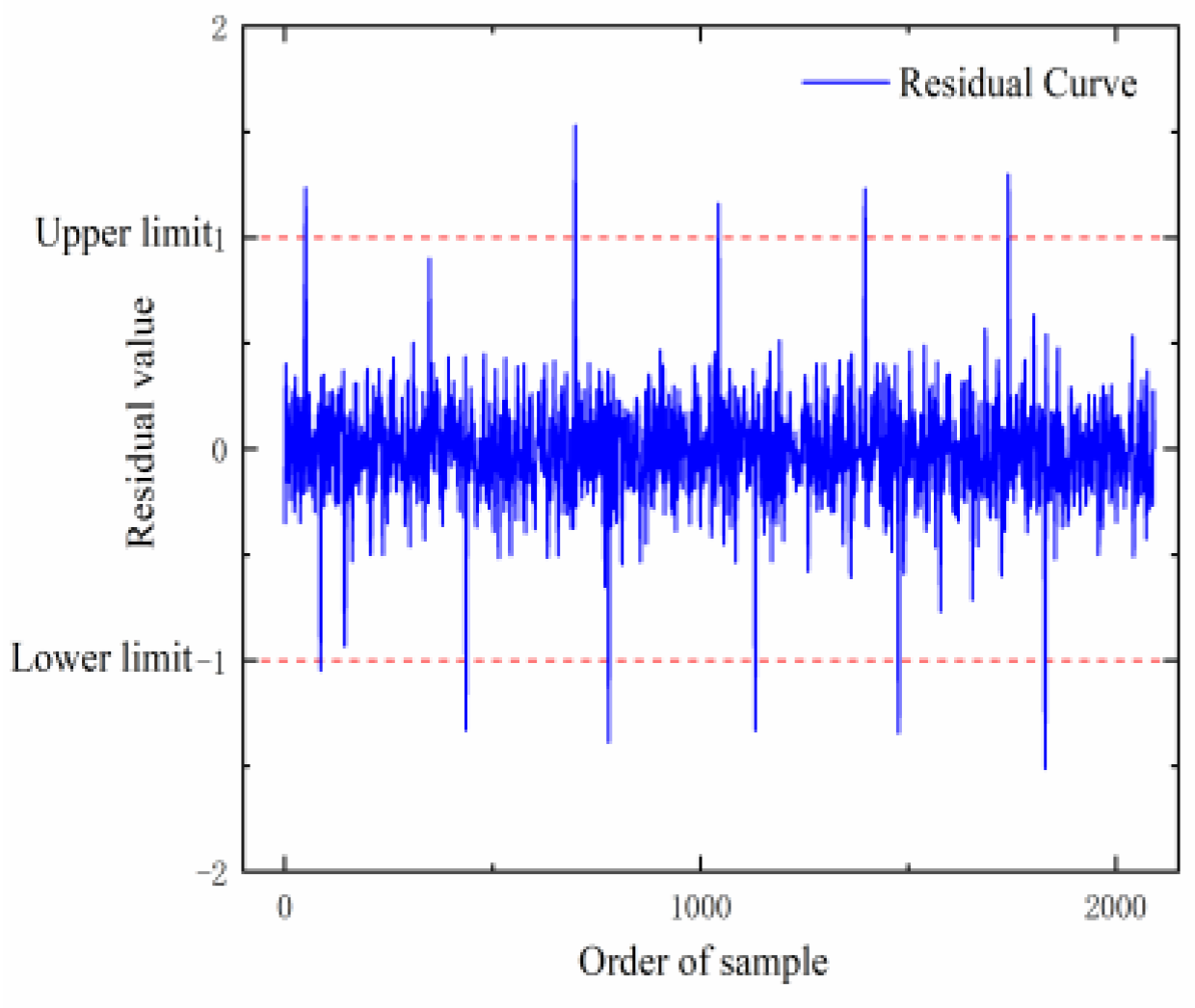
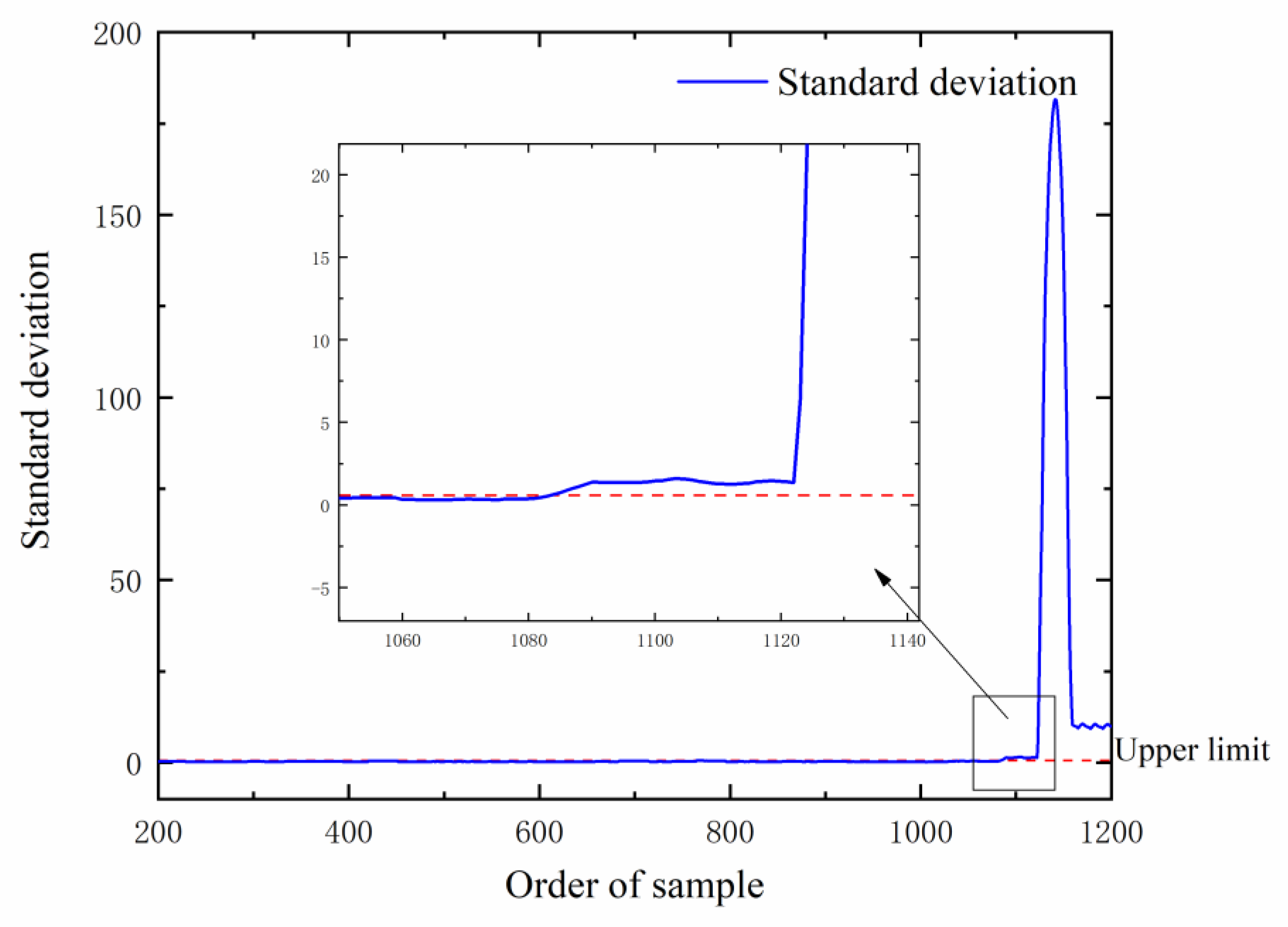
The residual distribution curve is drawn according to the prediction results of normal operation data, as shown in Figure 11. It can be seen from Figure 11 that the range of residual values between the predicted results and the true values is basically between −1 and 1. Combined with the number of residuals (S) in each area in

Table 8. Statistical Table of Residual Values under Normal Working Conditions.

Interval	Quantity	Cumulative Percentage	Interval	Quantity	Cumulative Percentage
−3 ≤ R < −2.5	1	0.0478	−0.5 ≤ R < 0	960	51.86424
−2.5 ≤ R < −2	3	0.1912	0 ≤ R < 0.5	904	95.07648
−2 ≤ R < −1.5	2	0.28681	0.5 ≤ R < 1	94	99.56979
−1.5 ≤ R < −1	4	0.47801	1 ≤ R < 1.5	6	99.8566
−1 ≤ R < −0.5	115	5.97514	1.5 ≤ R < 2	2	99.9522

, it can be obtained that the cumulative percentage of the number of residuals in the range of −1~1 can reach more than 99%, indicating that the deviation between the predicted value and the actual value under normal and stable conditions is 99% likely to fall between −1~1. Therefore, the upper alarm limit of the residual value is set to 1, and the lower alarm line is set to −1, as shown in Figure 12. A large number of the residual values in the figure are within the set range, but there are still very few residual values that deviate greatly beyond the set threshold range, which may lead to false alarms. The standard deviation is the most commonly used quantitative form to reflect the dispersion degree of a group of data. Therefore, in addition to analyzing the residual distribution, the sliding window is used to analyze and process the standard deviation of the residual value. Based on manual experience, set the sliding window size to 30 and calculate the standard deviation of the residual value. The changing trend of the residual standard deviation after processing is shown in Figure 13. It can be seen from Figure 13 that the maximum standard deviation of the residual error is 0.604 when the diesel engine is operating under stable conditions. It can be seen that the residual early warning value of the marine diesel generator is ±1, and the early warning value of the residual standard deviation is 0.604. Only when two early warning values exceed the limit at the same time, the alarm will be triggered.

4.3. Experiment Analysis

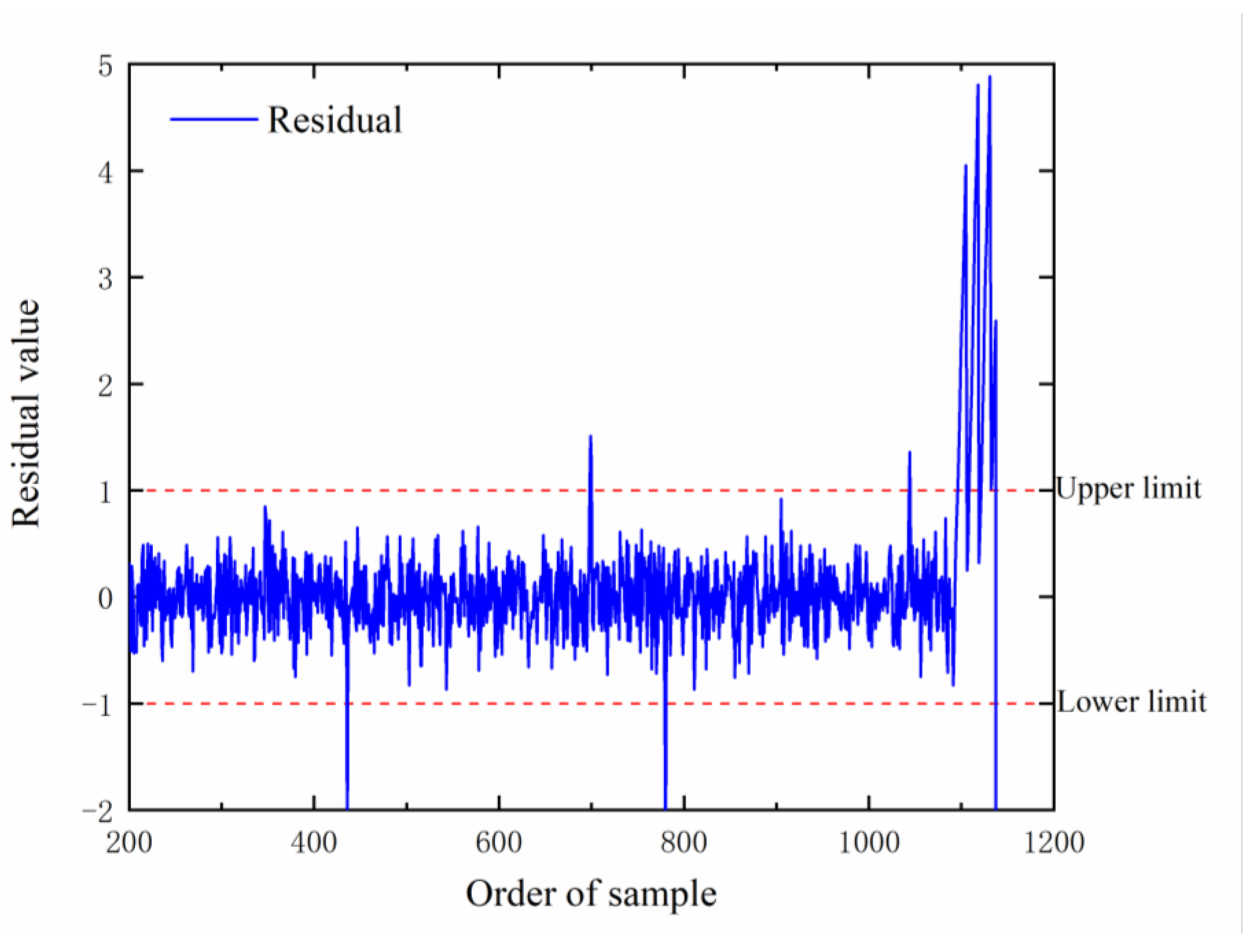
Considering that the data set collected in this paper does not contain fault data, in order to verify the effectiveness of the proposed method, the data set is artificially adjusted linearly to simulate fault conditions to generate an artificial data set. It can be seen from the above part that the alarm threshold for fault early warning is that the residual value is greater than 1 or less than −1, and the standard deviation calculated by using the sliding window is more than 0.604. When the two situations occur at the same time, a potential failure alarm can be issued to prompt the management personnel to pay attention to the operation status of the diesel engine and take corresponding measures. Exhaust gas temperature is a slow-changing thermal parameter. When the diesel engine has early failure characteristics, it will change slowly. As the degree of failure increases, the change will gradually increase. After the temperature rises or falls to a certain level, it will stop. When the exhaust gas temperature rises abnormally, the predicted graph of the exhaust temperature is shown in Figure 14. From Figure 14, it can be seen that the predicted value is very close to the actual value before the abnormal temperature increase. However, the deviation between the predicted and actual values gradually increases after the abnormal rise in exhaust gas temperature is set at 1096. Combined with the residual curve graph shown in Figure 15, the residual values are basically within the set upper and lower limits until sample point 1096. Although there are a few sample points that exceed the threshold, according to the standard deviation curve graph shown in Figure 16, it can be seen that the standard deviation of the residual values calculated using the sliding window does not exceed the set threshold until sample point 1082, so no fault warning occurs until sample point 1096. After setting the abnormal temperature increase at sample point 1096, the residual value rapidly exceeds the set threshold, and the standard deviation value already exceeds the set threshold at 1082. This indicates a potential failure of the diesel engine. Therefore, a fault warning will be achieved at 1096. It can be seen that when the diesel engine has a hidden fault and the exhaust temperature changes abnormally, the early warning method proposed in this paper can effectively detect the abnormal state of the diesel engine, send an alert to the manager in time, and also eliminate the possibility of an alarm occurring in the normal state.

5. Conclusions

This paper studies the problem of early warning of marine diesel engine faults and proposes a fault early warning method for marine diesel engines based on CNN-BiGRU. Conclusion as below:

Using the Pearson correlation coefficient to select the operating parameters that are highly correlated with the exhaust temperature as the input of the prediction model can effectively reduce the model input dimension, simplify the model structure, reduce the model calculation time, and reduce the model training load.

Aiming at the prediction of the exhaust temperature of diesel engine for marine power generation, this paper proposes a prediction method combining CNN and BiGRU, which extracts the features of multi-dimensional input variables through CNN and then uses the advantages of BiGRU in predicting time series data to predict the exhaust temperature of a diesel engine. The prediction results show that there is less deviation between the predicted value and the actual value, and the prediction accuracy is higher. In order to verify the effectiveness of the model proposed in this paper, it is compared with RNN, LSTM, GRU, and BiGRU. Firstly, the convergence speed of the model proposed in this paper is significantly faster than that of other models in the training process. Then, compare the time required by different models to predict a step. The results show that the time required by the proposed model to predict a step is only 0.066 s. Compared with the other four models, the time is reduced by 0.424 s, 0.364 s, 0.342 s, and 0.264 s, respectively. It reflects the advantages of the model in predicting time consumption. Finally, the prediction results of CNN-BiGRU are compared with those of the above four models. In contrast, the MSE decreased by 0.0307, 0.0233, 0.013, and 0.0078, respectively; the MAE decreased by 0.0225, 0.0174, 0.0092, and 0.0102, respectively; and the MAPE decreased by 0.0000477, 0.000037, 0.0000191, and 0.0000236, respectively. The experimental results show that the prediction accuracy of the method proposed in this paper is higher, which further demonstrates the advantages of the CNN–BiGRU combined model in time series data prediction.

Through the comparison of the forecast duration and the analysis of the forecast residual value, the forecast duration is determined, and the alarm threshold for the forecast residual value and standard deviation value is set. Through the experimental verification analysis, the method used can detect the abnormal state of the diesel engine in time and provide strong support for the state detection and health management of the marine diesel engine.

In summary, the fault early warning method of the marine diesel engine proposed in this paper not only provides a new reference for the health management of the marine diesel engine but also has a certain reference significance for the prediction of future states and abnormal detection of intelligent marine equipment. However, we have only performed condition prediction as well as fault warning for the marine diesel engine under steady-state operation. In addition, the model can only recognize the abnormal operation state of a diesel engine at the early stage of a fault but cannot realize fault diagnosis. In our future work, we will collect operating data under different states to identify the operating state of the diesel engine and also collect early fault data as much as possible to achieve fault localization and continue to improve the function of the model.

References

1. Liao, J.B.; Yuan, H.; Zhong, H.; Huang, Y. Research on Fault Early Warning Method of Diesel Generator Based on Infrared Image. In Proceedings of the 2nd International Conference on Optics and Image Processing (ICOIP), Xi’an, China, 7–9 April 2022. [Google Scholar]
2. Hvozdeva, I.; Myrhorod, V.; Budashko, V.; Shevchenko, V. Problems of Improving the Diagnostic Systems of Marine Diesel Generator Sets. In Proceedings of the 15th International Conference on Advanced Trends in Radioelectronics, Telecommunications and Computer Engineering (TCSET), Lviv, Ukraine, 25–29 February 2020. [Google Scholar]
3. Rudzki, K.; Gomulka, P.; Hoang, A. Optimization Model to Manage Ship Fuel Consumption and Navigation Time. Pol. Marit. Res. 2022, 29, 141–153. [Google Scholar] [CrossRef]
4. Ma, Q.; Chen, B.; Jia, B. Development of Monitoring and Fault Expert System for Marine Generator Diesel Based on Lab VIEW. In Proceedings of the Annual Conference of China-Institute-of-Communications, Guangzhou, China, 26 November 2009. [Google Scholar]
5. Feng, S.S.; Chen, Z.; Guan, Q.; Yue, J.; Xia, C. Grey Relational Analysis-Based Fault Prediction for Watercraft Equipment. Front. Phys. 2022, 10, 1–7. [Google Scholar] [CrossRef]
6. Gao, Z.; Jiang, Z.; Zhang, J. Identification of power output of diesel engine by analysis of the vibration signal. Meas. Control 2019, 52, 1371–1381. [Google Scholar] [CrossRef] [Green Version]
7. Che, C.C.; Wang, H.; Fu, Q.; Ni, X. Intelligent fault prediction of rolling bearing based on gate recurrent unit and hybrid autoencoder. Proc. Inst. Mech. Eng. Part C J. Mech. Eng. Sci. 2021, 235, 1106–1114. [Google Scholar] [CrossRef]
8. Kumar, A.; Srivastava, A.; Goel, N.; McMaster, J. EXHAUST GAS TEMPERATURE DATA PREDICTION BY AUTOREGRESSIVE MODELS. In Proceedings of the IEEE 28th Canadian Conference on Electrical and Computer Engineering (CCECE), Halifax, NS, Canada, 3–6 May 2015. [Google Scholar]
9. Zhang, Y.F.; Liu, P.; He, X.; Jiang, Y. A prediction method for exhaust gas temperature of marine diesel engine based on LSTM. In Proceedings of the 2nd IEEE International Conference on Civil Aviation Safety and Information Technology (ICCASIT), Wuhan, China, 14–16 October 2020. [Google Scholar]
10. Zhang, B.S.; Zhang, L.; Zhang, B.; Yang, B.; Zhao, Y. A Fault Prediction Model of Adaptive Fuzzy Neural Network for Optimal Membership Function. IEEE Access 2020, 8, 101061–101067. [Google Scholar] [CrossRef]
11. Caliwag, A.; Han, S.; Park, K.; Lim, W. Deep-Learning-Based Fault Occurrence Prediction of Public Trains in South Korea. Transp. Res. Rec. 2022, 2676, 710–718. [Google Scholar] [CrossRef]
12. Kusiak, A.; Li, W. The prediction and diagnosis of wind turbine faults. Renew. Energy 2011, 36, 16–23. [Google Scholar] [CrossRef]
13. Li, C.C.; Guo, C.; Xue, Y. Early Warning Model of Engine Fault of Liquefied Natural Gas Bus. In Proceedings of the 8th International Conference on Logistics, Informatics and Service Sciences (LISS), Toronto, ON, Canada, 3–6 August 2018. [Google Scholar]
14. Liu, G.J.; Gu, H.; Shen, X.; You, D. Bayesian Long Short-Term Memory Model for Fault Early Warning of Nuclear Power Turbine. IEEE Access 2020, 8, 50801–50813. [Google Scholar] [CrossRef]
15. Zhang, W.; Liu, J.; Gao, M.; Pan, C. A fault early warning method for auxiliary equipment based on multivariate state estimation technique and sliding window similarity. Comput. Ind. 2019, 107, 67–80. [Google Scholar] [CrossRef]
16. Liang, T.; Qian, S.; Meng, Z.; Xie, G. Early fault warning of wind turbine based on BRNN and large sliding window. J. Intell. Fuzzy Syst. 2020, 38, 3389–3401. [Google Scholar] [CrossRef]
17. Yuan, L.; Qiu, L.; Zhang, C. Research on Normal Behavior Models for Status Monitoring and Fault Early Warning of Pitch Motors. Appl. Sci. 2022, 12, 7747. [Google Scholar] [CrossRef]
18. Yan, X.; Liu, C. Wind Turbine Gearbox fault early warning based on NEST. In Proceedings of the 5th International Conference on Environment, Materials, Chemistry and Power Electronics (EMCPE), Zhengzhou, China, 11–12 April 2016. [Google Scholar]
19. Liu, Y.; Gan, H.; Cong, Y.; Hu, G. Research on fault prediction of marine diesel engine based on attention-LSTM. Inst. Mech. Eng. Part M J. Eng. Marit. Environ. 2022. [Google Scholar] [CrossRef]
20. Desbazeille, M.; Randall, R.; Guillet, F.; El Badaoui, M.; Hoisnard, C. Model-based diagnosis of large diesel engines based on angular speed variations of the crankshaft. Mech. Syst. Signal Process. 2010, 24, 1529–1541. [Google Scholar] [CrossRef]
21. Cheliotis, M.; Lazakis, I.; Theotokatos, G. Machine learning and data-driven fault detection for ship systems operations. Ocean. Eng. 2020, 216, 107968. [Google Scholar] [CrossRef]
22. Han, P.H.; Ellefsen, A.; Li, G.; Aelig, V.; Zhang, H. Fault Prognostics Using LSTM Networks: Application to Marine Diesel Engine. IEEE Sens. J. 2021, 21, 25986–25994. [Google Scholar] [CrossRef]
23. Theodoropoulos, P.; Spandonidis, C.; Giannopoulos, F.; Fassois, S. A Deep Learning-Based Fault Detection Model for Optimization of Shipping Operations and Enhancement of Maritime Safety. Sensors 2021, 21, 5658. [Google Scholar] [CrossRef] [PubMed]
24. Che, C.C.; Wang, H.; Fu, Q.; Ni, X. Combining multiple deep learning algorithms for prognostic and health management of aircraft. Aerosp. Sci. Technol. 2019, 94, 105423. [Google Scholar] [CrossRef]
25. Shuai, Y. Research on Fault Diagnosis Technology of Industrial Robot Operation Based on Deep Belief Network. Sci. Program. 2022, 2022, 1–12. [Google Scholar] [CrossRef]
26. Karatu, C.; Arslanoglu, Y. Development of condition-based maintenance strategy for fault diagnosis for ship engine systems. Ocean. Eng. 2022, 256, 111515. [Google Scholar] [CrossRef]
27. Lazakis, I.; Raptodimos, Y.; Varelas, T. Predicting ship machinery system condition through analytical reliability tools and artificial neural networks. Ocean Eng. 2018, 152, 404–415. [Google Scholar] [CrossRef]
28. Vos, K.; Peng, Z.; Jenkins, C.; Shahriar, M.; Borghesani, P.; Wang, W. Vibration-based anomaly detection using LSTM/SVM approaches. Mech. Syst. Signal Process. 2022, 169, 108752. [Google Scholar] [CrossRef]
29. Kichan, S.; Lee, K.; Byun, S. A study on fault diagnosis of marine engine using a neural network with dimension-reduced vibration signals. J. Acoust. Soc. Korea 2022, 41, 492–499. [Google Scholar]
30. Velasco-Gallego, C.; Lazakis, I. RADIS: A real-time anomaly detection intelligent system for fault diagnosis of marine machinery. Expert Syst. Appl. 2022, 204, 117634. [Google Scholar] [CrossRef]
31. Chernyi, S.; Emelianov, V.; Zinchenko, E.; Zinchenko, A.; Tsvetkova, O.; Mishin, A. Application of Artificial Intelligence Technologies for Diagnostics of Production Structures. J. Mar. Sci. Eng. 2022, 10, 259. [Google Scholar] [CrossRef]
32. Theodoropoulos, P.; Spandonidis, C.; Fassois, S. Use of Convolutional Neural Networks for vessel performance optimization and safety enhancement. Ocean. Eng. 2022, 248, 110771. [Google Scholar] [CrossRef]
33. Dong, H.; Lu, J.; Han, Y. Multi-Stream Convolutional Neural Networks for Rotating Machinery Fault Diagnosis under Noise and Trend Items. Sensors 2022, 22, 2720. [Google Scholar] [CrossRef]
34. Dashti, R.; Daisy, M.; Mirshekali, H.; Shaker, H.; Aliabadi, M. A survey of fault prediction and location methods in electrical energy distribution networks. Measurement 2021, 184, 109947. [Google Scholar] [CrossRef]
35. Wei, Z.P.; Davison, A. A convolutional neural network based model to predict nearshore waves and. Coast. Eng. 2022, 171, 104044. [Google Scholar] [CrossRef]
36. Lee, L.; Xie, L.; Zhang, D.; Yu, B.; Ge, Y.; Lin, F. Condition Assessment of Power Transformers Using a Synthetic Analysis Method Based on Association Rule and Variable Weight Coefficients. IEEE Trans. Dielectr. Electr. Insul. 2013, 20, 2052–2060. [Google Scholar]
37. Chen, Z.S.; Zhang, L.; Hua, J.; Kim, B.; Li, K.; Xue, X. A framework of data-driven wind pressure predictions on bluff bodies using a hybrid deep learning approach. Meas. Control 2022. [Google Scholar] [CrossRef]
38. Guo, L.; Qin, Z.; Ge, P.; Gao, T. Adaptive Lane-Departure Prediction Method with Support Vector Machine and Gated Recurrent Unit Models. J. Transp. Eng. Part A Syst. 2022, 148, 04022103. [Google Scholar] [CrossRef]
39. Yu, J.X.; Zhang, X.; Xu, L.; Dong, J.; Zhangzhong, L. A hybrid CNN-GRU model for predicting soil moisture in maize root zone. Agric. Water Manag. 2021, 245, 106649. [Google Scholar] [CrossRef]
40. Lu, Y.W.; Hsu, C.; Huang, K. An Autoencoder Gated Recurrent Unit for Remaining Useful Life Prediction. Processes 2020, 8, 1155. [Google Scholar] [CrossRef]
41. Zhang, B.; Jia, M.; Xu, J.; Zhao, W.; Deng, L. Network Security Situation Prediction Model Based on EMD and ELPSO Optimized BiGRU Neural Network. Comput. Intell. Neurosci. 2022, 2022, 1–17. [Google Scholar] [CrossRef] [PubMed]
42. Elsayed, N.; Maida, A.; Bayoumi, M. Gated Recurrent Neural Networks Empirical Utilization for Time Series Classification. In Proceedings of the IEEE Int Congr on Cybermat/12th IEEE Int Conf on Cyber, Phys and Social Comp (CPSCom)/15th IEEE Int Conf on Green Computing and Communications (GreenCom)/12th IEEE Int Conf on Internet of Things (iThings)/5th IEEE Int Conf on Smart Data, Atlanta, GA, USA, 14–17 July 2019. [Google Scholar]
43. Teng, W.; Cheng, L.; Zhao, K. Application Of Kernel Principal Component And Pearson Correlation Coefficient In Prediction Of Mine Pressure Failure. In Proceedings of the Chinese Automation Congress (CAC), Jinan, China, 30 Novenber–2 December 2017. [Google Scholar]
44. Wang, F.F.; Xiao, X.; Zhao, H. Wind turbine gearbox failure prediction based on time series analysis and statistical process control. In Proceedings of the International Conference on Energy, Environment and Sustainable Development (ICEESD 2011), 2011, Shanghai Univ Elect Power, Shanghai, China, 11 October 2011. [Google Scholar]
Figure 1. The convolutional neural network structure diagram.
Jmse 11 00056 g001
Figure 2. The GRU structure diagram.
Jmse 11 00056 g002
Figure 3. The BiGRU structure diagram.
Jmse 11 00056 g003
Figure 4. CNN-BiGRU prediction model structure diagram.
Jmse 11 00056 g004
Figure 5. CNN-BiGRU prediction results.
Jmse 11 00056 g005
Figure 6. Training loss curves of different models.
Jmse 11 00056 g006
Figure 7. Comparison results from different models.
Jmse 11 00056 g007
Figure 8. Prediction result residual value box plot.
Jmse 11 00056 g008
Figure 9. Comparison of the results of different prediction steps.
Jmse 11 00056 g009
Figure 10. Boxplot of residual values at different forecast steps.
Jmse 11 00056 g010
Figure 11. Distribution map of residual value under normal working conditions.
Jmse 11 00056 g011
Figure 12. Normal operating condition residual value curve.
Jmse 11 00056 g012
Figure 13. Normal working condition standard deviation curve.
Jmse 11 00056 g013
Figure 14. Abnormal condition exhaust temperature prediction.
Jmse 11 00056 g014
Figure 15. Residual curve plot of abnormal state.
Jmse 11 00056 g015
Figure 16. Standard deviation curve of abnormal state.
Jmse 11 00056 g016