A Multi-Objective Mission Planning Method for AUV Target Search

Abstract

How an autonomous underwater vehicle (AUV) performs fully automated task allocation and achieves satisfactory mission planning effects during the search for potential threats deployed in an underwater space is the focus of the paper. First, the task assignment problem is defined as a traveling salesman problem (TSP) with specific and distinct starting and ending points. Two competitive and non-commensurable optimization goals, the total sailing distance and the turning angle generated by an AUV to completely traverse threat points in the planned order, are taken into account. The maneuverability limitations of an AUV, namely, minimum radius of a turn and speed, are also introduced as constraints. Then, an improved ant colony optimization (ACO) algorithm based on fuzzy logic and a dynamic pheromone volatilization rule is developed to solve the TSP. With the help of the fuzzy set, the ants that have moved along better paths are screened and the pheromone update is performed only on preferred paths so as to enhance pathfinding guidance in the early stage of the ACO algorithm. By using the dynamic pheromone volatilization rule, more volatile pheromones on preferred paths are produced as the number of iterations of the ACO algorithm increases, thus providing an effective way for the algorithm to escape from a local minimum in the later stage. Finally, comparative simulations are presented to illustrate the effectiveness and advantages of the proposed algorithm and the influence of critical parameters is also analyzed and demonstrated.

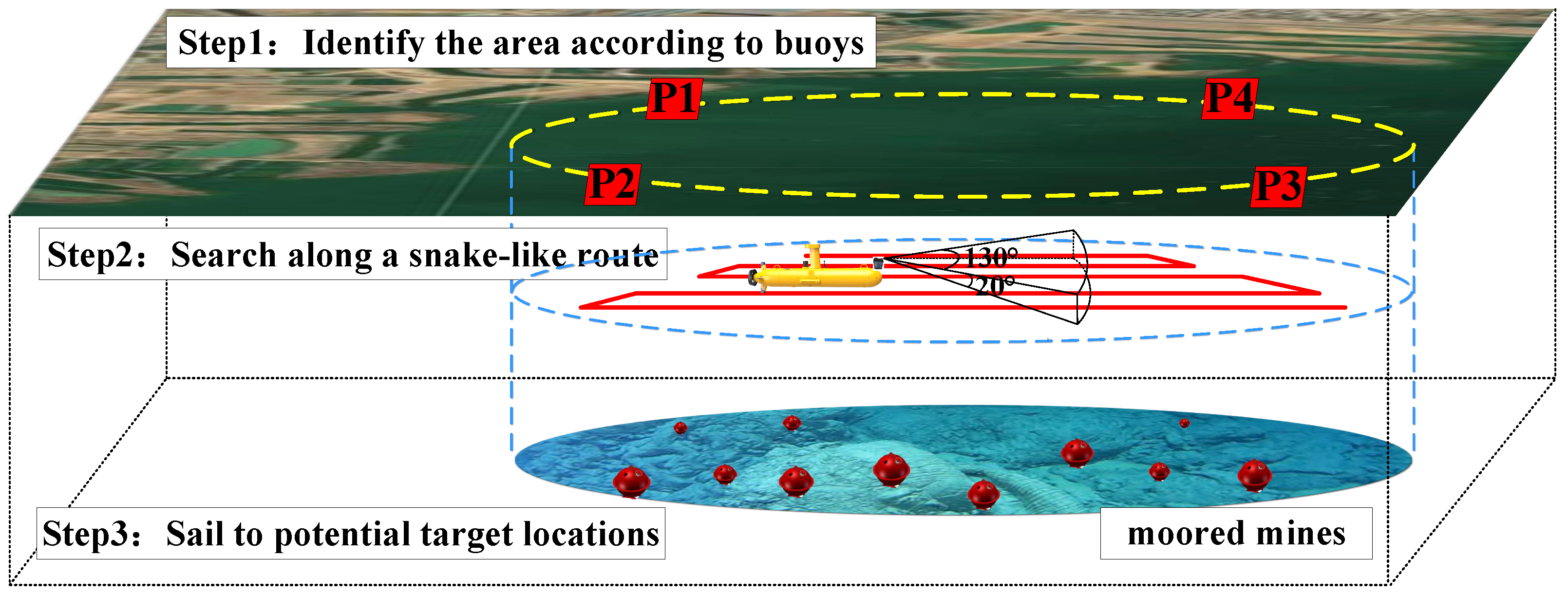
1. Introduction

Due to an increasing number of maritime accidents, underwater object detection applications such as search [1,2,3], rescue and track [4,5,6] missions have received extensive attention in both the civil and military fields. How to use existing equipment to quickly and accurately detect and identify high-value targets in underwater environments has become an urgent problem. Nowadays, intelligent equipment is widely researched [7,8]. AUVs are recognized as appropriate platforms to complete wide-area search missions [9,10]. When operating underwater, the AUV uses a forward-looking sonar mounted on the bow to detect targets of concern along a snake-like route that covers a designated area. If a series of suspected targets are detected, then the AUV will sail to each possible target location and conduct another close inspection, see Figure 1 for illustration. In this process, the autonomous task allocation capability of an AUV is particularly significant because it is necessary to determine the best order of approaching all targets, which can be described as a TSP [11].

For the TSP, methods for solving the problem mainly include exact algorithms, approximate algorithms and intelligent optimization algorithms. An exact algorithm involves integer linear programming algorithms, dynamic programming algorithms and graph algorithms [12], which can find a solution with an optimal value more efficiently, while the combinatorial explosion of the search space and long searching time pose challenges. The approximate algorithms contain insertion algorithms and nearest neighbor algorithms [13]. Although the method can quickly obtain a feasible solution, the result is not satisfactory as an optimization problem. Intelligent optimization algorithms include ACO algorithms [14,15,16], genetic algorithms [17,18,19], particle swarm optimization algorithms [20,21,22] and so on. Since intelligent optimization algorithms can find a satisfactory solution or an approximate optimal solution in a relatively short time, they have broad application prospects in the TSP and other optimization problems [23]. Compared with genetic algorithms (which possess a weak local search ability and suffer from the phenomenon of premature convergence [24]) and particle swarm optimization algorithms (which reveal a diminished search ability and a decreasing convergence rate in the later stage [25]), the ACO algorithms have remarkable benefits consisting of a dispersed calculative mechanism, strong robustness and greedy heuristic search functions [26]. Regarding ACO algorithms, many improvement methodologies and techniques have been put forward by scholars in related fields at home and abroad. The work in [27] introduced a negative feedback mechanism into the ACO algorithm by summarizing wrong experiences from historical information to help ants explore more unknown areas. The improved ACO algorithm promoted diverse solutions and prevented solutions from falling into local optima at the expense of convergence speed. The work in [28] integrated dynamic elitist ants, repeated annealing, pheromone variation and two-optimization local search strategies with the ACO algorithm, which enhanced the efficiency and accuracy of the algorithm; however, further acceleration of convergence speed was still needed. In [29], a cooperative model, a mean filtering approach and an entropy-based learning strategy were combined with the ACO algorithm to promote the diversity of solutions and prevent solutions from falling into local optima, but the disadvantage of slow convergence of the algorithm should be addressed. In [30], a dynamic evaporation strategy was integrated into the ACO algorithm to improve uncertain convergence time and random decisions, but the trend of becoming stuck on local optima in the later stages of the algorithm should be improved. A variable-step ACO algorithm was proposed in [31] to optimize the distribution of pheromones, reduce the influence of local pheromone concentrations and reduce the number of convergence iterations, but the ability to prevent falling into local optima is still needed. The work [32] delivered a pheromone updating mechanism, where speeding up the convergence of the algorithm relied on strengthening the updating of pheromones and refining the positive feedback of the optimal path. For the modified algorithm, an unsolved problem was that it was easy to become stuck on local optima in the later stage. Through the above-mentioned observations, we can see that the field of research in ACO algorithms for the TSP still bristles with difficulties, especially in terms of increasing ACO algorithm’s rate of convergence, as well as preventing its entrapment in local optimum. This provides motivation for the conception and development of the paper.

The paper concentrates on realizing an ACO algorithm based on fuzzy logic and a dynamic pheromone volatilization rule so as to generate a high-quality solution for the online task assignment problem in AUVs that is modeled as a multi-objective TSP. The main contributions of the paper are as follows:

(1)

Compared with the existing results in [27,28,29], the fuzzy logic theory is introduced, and the membership function involved is designed to evaluate the superiority and importance of the paths searched by ants. With the help of the membership degree, the differences in pheromone concentration between better and worse paths are amplified. The magnification of differences can better cultivate ants’ strong interest of selecting better paths and offer proper guidance on the choice of search direction during early stages of iterative optimization process.

(2)

Different from results in [30,31,32], our proposed ACO algorithm adds the concept of a dynamic pheromone volatilization rate. As iterations continue, driven by a dynamic update rule, the volatilization rate gradually increases so as to counteract the influence of positive feedback from the original ACO algorithm during later stages of the iterative optimization process. As a result, the global search ability of the algorithm is improved, and the problem of the algorithm falling into the local optimal solution is naturally avoided.

The rest of the paper is organized as follows. In Section 2, description of the task assignment problem for underwater target search is presented. Section 3 introduces the basic idea of the ACO algorithm. Section 4 describes the proposed routing protocol for an AUV with the support of an ACO algorithm, fuzzy logic and a dynamic pheromone volatilization rule. Simulation results are given in Section 5 that demonstrate the developed theory and technique. Finally, Section 6 concludes the paper and discusses the scope for future work.

2. Normalization of Multiple Objectives

In this paper, a multi-objective TSP with different starting and ending points is applied to represent the process of task allocation in an AUV’s target search mission. The maneuvering performance of a vehicle and optimization objectives related to the sailing distance and turning angle are considered when planning a path through all suspected target locations. Since there exists incommensurability between two optimization objectives, that is, the shortest total sailing distance and the smallest total turning angle, a single optimization objective is quantified as follows:

$$T_i=\frac{L_i}{v_1}+\frac{A_i\pi r}{180v_2},$$

(1)

$$T=\sum _{i=1}^{n-2}{T}_i+\frac{L_{n-1}}{v_1},$$

(2)

where $i=1,2,\cdots ,n-2$; n is the number of suspicious targets; and $v_1$ and $v_2$ are linear speeds (measured in knots) at straight segments and curves, respectively. As shown in Figure 2, r is the turning radius and $L_i$ and $A_i$ are the length and angle of rotation (measured in degrees) of the i-th path segment, respectively. T is the total operation time.

3. Basics of an ACO Metaheuristic

The ACO algorithm is a probabilistic technique for seeking the optimal path from source to destination, which employs artificial ants and adopts their self-selection and pheromone-based interaction to determine the best order of visiting all target locations. Initially, the algorithm starts with all ants selecting random paths in search of the desired targets around their source, by which multiple routes are opened up from source to destination. Then, a solution is constructed if an ant has inspected all the suspected targets between source and destination. Based on the quality of solutions, ants deposit a trail of pheromones on their return paths to the source. When all ants complete their tour, the pheromone on route segments is updated and the current iteration is finished. The original ant colony dies, and a new one performs a new round of search. In subsequent steps, the pheromone trails previously deposited on the path provide orientation cues for the following ants to choose their paths from source to destination in a probabilistic way. The probability of a particular path being selected is higher if it tracks a direction with a richer pheromone concentration. All aforementioned procedures are applied repeatedly until a termination criterion is satisfied. The vehicle is provided with the order in which possible points of interest locations are to be searched, and when the vehicle passes over all points for acoustic detection, a desired trajectory is generated.

Note that the ACO algorithm has characteristics of strong robustness, information positive feedback and parallel computing [33,34,35] and promotes applications in the field of task planning [36,37,38]. Due to the characteristic of positive feedback, the ants leave more pheromones on better paths and in turn more pheromones attract more ants. Positive information feedback provides aid to the whole system to evolve rapidly in the direction of the optimal solution. However, if the solution obtained by an ACO algorithm is suboptimal instead of optimal, it will make the algorithm become trapped into the local optimum, and it will face difficulties in jumping out of the local minimum. To cope with this problem, we improve the ACO algorithm by adding fuzzy logic and a dynamic pheromone volatilization rule.

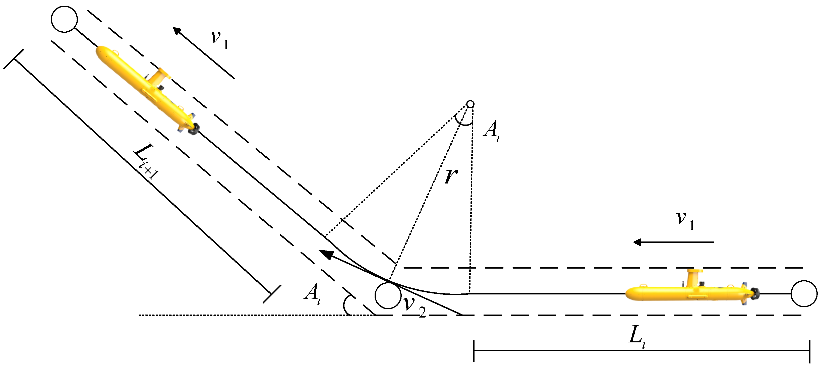
4. Method and Materials

4.1. Adjust Pheromone Release by Using Fuzzy Sets

In the traditional ACO algorithm, all ants release pheromones during each iteration. However, a notable difference in the paper is the integration of fuzzy logic into a traditional ACO algorithm to assist in picking better paths. The modified algorithm stipulates that only ants passing through the preferred paths have the ability to lay down pheromones at each iteration, with the purpose of providing guidance and support for the ant colony to find the optimal navigation path as soon as possible in the early stage of the algorithm.

In what follows, we first introduce concepts of a fuzzy set and degree of membership. Define a universe of discourse U and a fuzzy subset A in U; then, there is a membership degree $\mu \left(x\right)\in [0,1]$ for $\forall x\in U$ to indicate the certainty (or uncertainty) that element x belongs to A. To be specific, the closer the value of $\mu \left(x\right)$ is to 1, the more x certainly belongs to A, and the closer $\mu \left(x\right)$ is to 0, the lower the degree of x belonging to A is. In the paper, the universe of discourse U is denoted by $U=[minT,maxT]$, where $minT$ is the execution time corresponding to the fastest route in an iteration and $maxT$ is the time it takes for the ants to go through the longest path during an iteration. We let fuzzy subset A be filled with a collection of the total operation time related to “better paths”. The degree of membership of $T\left(k\right)$ in A is defined as follows:

$$\mu \left(k\right)=\mathrm{zmf}\left(T\right(k),minT,maxT),$$

(3)

where a Z-shaped membership function is applied

$$\mathrm{zmf}(T\left(k\right),minT,maxT)=\left\{\begin{array}{c}1,T\left(k\right)\le minT;\hfill \\ 1-2{\left(\frac{T\left(k\right)-minT}{maxT-minT}\right)}^2,minT\le T\left(k\right)\le \frac{minT+maxT}{2};\hfill \\ 2{\left(\frac{T\left(k\right)-maxT}{maxT-minT}\right)}^2,\frac{minT+maxT}{2}\le T\left(k\right)\le maxT;\hfill \\ 0,T\left(k\right)\ge maxT.\hfill \end{array}\right.$$

(4)

$T\left(k\right)$ denotes the travel time required for the k-th ant to traverse all waypoints in the current path in a single-iteration procedure.

After obtaining the membership degree of the path searched by each ant, we give a constant $\lambda \in [0,1]$ to evaluate the value of expression $\mu \left(k\right)$. It is stipulated that if membership degree $\mu \left(k\right)$ is greater than $\lambda$, then the corresponding k-th path is identified as a better path. The k-th ant will choose to pass through the better path and update pheromone concentration on each segment of the better path according to Equation (5). More specifically, the pheromone concentration on segments of the better path will be enhanced by the former equation in Formula (5), and meanwhile, the pheromone on segments of the path that ant k has not traveled will be suppressed by the following equation in Formula (5):

$${\tau }_{ijz}^t(t+1)=\left\{\begin{array}{c}(1-\rho ){\tau }_{ijz}^t\left(t\right)+\frac{KQ}{T\left(k\right)},\mathrm{if}\mathrm{ant}k\mathrm{passes}\mathrm{path}(i,j,z);\hfill \\ {\tau }_{ijz}^t\left(t\right)-\frac{Q\mu \left(k\right)}{T\left(k\right)},\mathrm{otherwise},\hfill \end{array}\right.$$

(5)

where $i,j,z$ are three vertices of a broken line; ${\tau }_{ijz}^t\left(t\right)$ is the pheromone quantity on polyline path $(i,j),(j,z)$ formed by connecting three points $i,j,z$ at current time instant t; Q is the total amount of pheromones released by performing a complete search on the current path; K is the pheromone amplification coefficient; $\rho$ and $1-\rho$ are the proportions of pheromone volatilization and pheromone residues with $\rho \in [0,1]$, respectively.

Different from the traditional ACO algorithm, the pheromone updating rule of the improved ACO algorithm adds two parts: a path importance factor and a penalty factor. In Equation (5), in the case of the k-th ant passing through path $(i,j,z)$, $(1-\rho ){\tau }_{ijz}^t\left(t\right)$ indicates the remnants of pheromone per unit time that remains on polyline path $(i,j),(j,z)$. $Q/\phantom{QT\left(k\right)}T\left(k\right)$ represents the average pheromone relative to a complete path. The function of parameter K is to give additional compensation to the pheromone increment so as to counteract the influence of natural volatilization on pheromone concentration. Since the effect of K can cover that of $\mu \left(k\right)$, the pheromone update item is designed as $KQ/\phantom{KQT\left(k\right)}T\left(k\right)$ instead of $KQ\mu \left(k\right)/\phantom{KQ\mu \left(k\right)T\left(k\right)}T\left(k\right)$. Another case of Equation (5) is set for path segments which the k-th ant has not traversed. In order to speed up the convergence of the modified algorithm, we introduce a penalty term $Q\mu \left(k\right)/\phantom{Q\mu \left(k\right)T\left(k\right)}T\left(k\right)$, which is set on the path that ants do not pass. The benefit of adopting a penalty strategy is that the dissimilarity between better and worse paths in terms of pheromone concentration is magnified, resulting in a better search guidance being developed in the early stage of the algorithm. The reason that $\mu \left(k\right)$ exists in the penalty term is to further distinguish the quality of the path and increase the difference. Specifically, the larger the $\mu \left(k\right)$, the better the path found by the k-th ant. In the design process, we want to enhance penalties for the path that ant k has not traveled, so $\mu \left(k\right)$ is applied. Moreover, compared with the original algorithm where the pheromone update takes into account the sum of new changes in pheromone with respect to all ants passing through the path segment, the proposed algorithm focuses on how changes in individual ants’ pheromones affect their own path choices.

4.2. Adjusting Pheromone Volatilization by Using a Dynamic Volatility Strategy

Observing Equation (5), it can be seen that pheromone concentration on a path is also affected by the pheromone volatilization rate $\rho$. In the original algorithm, $\rho$ is a constant, while in the modified algorithm, it changes dynamically according to the following rule:

$$\rho =\left\{\begin{array}{c}{\rho }_0+NC\frac{{\rho }_{max}-{\rho }_0}{N{C}_{max}},\mathrm{if}\mu \left(k\right)>\lambda ;\hfill \\ 0,\mathrm{otherwise},\hfill \end{array}\right.$$

(6)

where ${\rho }_0$ and ${\rho }_{max}$ are the initial value and the maximum value of pheromone volatilization rate, respectively. $NC$ is the current iteration’s number, and $N{C}_{max}$ is the maximum number of iterations in the loop.

The successive alteration of $\rho$ makes pheromone levels gradually decrease as iterations continue. As a result, the positive feedback effect of the algorithm is weakened in subsequent iterations. By appropriately reducing the pheromone on the previously selected better path, the gap between the pheromone and the pheromone on the untraveled path is narrowed, thereby expanding the search range and facilitating the global search capability. This is also the reason that we use ${\tau }_{ijz}^t\left(t\right)$ rather than $\left(1-\rho \right){\tau }_{ijz}^t\left(t\right)$ to design the penalty term in Equation (5). If $\left(1-\rho \right){\tau }_{ijz}^t\left(t\right)$ is employed, the effect of narrowing the gap would be greatly diminished.

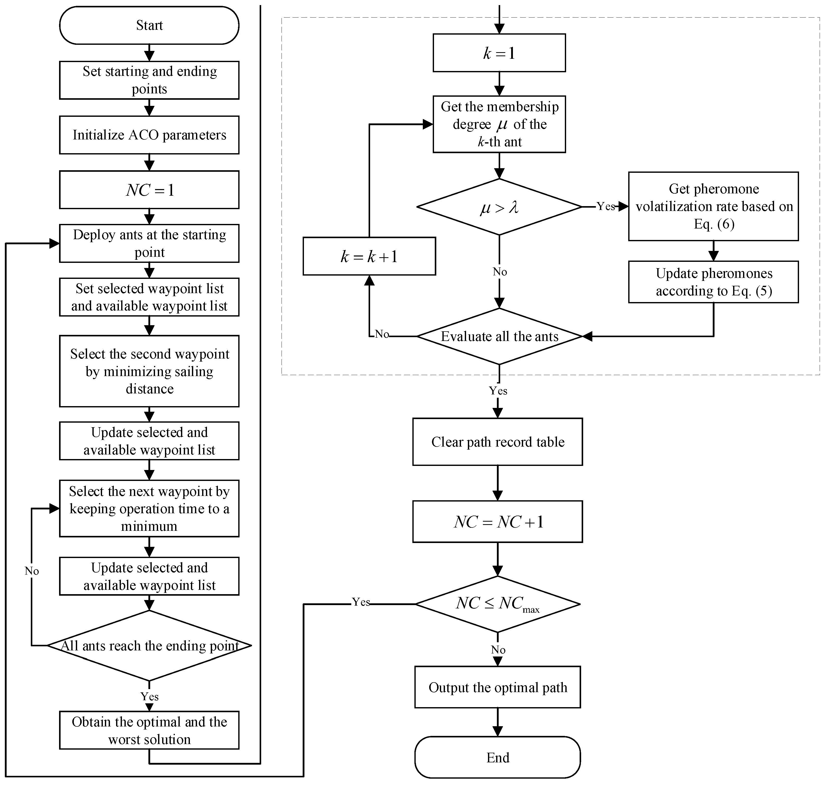
4.3. Algorithm Development Process

The improved ACO algorithm involves the following steps:

Step 1: Initialize parameters. Set starting and ending points of a navigation route, and select values for the maximum number of iterations $N{C}_{max}$, the number of ants m, the pheromone factor $\alpha$, the heuristic factor $\beta$, the measure of membership degree $\lambda$, the initial value of the pheromone volatilization coefficient ${\rho }_0$, the maximum value of pheromone volatilization coefficient ${\rho }_{max}$, the total amount of released pheromone Q in a complete traversal of a path and the pheromone amplification coefficient K.

Step 2: Construct the solution space. When located at starting point s, the probability of choosing the second waypoint for the k-th $(k=1,2,\cdots ,m)$ ant is calculated by Equation (7). The orientation of selection tends to be the shortest distance. The remaining waypoints are determined according to Equation (8) based on the shortest sailing time:

$$P_{sh}^k=\left\{\begin{array}{c}\frac{{\left[{\tau }_{sh}^d\right]}^{\alpha }{\left[{\eta }_{sh}^d\right]}^{\beta }}{{\displaystyle \sum _{h\in allo{w}_k}}{\left[{\tau }_{sh}^d\right]}^{\alpha }{\left[{\eta }_{sh}^d\right]}^{\beta }},h\in allo{w}_k;\hfill \\ 0,h\notin allo{w}_k,\hfill \end{array}\right.$$

(7)

$$P_{ijz}^k=\left\{\begin{array}{c}\frac{{\left[{\tau }_{ijz}^t\left(t\right)\right]}^{\alpha }{\left[{\eta }_{ijz}^t\left(t\right)\right]}^{\beta }}{{\displaystyle \sum _{z\in allo{w}_k}}{\left[{\tau }_{ijz}^t\left(t\right)\right]}^{\alpha }{\left[{\eta }_{ijz}^t\left(t\right)\right]}^{\beta }},z\in allo{w}_k;\hfill \\ 0,z\notin allo{w}_k,\hfill \end{array}\right.$$

(8)

where ${\tau }_{sh}^d$ is the pheromone concentration restricted by distance on a connecting path from the starting point to the second point; ${\eta }_{sh}^d$ is the corresponding distance heuristic function; ${\tau }_{ijz}^t\left(t\right)$ is the pheromone concentration constrained by operation time on a polyline path consisting of remaining points, which is the same as that in Equation (5); and ${\eta }_{ijz}^t\left(t\right)$ is the related time heuristic function.

Step 3: Update pheromone. After each ant reaches the destination, its travel time through the path is calculated, and the best and worst solutions are also recorded. Then, each ant calculates and updates membership degree $\mu \left(k\right)$, pheromone volatilization rate $\rho$ and pheromone concentration ${\tau }_{ijz}^t\left(t\right)$ according to Equations (3), (6) and (5), respectively.

Step 4: Termination judgment. If $NC<N{C}_{max}$, let $NC=NC+1$, clear the path record table and return to Step 2. Otherwise, the loop ends, and the optimal solution is yielded.

A flow chart of our proposed algorithm is shown in Figure 3.

The pseudo-code of our proposed Algorithm 1 is presented as follows:

Algorithm 1 Improved ant colony algorithm.

1: Enter the coordinate of n target points for further exploration; 2: Initialize parameters $N{C}_{max}$, m, $\alpha$, $\beta$, $\lambda$, ${\rho }_0$, ${\rho }_{max}$, Q, K; 3: Initialize ${\tau }_{sh}^d$, ${\eta }_{sh}^d$, ${\tau }_{ijz}^t\left(t\right)$, ${\eta }_{ijz}^t\left(t\right)$ by the inverse of distance and operation time; 4: Select starting point s and ending point e from suspected target points; 5: Set $NC=1$; 6: while$NC\le N{C}_{max}$do 7:    for each $k\in [1,m]$ do 8:      $rout{e}_{Ant\left(k\right)}(k,1)=s$; /*Establish a table $rout{e}_{Ant\left(k\right)}$ to record the selected waypoints for all ants*/ 9:      $rout{e}_{Ant\left(k\right)}(k,n)=e$; 10:      Add s to $tab{u}_{Ant\left(k\right)}$; /*Establish a tabu list $tab{u}_{Ant\left(k\right)}$ for the k-th ant and add starting and ending points to $tab{u}_{Ant\left(k\right)}$*/ 11:      Add e to $tab{u}_{Ant\left(k\right)}$; 12:      Create a list of target points to be accessed $\left(Allowe{d}_{Ant\left(k\right)}\right)$ based on $tab{u}_{Ant\left(k\right)}$; 13:      $sec=select\_second\_node\left(Allowe{d}_{Ant\left(k\right)}\right)$; /*Identify the second point by Equation (7)*/ 14:      $rout{e}_{Ant\left(k\right)}(k,2)=sec$; 15:      Add $sec$ to $tab{u}_{Ant\left(k\right)}$; 16:      Update $Allowe{d}_{Ant\left(k\right)}$ based on $tab{u}_{Ant\left(k\right)}$; 17:      for each $h\in [3,n-1]$ do 18:         $nex=select\_next\_node\left(Allowe{d}_{Ant\left(k\right)}\right)$; /*Choose the next point from $Allowe{d}_{Ant\left(k\right)}$ by Equation (8) */ 19:         $rout{e}_{Ant\left(k\right)}(k,h)=nex$; 20:         Add $nex$ to $tab{u}_{Ant\left(k\right)}$; 21:         Update $Allowe{d}_{Ant\left(k\right)}$ based on $tab{u}_{Ant\left(k\right)}$; 22:      end for 23:      Clear $tab{u}_{Ant\left(k\right)}$; 24:    end for 25:    Calculate the operation time T it takes for an ant to traverse a path; 26:    for each $k\in [1,m]$ do 27:      Calculate membership degree $\mu \left(k\right)$ for the k-th ant by Equation (3); 28:      if $\mu \left(k\right)>\lambda$ then 29:         Calculate dynamic pheromone evaporation rate $\rho$ by Equation (6); 30:         for each $j\in [2,n-1]$ do 31:           $i=j-1$; $z=j+1$; 32:           Update pheromone ${\tau }_{ijz}^t\left(t\right)$ on path segment $(i,j,z)$ by Equation (5) in the way that condition holds; 33:           Update pheromone ${\tau }_{ijz}^t\left(t\right)$ on path segment $(i,j,z+1:n-1)$ by Equation (5) according to the counter case; 34:         end for 35:      end if 36:    end for 37:    $NC=NC+1$; 38:    Clear $rout{e}_{Ant\left(k\right)}$; 39: end while

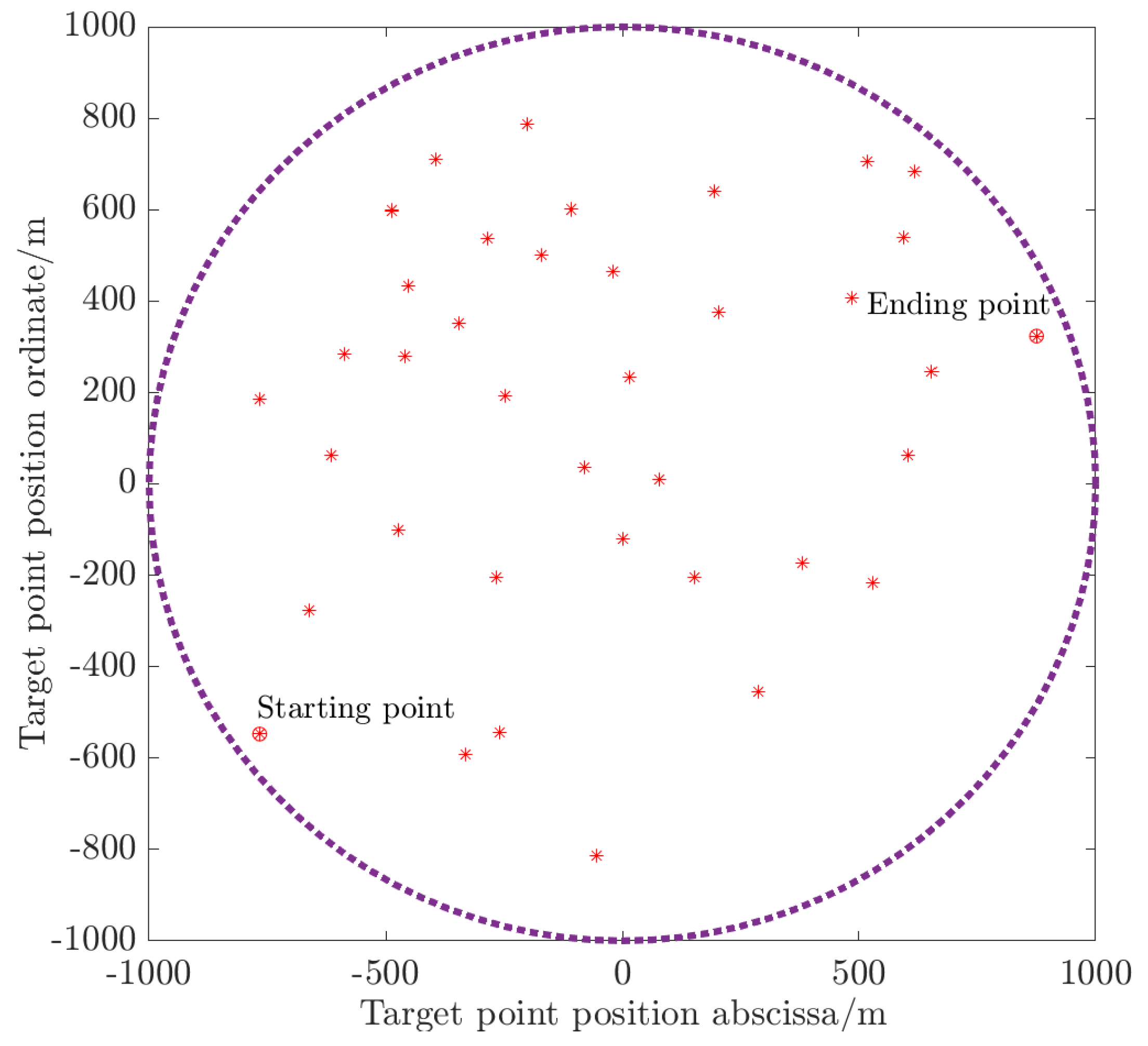
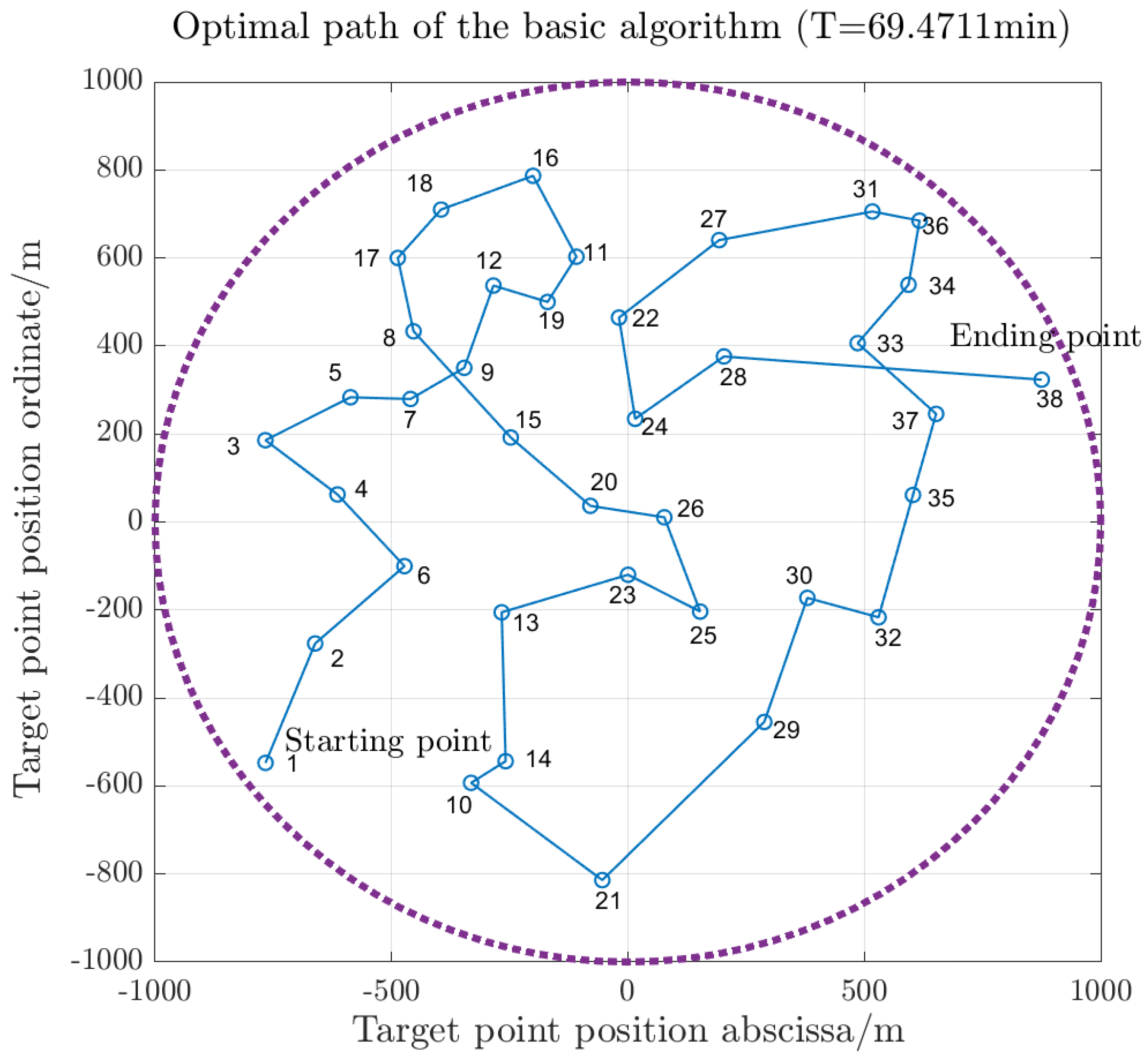
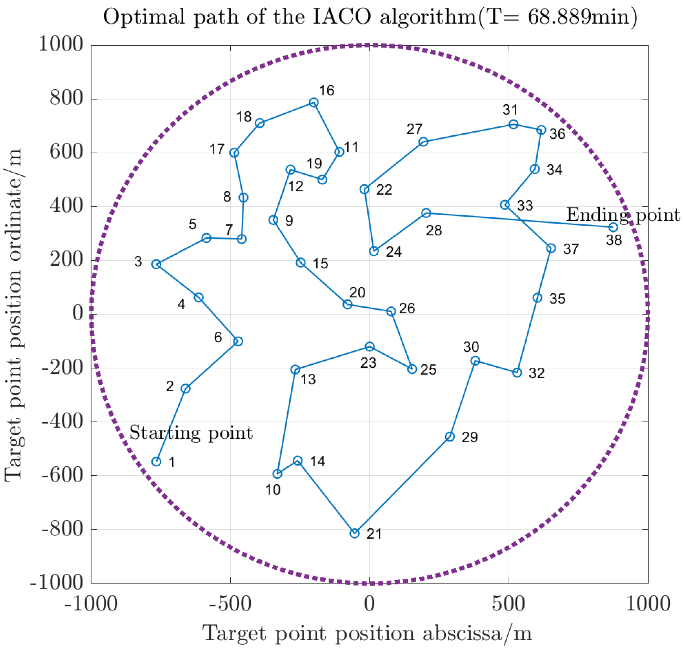
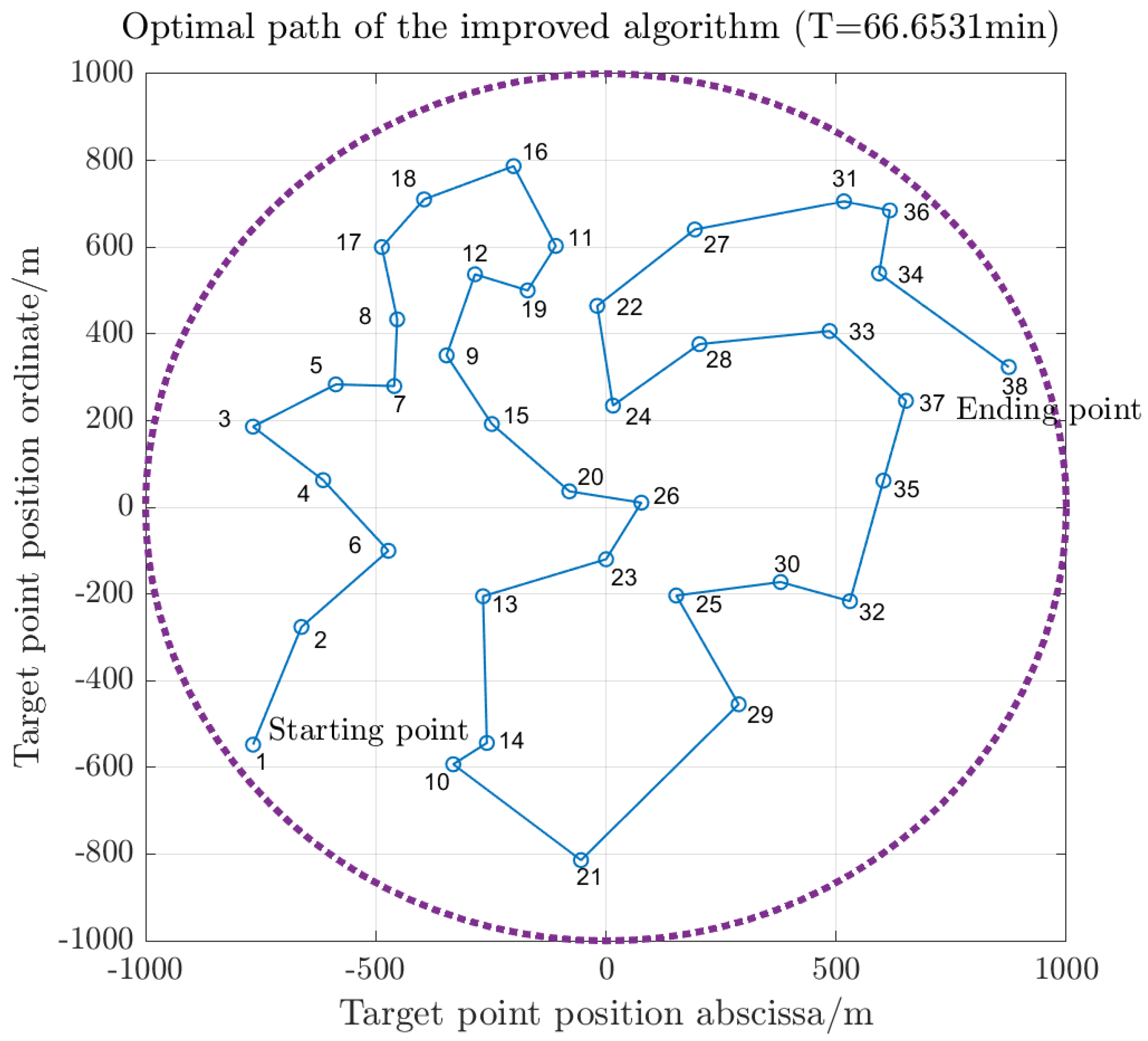
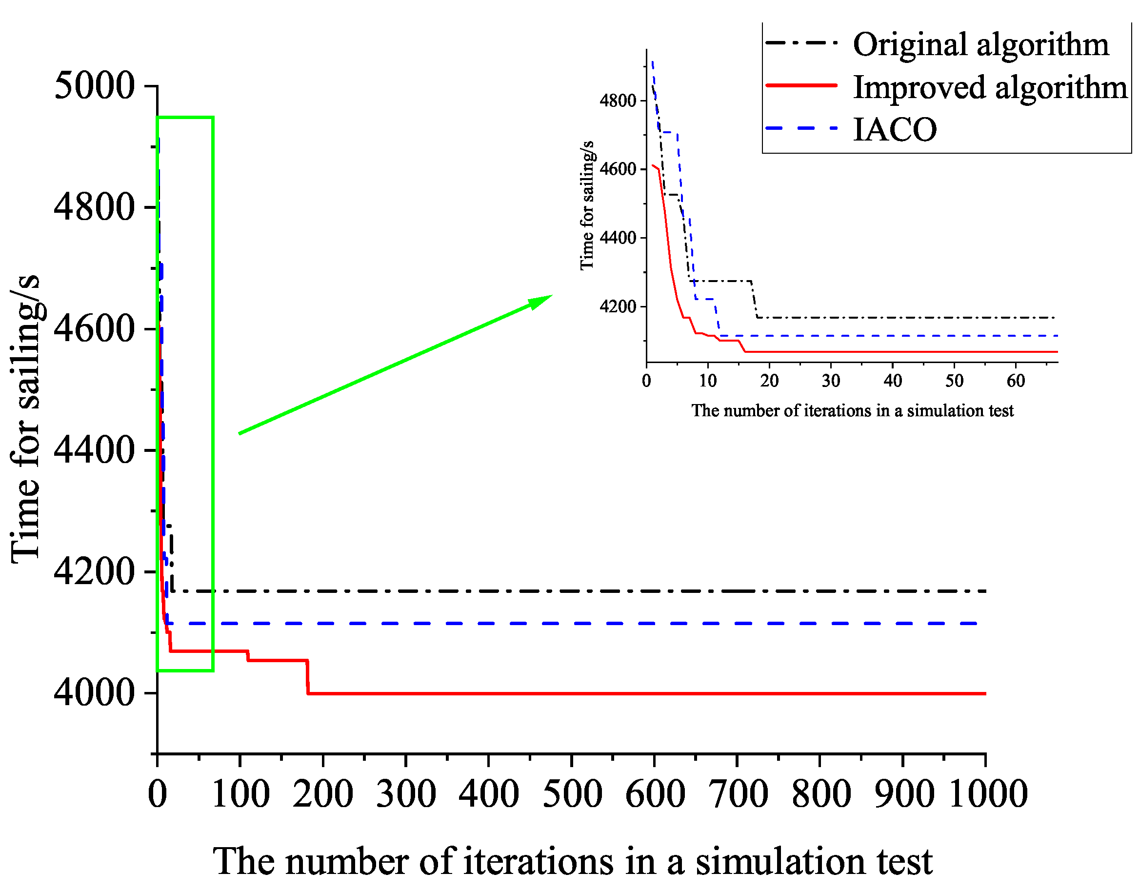
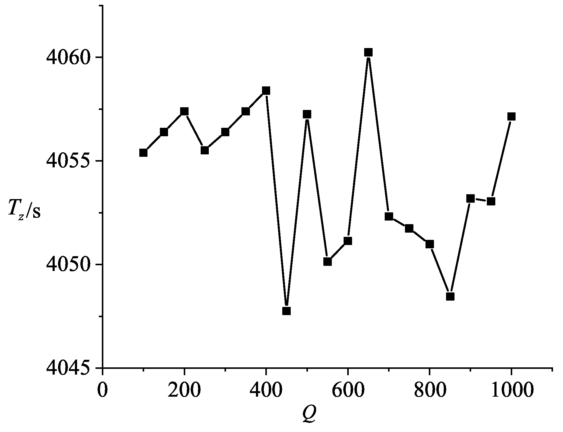
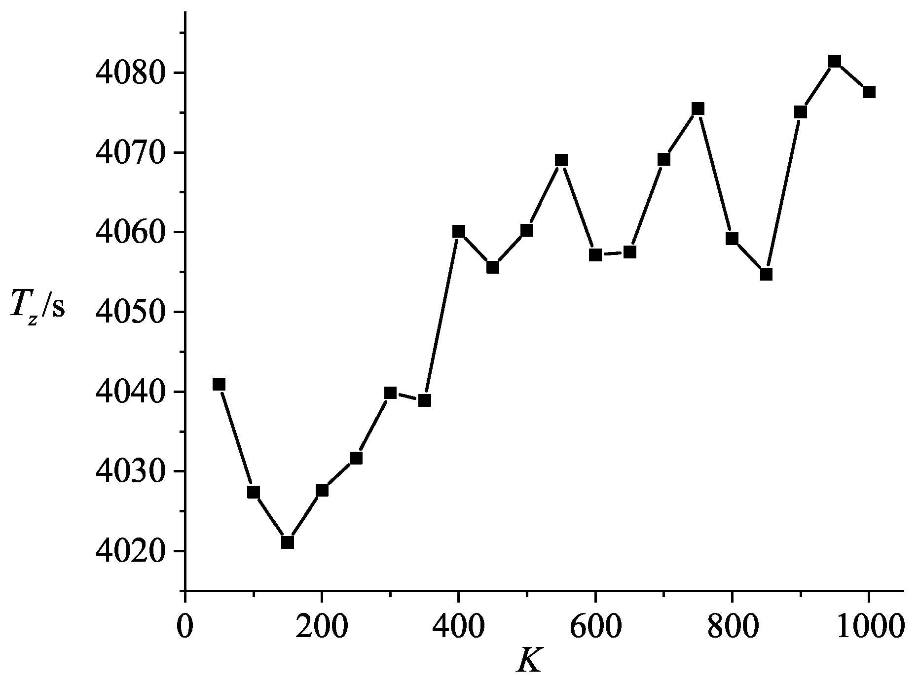
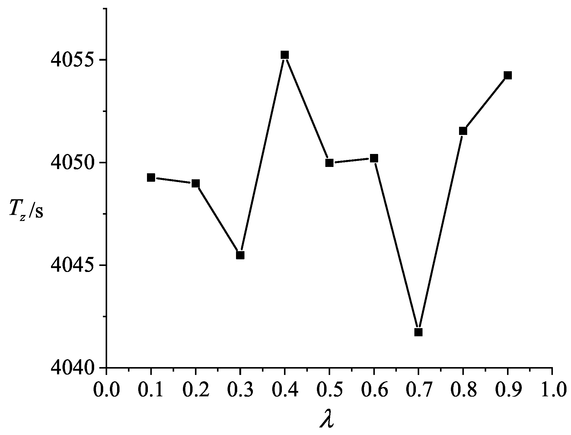
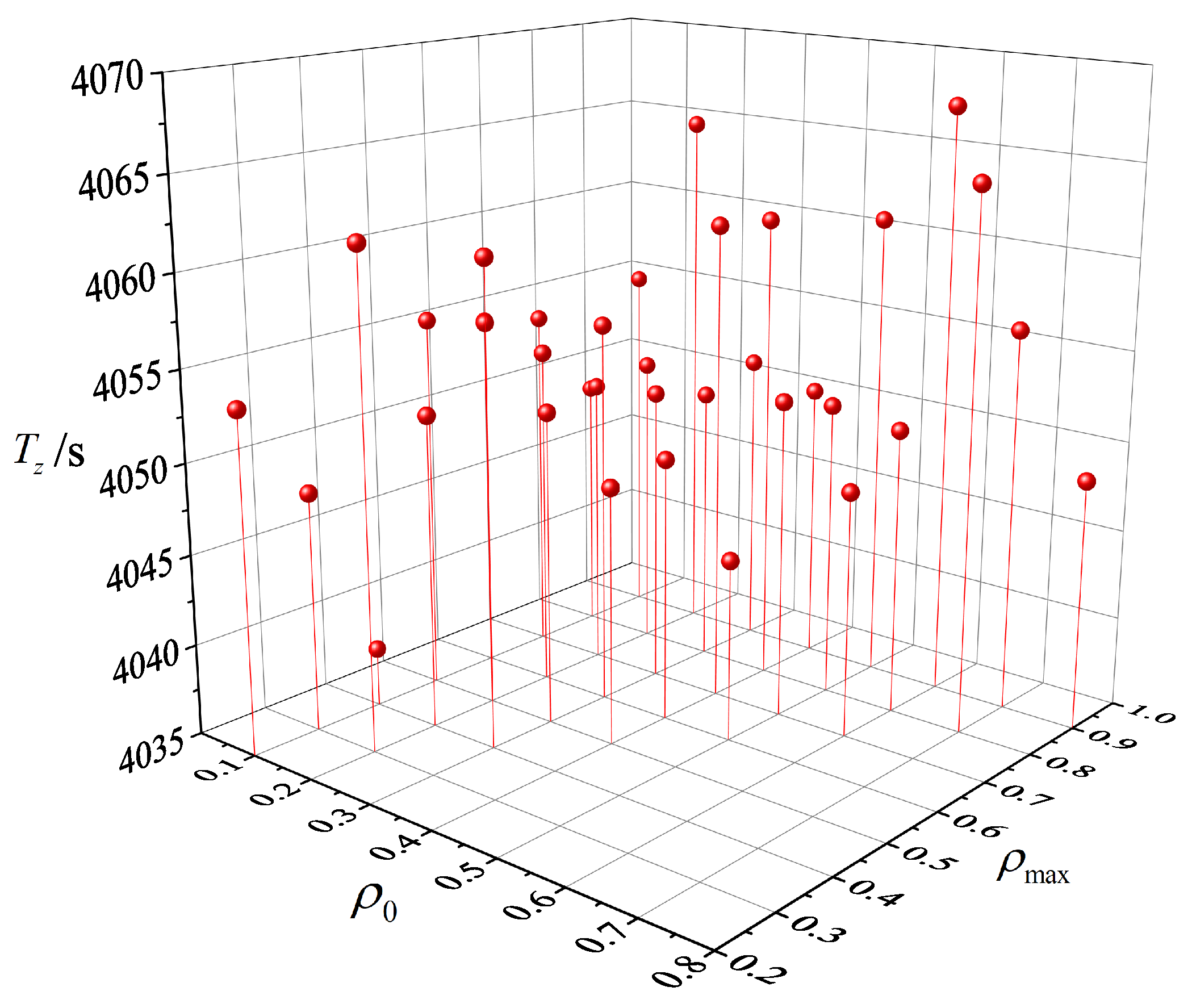
5. Simulation Results and Analysis

In this section, an example is provided to validate the feasibility and effectiveness of the improved ACO algorithm. The effect of the improved algorithm is compared with that of the original ant colony algorithm and the IACO algorithm in [39]. In a scenario where an AUV and an unmanned surface vehicle (USV) cooperate to detect underwater high-risk targets, it is assumed that the USV has found 36 suspected targets in a circular area with a radius of 1000 m, as shown in Figure 4. The AUV is arranged to sail closer to each target for fine-grained recognition and verification. The cruise speed $v_1$ of the AUV is 4 kn, and the turning speed $v_2$ is 3 kn.

Matlab2021b is employed to validate the scheduling algorithms, running on a computer with an Intel Core i5-7200U and 12 GB of RAM. The configuration of experimental parameters of the original ACO algorithm, the IACO algorithm and the improved ACO algorithm are presented in

Table 1. Parameter settings of the ACO algorithm.

Parameter	Value
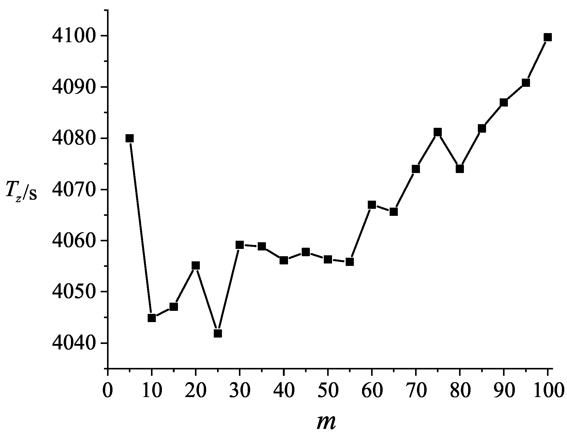
Number of ants m	33
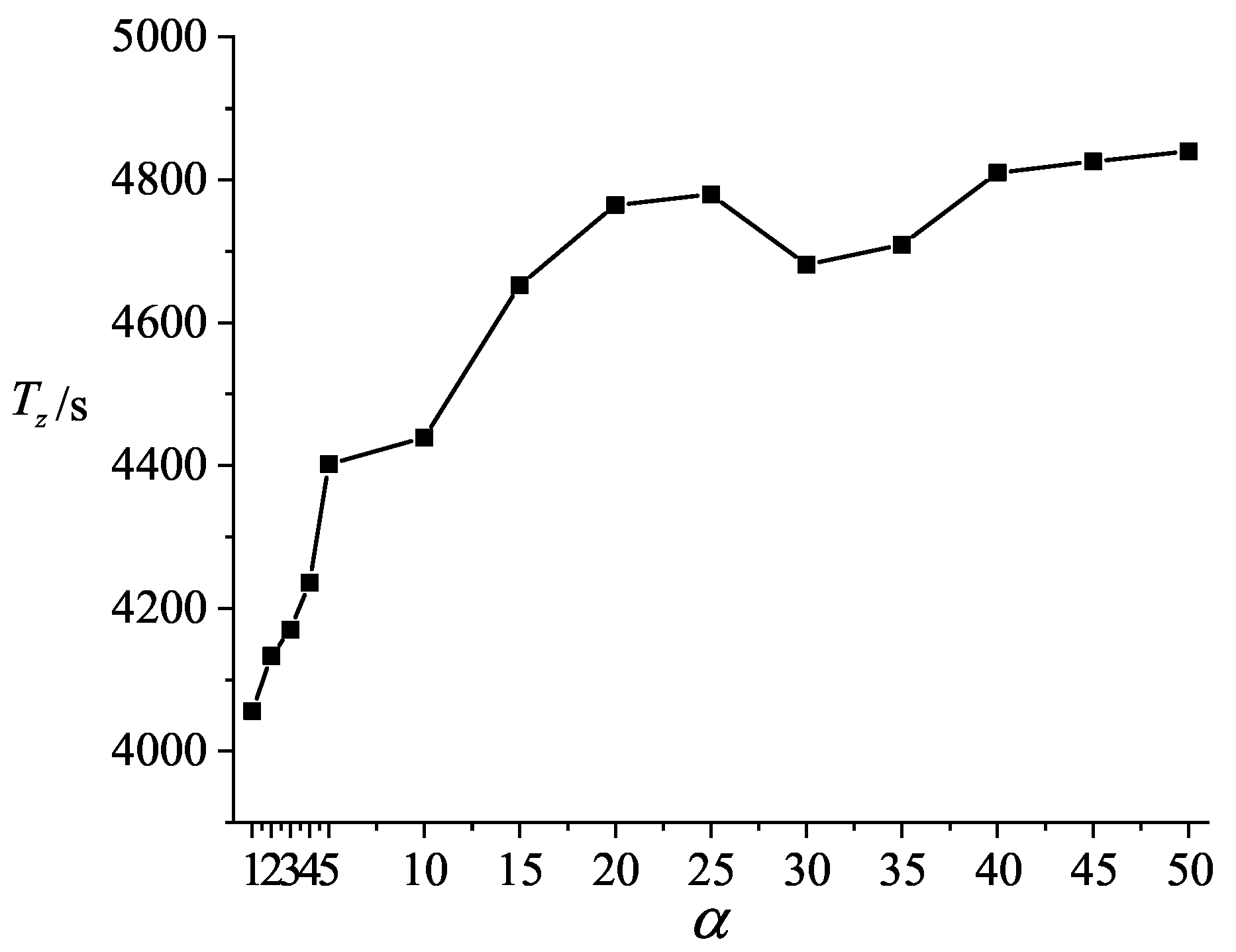
Pheromone weight $\alpha$	1
Inspired information weight $\beta$	5
Pheromone evaporation coefficient $\rho$	0.2
Total amount of pheromone Q	300
Maximum number of iterations $N{C}_{max}$	1000

,

Table 2. Parameter settings of the IACO algorithm.

Parameter	Value
Number of ants m	33
Pheromone weight $\alpha$	1
Inspired information weight $\beta$	5
Pheromone evaporation coefficient $\rho$	0.55
Total amount of pheromone Q	300
Maximum number of iterations $N{C}_{max}$	1000

and

Table 3. Parameter settings of our proposed ACO algorithm.

Parameter	Value
Number of ants m	33
Pheromone weight $\alpha$	1
Inspired information weight $\beta$	5
Measure of membership degree $\lambda$	0.6
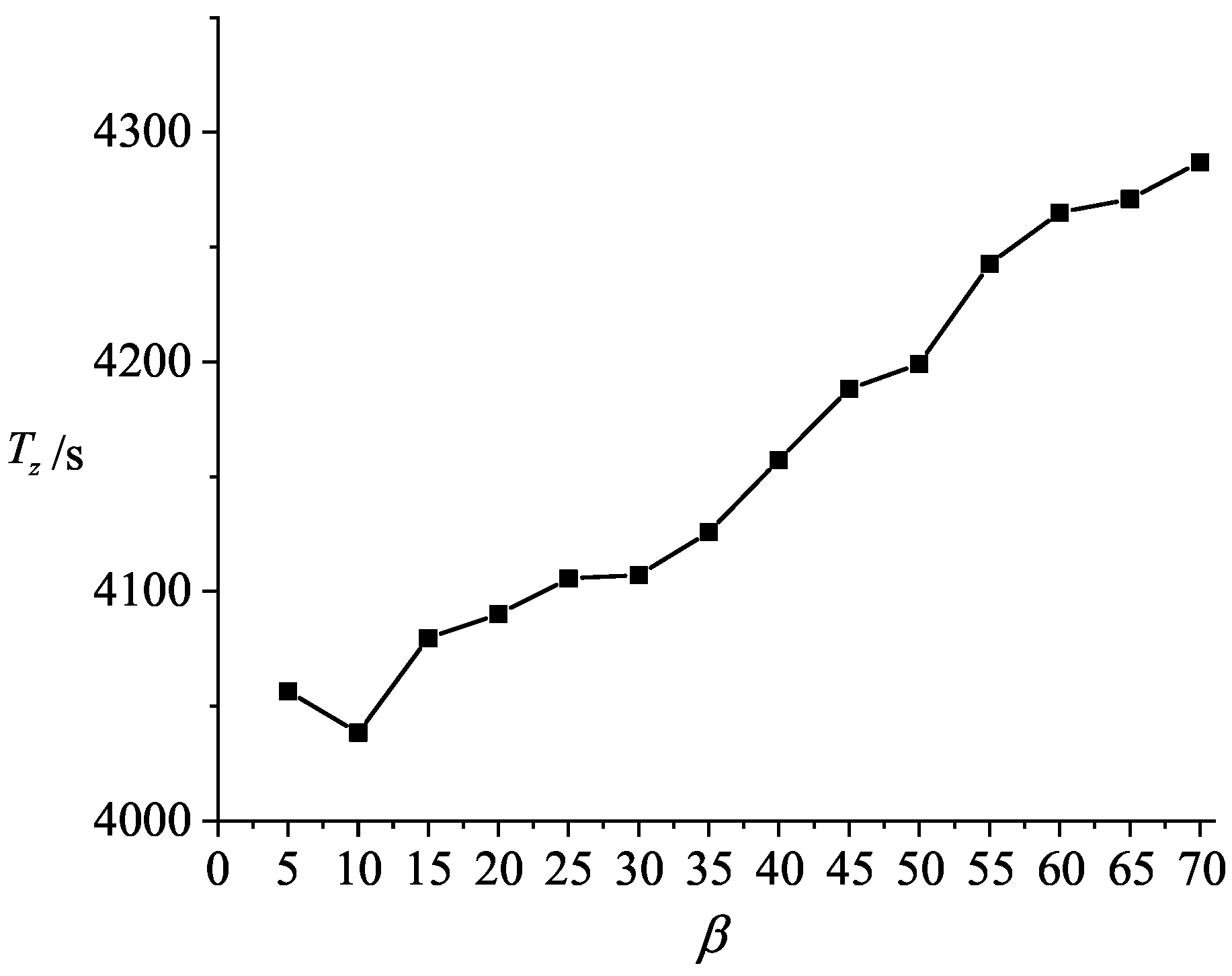
Initial pheromone volatilization coefficient ${\rho }_0$	0.2
Maximum pheromone volatilization coefficient ${\rho }_{max}$	0.5
Total amount of pheromone Q	300
Maximum number of iterations $N{C}_{max}$	1000
Pheromone amplification coefficient K	20

, respectively.

Table 4. Statistical results of T obtained by running the simulation 50 times.

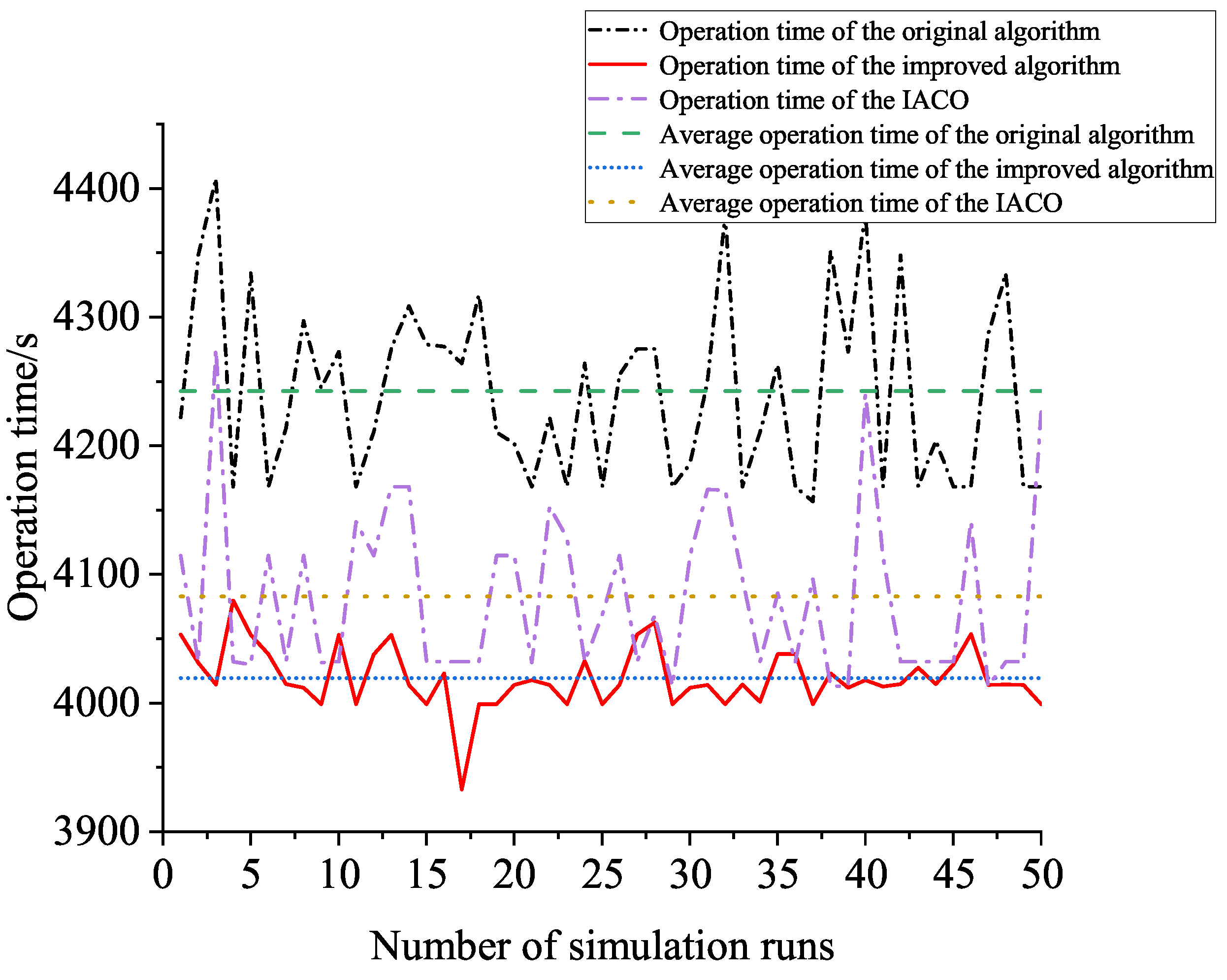
Algorithm	Minimum Duration/s	Average Duration/s	Maximum Duration/s
Original ACO	4156.9214	4242.7417	4407.9726
IACO	4013.1685	4083.0390	4275.2756
Improved ACO	3932.9216	4019.6800	4079.8440

reveals the comparison results of 50 simulation runs on operation time T of three algorithms. As can be seen from Table 4, the improved ACO algorithm enhances the ability of finding the optimal solution to some extent. Based on the statistical results of the 50 simulated sets, the improved algorithm achieves 5.4%, 5.3% and 7.4% greater time length reductions in terms of the minimum, average and maximum values, respectively, compared with the basic algorithm. In comparison with the IACO algorithm, the improved algorithm achieves 2%, 1.6% and 4.6% greater time length reductions in terms of the minimum, average and maximum values, respectively. From Figure 5, we observe that operation time varies within a small amplitude range, which demonstrates that the improved algorithm has better stability performance than the original algorithm and the IACO algorithm.

Figure 6, Figure 7 and Figure 8 are optimal paths obtained after 50 simulation tests, which are produced by the basic algorithm, the IACO algorithm and the improved algorithm, respectively. Figure 8 intuitively demonstrates the superiority of the improved algorithm. The produced path not only makes AUV’s cruising time shorter than the original algorithm and the IACO algorithm, but it also ensures as many acute rotation angles as possible, which is more in line with maneuvering characteristics of an AUV.

Figure 9 describes the corresponding relationship between the number of iterations $NC$ and operation time T in a simulation test, reflecting the convergence property of the algorithm. It is easy to see that the improved algorithm converges much more quickly than the original algorithm and the IACO algorithm at earlier stages in the iteration. As the iteration process progresses, the search for a solution with the lowest path cost among all feasible solutions is continuing, and the problem of the optimization process becoming trapped at a local optimum is avoided. Obtaining such satisfactory results is entirely due to the development of a pheromone update rule. In early iterations of the algorithm, the modified update rule enables a rapid accumulation of pheromones on the preferred path, which strengthens search orientation and encourages subsequent ants to assemble towards the preferred path. In later phases of iterations, the modified update rule weakens the positive guiding effects in the search direction in order to increase the global search ability of the algorithm.

In the following content, we will analyze and discuss the issue of parameter settings in our proposed algorithm. Except for parameters to be analyzed, the settings of other parameters are consistent with those in Table 3. A total of 20 simulations are conducted, and the average of the simulation results is regarded as the final result. Define total time $T_z$ as $T_z=T_c+T$, where $T_c$ is the running time of the algorithm. The curve in Figure 10 depicts the relationship between total time $T_z$ and ant population m. The number of ants corresponding to the lowest total time is 25. We can also see from Figure 10 that the increase in the number of ants provides a boost in the global search capacity of the algorithm. However, an excessive increase does not provide much assistance in the improvement of the optimization ability of the algorithm; instead, it makes the computational resource consumption higher and the total time longer.

Figure 11 presents a variation curve of total time $T_z$ and heuristic pheromone weight $\beta$. Regarding $\beta$, the recommended value is 10. A smaller value of $\beta$ leads ants to becoming trapped in random search decisions, while a larger value of $\beta$ causes the algorithm to become stuck with a local optimal solution.

A variation curve of total time $T_z$ with respect to pheromone weight $\alpha$ is given in Figure 12. It can be seen that with the increase in $\alpha$, the $T_z$ presents an upward trend. The reason is that the larger $\alpha$ is, the greater the probability that the ant will choose the path it traveled before, which makes the search less random. Taking the data in Figure 12 as a reference, it is more appropriate to set $\alpha$ to 1.

In Figure 13, the relationship between total time $T_z$ and total pheromone concentration Q is revealed. Obviously, the scale of the optimization problem, that is, the number of potential targets, is a key factor affecting the value of Q. Here, we recommend a Q value of 450.

In Figure 14, the interaction between pheromone amplification factor K and total time $T_z$ is investigated. For K, a value of 150 is assigned.

Figure 15 gives a changing curve of total time $T_z$ with respect to the evaluation parameter of membership degree $\lambda$. If the value of $\lambda$ is too small, then the solution is more conservative. If the value of $\lambda$ is too large, then the number of better paths that can be selected as the preferred path in one iteration is not sufficient, accelerating the tendency of the algorithm to fall into local optima. For $\lambda$, the suggested setting is 0.7.

Then, Figure 16 provides a reference value for pheromone volatilization loss rate $\rho$. When the maximum value and the initial value of the pheromone evaporation rate are set to 0.4 and 0.1, respectively, the algorithm has a strong global search ability.

6. Conclusions

In this paper, an improved ACO algorithm is proposed to assist an AUV that is performing a multiple-target search mission to address the autonomous task allocation problem. The actual problem is reducible to a multi-objective TSP which encompasses the optimization of distance-associated and turning-angle-dependent objectives. In order to improve the performance of the original algorithm for solving the optimization problem, a membership function and a dynamic pheromone volatilization rule are developed. With the help of the membership function, the better and worse paths are clearly distinguished, which provides convenient conditions for realizing that pheromone is only updated on better paths, thereby enhancing pathfinding guidance in the early stage of the ACO algorithm. By means of the dynamic pheromone volatilization rule, more pheromones are volatilized on better paths as the number of iterations of the ACO algorithm increases, thus providing the algorithm with a solution to overcome local minima in the later stage. Futhermore, the article elaborates on the effects of parameter variation on algorithm performance. A viable extension of this work could be to multi-AUV task scheduling problems. Further investigations will focus on issues of the fairness of task distribution, the incommensurability among objectives and solution evaluation methods.

References

- Wang, G.; Wei, F.; Jiang, Y.; Zhao, M.; Wang, K.; Qi, H. A Multi-AUV Maritime Target Search Method for Moving and Invisible Objects Based on Multi-Agent Deep Reinforcement Learning. Sensors 2022, 22, 8562. [Google Scholar] [CrossRef]
- Li, J.; Li, C.; Chen, T.; Zhang, Y. Improved RRT Algorithm for AUV Target Search in Unknown 3D Environment. J. Mar. Sci. Eng. 2022, 10, 826. [Google Scholar] [CrossRef]
- Liu, H.; Xu, B.; Liu, B. An Automatic Search and Energy-Saving Continuous Tracking Algorithm for Underwater Targets Based on Prediction and Neural Network. J. Mar. Sci. Eng. 2022, 10, 283. [Google Scholar] [CrossRef]
- Gan, W.; Zhu, D.; Ji, D. QPSO-model predictive control-based approach to dynamic trajectory tracking control for unmanned underwater vehicles. Ocean Eng. 2018, 158, 208–220. [Google Scholar] [CrossRef]
- Kang, J.; Kim, T.; Kwon, L.; Kim, H.; Park, J. Design and Implementation of a UUV Tracking Algorithm for a USV. Drones 2022, 6, 66. [Google Scholar] [CrossRef]
- Liang, X.; Qu, X.; Hou, Y.; Li, Y.; Zhang, R. Finite-time unknown observer based coordinated path-following control of unmanned underwater vehicles. J. Frankl. Inst. 2021, 258, 2703–2721. [Google Scholar] [CrossRef]
- Peng, F.; Wang, Y.; Xuan, H.; Nguyen, T. Efficient road traffic anti-collision warning system based on fuzzy nonlinear programming. Int. J. Syst. Assur. Eng. Manag. 2022, 13, 456–461. [Google Scholar] [CrossRef]
- Wang, C.; Yang, F.; Vo, N.; Nguyen, V. Wireless Communications for Data Security: Efficiency Assessment of Cybersecurity Industry & mdash; A Promising Application for UAVs. Drones 2022, 6, 363. [Google Scholar]
- Ding, W.; Cao, H.; Gao, H.; Ma, Y.; Mao, Z. Investigation on optimal path for submarine search by an unmanned underwater vehicle - sciencedirect. Comput. Electr. Eng. 2019, 79, 106468. [Google Scholar] [CrossRef]
- Zhao, Y.; Xing, W.; Yuan, H.; Shi, P. A collaborative control framework with multi-leaders for AUVs based on unscented particle filter. J. Frankl. Inst. 2016, 353, 657–669. [Google Scholar] [CrossRef]
- Kragelund, S.; Walton, C.; Kaminer, I.; Dobrokhodov, V. Generalized optimal control for autonomous mine countermeasures missions. IEEE J. Ocean. Eng. 2020, 46, 466–496. [Google Scholar] [CrossRef]
- Yuan, S.; Chen, K.; Li, J.; Zhang, P. Exact algorithms for the min-max cycle cover problem. Sci. Sin. Inf. 2022, 52, 960–970. [Google Scholar] [CrossRef]
- Ghalami, L.; Grosu, D. Scheduling parallel identical machines to minimize makespan:a parallel approximation algorithm. J. Parallel Distrib. Comput. 2019, 133, 221–231. [Google Scholar] [CrossRef]
- Liu, L.; Zhang, H.; Xie, J.; Zhao, Q. Dynamic Evacuation Planning on Cruise Ships Based on an Improved Ant Colony System (IACS). J. Mar. Sci. Eng. 2021, 9, 220. [Google Scholar] [CrossRef]
- Skinderowicz, R. Improving Ant Colony Optimization Efficiency for Solving Large TSP Instances. Appl. Soft Comput. 2022, 120, 10865. [Google Scholar] [CrossRef]
- Yu, J.; You, X.; Liu, S. Dynamically induced clustering ant colony algorithm based on a coevolutionary chain. Knowl.-Based Syst. 2022, 251, 109231. [Google Scholar] [CrossRef]
- Alipour, M.; Razavi, S.; Feizi Derakhshi, M.; Balafar, M. A hybrid algorithm using a genetic algorithm and multiagent reinforcement learning heuristic to solve the traveling salesman problem. Neural Comput. Appl. 2018, 30, 2935–2951. [Google Scholar] [CrossRef]
- Zheng, Y.; Lv, X.; Qian, L.; Liu, X. An Optimal BP Neural Network Track Prediction Method Based on a GA-ACO Hybrid Algorithm. J. Mar. Sci. Eng. 2022, 10, 1399. [Google Scholar] [CrossRef]
- Zhou, H.; Song, M.; Pedrycz, W. A comparative study of improved ga and pso in solving multiple traveling salesmen problem. Appl. Soft Comput. J. 2018, 64, 564–580. [Google Scholar] [CrossRef]
- Qiao, S.; Lv, Z.; Zhang, N. Improved particle swarm optimization algorithm based on hamming distance for traveling salesman problem. J. Comput. Appl. 2017, 37, 2767–2772. [Google Scholar]
- Zheng, Q.; Feng, B.; Liu, Z.; Chang, H. Application of Improved Particle Swarm Optimisation Algorithm in Hull form Optimisation. J. Mar. Sci. Eng. 2021, 9, 955. [Google Scholar] [CrossRef]
- Zhong, Y.; Lin, J.; Wang, L.; Zhang, H. Discrete comprehensive learning particle swarm optimization algorithm with metropolis acceptance criterion for traveling salesman problem. Swarm Evol. Comput. 2018, 42, 77–88. [Google Scholar] [CrossRef]
- Wang, C.; Yang, F.; Nguyen, V.; Vo, N. CFD Analysis and Optimum Design for a Centrifugal Pump Using an Effectively Artificial Intelligent Algorithm. Micromachines 2022, 13, 1208. [Google Scholar] [CrossRef] [PubMed]
- Zhou, X.; Huang, X.; Zhao, X. Optimization of the critical slip surface of three-dimensional slope by using an improved genetic algorithm. Int. J. Geomech. 2020, 20, 1–8. [Google Scholar] [CrossRef]
- Zheng, K.; Yuan, X.; Xu, Q.; Dong, L.; Yan, B.; Chen, K. Hybrid particle swarm optimizer with fitness-distance balance and individual self-exploitation strategies for numerical optimization problems. Inf. Sci. 2022, 608, 424–452. [Google Scholar] [CrossRef]
- Zhang, S.; Pu, J.; Si, Y.; Sun, L. Survey on application of ant colony algorithm in path planning of mobile robot. Comput. Eng. Appl. 2020, 56, 10–19. [Google Scholar]
- Ye, K.; Zhang, C.; Ning, J.; Liu, X. Ant-colony algorithm with a strengthened negative-feedback mechanism for constraint-satisfaction problems. Inf. Sci. 2017, 406, 29–41. [Google Scholar] [CrossRef]
- Yang, J.; Ding, R.; Zhang, Y.; Cong, M.; Wang, F.; Tang, G. An improved ant colony optimization (i-aco) method for the quasi travelling salesman problem (quasi-tsp). Int. J. Geogr. Inf. Sci. 2015, 29, 1534–1551. [Google Scholar] [CrossRef]
- Yang, K.; You, X.; Liu, S.; Pan, H. A novel ant colony optimization based on game for traveling salesman problem. Appl. Intell. 2020, 50, 4529–4542. [Google Scholar] [CrossRef]
- Ebadinezhad, S. DEACO: Adopting dynamic evaporation strategy to enhance ACO algorithm for the traveling salesman problem. Eng. Appl. Artif. Intell. 2020, 92, 103649. [Google Scholar] [CrossRef]
- Li, Z.; Huang, Y.; Xu, Y. Path planning of mobile robot based on improved variable step size ant colony algorithm. J. Electron. Meas. Instrum. 2020, 32, 7. [Google Scholar]
- Zhang, Q.; Zhang, C. An improved ant colony optimization algorithm with strengthened pheromone updating mechanism for constraint satisfaction problem. Neural Comput. Appl. 2018, 30, 3209–3220. [Google Scholar] [CrossRef]
- Yi, N.; Xu, J.; Yan, L.; Huang, L. Task optimization and scheduling of distributed cyber–physical system based on improved ant colony algorithm. Future Gener. Comput. Syst. 2020, 109, 134–148. [Google Scholar] [CrossRef]
- Chen, D.; You, X.; Liu, S. Ant colony algorithm with Stackelberg game and multi-strategy fusion. Appl. Intell. 2022, 52, 6552–6574. [Google Scholar] [CrossRef]
- Wu, Y.; Ma, W.; Miao, Q.; Wang, S. Multimodal continuous ant colony optimization for multisensor remote sensing image registration with local search. Swarm Evol. Comput. 2019, 47, 89–95. [Google Scholar] [CrossRef]
- Deng, W.; Zhang, L.; Zhou, X.; Zhou, Y.; Sun, Y.; Zhu, W.; Chen, H.; Deng, W.; Chen, H.; Zhao, H. Multi-strategy particle swarm and ant colony hybrid optimization for airport taxiway planning problem. Inf. Sci. 2022, 612, 576–593. [Google Scholar] [CrossRef]
- Zhang, H.; Zhang, Q.; Ma, L.; Zhang, Z.; Liu, Y. A hybrid ant colony optimization algorithm for a multi-objective vehicle routing problem with flexible time windows. Inf. Sci. 2019, 490, 166–190. [Google Scholar] [CrossRef]
- Zhao, H.; Zhang, C.; Zhang, B. A decomposition-based many-objective ant colony optimization algorithm with adaptive reference points. Inf. Sci. 2020, 540, 435–448. [Google Scholar] [CrossRef]
- Zhang, Y.; Ding, X.; Xue, D.; Wang, X. An improved ant colony algorithm for traveling salesman problem. Comput. Eng. Sci. 2017, 39, 1576–1580. [Google Scholar]