A Frequency-Dependent Assimilation Algorithm: Ensemble Optimal Smoothing

Abstract

Motivated by the need for a simple and effective assimilation scheme that could be used in a relocatable ocean model, a new assimilation algorithm called ensemble optimal smoothing (EnOS) was developed. This scheme was a straightforward extension of the ensemble optimal interpolation (EnOI) by involving time correlation information in the Kalman gain. The main advantage of this scheme was the ability to estimate the present state from the time history of observation. We first examined the new scheme in an ideal ocean model using simulated observations. Further applying these two assimilation schemes to the Chinese offshore and adjacent waters, the root-mean-square error (RMSE) of the EnOS scheme was reduced by 6.4% relative to EnOI. The results showed that the EnOS was more efficient and effective in eliminating model errors when compared to the EnOI scheme.

1. Introduction

The tasks of reconstructing the past and also predicting future states have been emphasized in oceanographic research in recent decades. An important aspect of ocean reanalysis and forecast is data assimilation, in which observations are combined with a model background field to generate an optimal initial condition [1,2,3]. The theory of data assimilation can be well described in a Bayesian framework [4]. One of the most sophisticated schemes is the particle filter/smoother, which approximates the density of the state conditioned on the observations by an ensemble of “particles” that can be considered the realizations of the density [5]. Another class of solutions is the development of assimilation methods based on the Kalman filter; for example, a fully extended Kalman filter requires a large number of model calculations and is therefore not ideal for application in efficient numerical ocean model forecasting.

Ensemble Kalman filters(EnKF) and smoothers provide more practical alternatives for estimating the present state of ocean models and reconstructing the past, respectively [1,2,6]. In an ensemble-based scheme, different perturbation models are used to construct the ensemble samples and thus obtain the background covariance matrix, which is the key part of the Kalman filter scheme. Since an EnKF is sensitive to the ensemble number when the ensemble size is limited [7,8,9], the operation of such a method is still limited by the computational requirements. In practice, many operational models; for example, HYCOM and NEMO, still use suboptimal and relatively simple schemes [10].

As one of the simplest schemes, EnOI is widely used to assimilate ocean observations into realistic ocean models [11,12,13]. EnOI uses information on the present time $t$ to update the present state of the system. Unlike the EnKF, which is computationally costly, the EnOI calculates the model covariance only from a single model prediction. This means the EnOI is not “flow dependent”; i.e., the covariance structure does not change with the background state [14,15,16,17]. In this study, we proposed and evaluated a straightforward extension of the EnOI to allow for the time history of the observations to estimate the present state of the ocean in a recursive fashion. This work was a simple and effective assimilation scheme that could be used in a relocatable ocean model that could be applied on a shelf where multiple time scales of variability can exist (e.g., tidal, synoptic, and intraseasonal). The development of land-based HF radar systems that are capable of measuring ocean surface currents provides enormous amounts of coastal ocean measurements. These observations contain information on tides and slow baroclinic changes, each with their own spatial covariance structures [18]. In most earlier studies on HF radar data assimilation, the tidal information was eliminated using a low-pass filter [19,20].

Our approach was motivated by computational efficiency and does not require running models backward in time or overlapping forecast runs [21,22]. The fixed lag smoother does not update the most recent state because it contains all of the info available from the observation up to the present time. This is the value we updated every $\tau$ time steps, so in that sense, it did correspond to a smoother estimate. We will show that this approach allowed the new method’s approximation of the Kalman gain to be frequency-dependent, unlike EnOI. The approach sits between EnOI and smoothing, and we will hereafter refer to it as EnOS.

This study was the first step in the implementation and evaluation of EnOS in a realistic ocean model that will be the subject of a future study. We first considered a simple, linear model of the ocean: the forced Rossby wave model in one spatial dimension [23,24]. One advantage of this simple linear dynamical model is that we can obtain analytical expressions for the skill of the various schemes [25]. It also provided insights into when and where we could expect EnOS to outperform EnOI. We next tried EnOI and EnOS schemes using real datasets. The implementation of EnOS in this setting presented a much greater challenge because the temporal and spatial scales of change varied with location, which complicated the estimation of the covariance structures for EnOS [18,26].

The structure of this paper is organized as follows. In Section 2, the assimilation methodology is described. Experiments of the scheme on idealized linear model are described in Section 3. In Section 4, single-point observation experiments are conducted using real data for current regions with different characteristics to perform sensitivity analysis of the time-dependent terms. The assimilation scheme is then implemented in the coastal waters of China and adjacent seas using multiple observation points and compared with EnOI in Section 5. In the final section, we summarize the results and also describe plans for how the new scheme will be implemented in a realistic operational ocean model.

2. Assimilation Theory

2.1. Overview of Sequential Ensemble-Based Assimilation

Below are introductory remarks regarding the Bayesian framework, particle filters and optimality of Kalman filters and smoothers under Gaussian distribution, and additive errors and linear state space models.

Before introducing the new assimilation scheme, we will first describe the sequential filtering approach briefly from the Bayesian theory. In this paper, we use the notation $X\in R^{n\times 1}$ to denote that $X$ is an $n$-dimensional column vector in the real space and $X^T$ to denote its transpose. Similarly, a matrix $A$ in the real space containing $n$ rows and $m$ columns is denoted by $A\in R^{n\times m}$.

Let $X_t\in R^{n\times 1}$ denote the state of the unknown random vector of interest at time $t$ and $Y_t\in R^{m\times 1}$ denote the vector of observed data at the corresponding time. Given the observation at time steps from 1 to $t$, the posterior distribution of the random vector at time step $t$ and $t-1$ can be denoted as $p\left(X_t,X_{t-1}|Y_t,{\tilde{Y}}_{t-1}\right)$; here, the ${\tilde{Y}}_{t-1}$ denotes the observation at all the steps before $t$. Applying Bayes’ rule, we obtain:

$$p\left(X_t,X_{t-1}|Y_t,{\tilde{Y}}_{t-1}\right)\propto p\left(Y_t|X_t\right)p\left(X_t|{\tilde{Y}}_{t-1}\right)$$

(1)

in which we use the assumption that $Y_t$ is conditionally independent to $X_{t-1}$ and ${\tilde{Y}}_{t-1}$ given $X_t$. Integrating out $X_{t-1}$, we get the conditional probability density function:

$$p\left(X_t|{\tilde{Y}}_t\right)\propto p\left(Y_t|X_t\right){{\displaystyle \int }}^{}p\left(X_{t-1},X_t|{\tilde{Y}}_{t-1}\right)\mathrm{d}{X}_{t-1}=p\left(Y_t|X_t\right)p\left(X_t|{\tilde{Y}}_{t-1}\right)$$

(2)

In this equation, the prior distribution $p\left(X_t|{\tilde{Y}}_{t-1}\right)$ denotes the conditional distribution of $X_t$ given observation from time step 1 to $t-1$, which is usually generated from a forecast model. Assume the observation distribution and the prior distribution both follow the Gaussian distribution:

$$X_t|{\tilde{Y}}_{t-1}\sim N\left({\mu }_t|B_t\right)$$

(3)

$$Y_t|X_t\sim N\left(H{x}_t|R_t\right)$$

(4)

where the posterior distribution of $X_t|{\tilde{Y}}_t$ is also a Gaussian distribution, $H$ is the observation operator, $B$ is the background-error covariances, and $R$ is the observation-error covariances:

$$X|\tilde{Y}~N\left(\left(H^T{R}^{-1}H+B^{-1}{)}^{-1}\right)\left(H^T{R}^{-1}Y+B^{-1}\mu \right),{\left(H^T{R}^{-1}H+B^{-1}\right)}^{-1}\right)$$

(5)

For the convenience of expression, the subscript $t$ is not shown in this equation or the following equations in this subsection. Applying some basic linear algebra, the posterior mean and its covariance matrix can be written as:

$$E\left(X|\tilde{Y}\right)=\mu +K\left(Y-H\mu \right)$$

(6)

$$var\left(X|\tilde{Y}\right)=\left(I-KH\right)B$$

(7)

where $K=B{H}^T{\left(R+HB{H}^T\right)}^{-1}$ is the gain matrix. Assuming the mean and covariance matrix of forecast and observation are known, Equation (5) shows the core of the Kalman filter assimilation scheme.

In retrospective cases, when the observation both before and after analysis time are known, one can utilize the Kalman filter and associated backwards recursion equations to obtain the smoothing distributions. This procedure is known as the Kalman smoother. As with the Kalman filter derivation, the Kalman smoother algorithm can also be easily derived through a Bayesian approach. The forms of smoothing algorithms can be different according to the choice of gain matrices [27]. Such use of future and past observations will double the effective amount of data for each analysis and could thereby reduce analysis errors.

One important aspect of a data-assimilation scheme is the estimation of the system’s $B$. In EnKF schemes, the time-varying background error covariances are estimated from ensemble models [1,6]. The EnOI scheme estimates $B$ using a long-term run of the single model. Although this scheme is more efficient, EnOI cannot represent time variance in the background error covariance.

The estimation of observation-error correlations remains a significant challenge. It is a common practice to assume the observation error covariance matrix $R$ to be diagonal for simplicity and computational efficiency. There are also some studies that considered the impact of the off-diagonal observation error correlations [28,29]. In addition, since the background error covariance is usually underestimated, some approaches were proposed to deal with this issue [30]. The easiest way is to scale the Kalman gain by multiplying a coefficient less than one. Another way is to apply additive observation-error covariance that is proportional to the background-error covariance as a compensation.

2.2. Ensemble Optimal Smoother (EnOS)

In order to represent the time variance in the assimilation scheme, we expanded the EnOI scheme by involving the cross-covariance of background error between different time steps.

From Equation (1), if we do not integrate out $X_{t-1}$, the analysis at time steps $t$ and $t-1$ can be written as:

$$p\left(X_t,X_{t-1}|Y_t,{\tilde{Y}}_{t-1}\right)\propto p\left(Y_t|X_t\right)p\left(Y_{t-1}|X_{t-1}\right)p\left(X_t,X_{t-1}|{\tilde{Y}}_{t-2}\right)$$

(8)

where $p\left(X_t,X_{t-1}|{\tilde{Y}}_{t-2}\right)$ denotes the state distribution at time step $t$ and $t-1$ forecasted at time $t-2$. Given the Gaussian and liner assumptions, the observation distribution is:

$$p\left(Y_t|X_t\right)~N\left(H{X}_t,R_t\right)$$

(9)

Similarly, the joint forecast is also a Gaussian distribution:

$$p\left(X_t,X_{t-1}|{\tilde{Y}}_{t-2}\right)~ N\left(\left({\mu }_{t-1}^{{\mu }_t}\right),\left(\begin{array}{cc}{B}_{t,t}& B_{t,t_{-1}}\\ B_{t-1,t}& B_{t,t}\end{array}\right)\right)$$

(10)

As with the derivation of the multivariate posterior with a normal prior and normal observation, the mean and variance of the analysis is given by:

$$E\left(X_t,X_{t-1}|{\tilde{Y}}_t\right)=\left({\mu }_{t-1}^{{\mu }_t}\right)+K_{t,t-1}\left(\begin{array}{c}{Y}_t-H{\mu }_t\\ Y_{t-1}-H{\mu }_{t-1}\end{array}\right)$$

(11)

$$var\left(X_t,X_{t-1}|{\tilde{Y}}_t\right)=\left(I-K_{t,t-1}{H}_{t,t-1}\right){\Sigma }_{t,t-1}$$

(12)

where:

$$K_{t,t-1}={\Sigma }_{t,t-1}{H}_{t,t-1}^T{\left(R_{t,t-1}+H_{t,t-1}{\Sigma }_{t,t-1}{H}_{t,t-1}^T\right)}^{-1}$$

(13)

$$H_{t,t-1}=\left(\begin{array}{cc}H& 0\\ 0& H\end{array}\right)$$

(14)

$${\Sigma }_{t,t-1}=\left(\begin{array}{cc}{B}_{t,t}& B_{t,t_{-1}}\\ B_{t-1,t}& B_{t,t}\end{array}\right)$$

(15)

$$R_{t,t-1}=\left(\begin{array}{cc}{O}_{t,t}& O_{t,t_{-1}}\\ O_{t-1,t}& O_{t,t}\end{array}\right)$$

(16)

Compared with Equations (6) and (7), it is indicated that this frame is the same equation as the traditional Kalman filter method. The only difference is that the analysis is affected by the observation in the history in addition to the current observation. The $t-1$ in the equation refers to the time interval of assimilation observation set to 1 day $\left(\tau =1\right)$. The affecting of the history observation is decided by the off-diagonal blocks of the background and observation-error covariance matrixes. This scheme uses the time-dependent cross-covariance ${\Sigma }_{t,t-1}$ and the observation-error covariance $R_{t,t-1}$ to jointly constrain the observation gain. Since the posterior distribution is analyzed using observations in a range of time, this scheme can be seen as a smoothing version of the ensemble methods mentioned in Section 2. Similar to EnOI, the background-error covariance and cross-covariance are estimated from a long-term run of a single model. Therefore, this approach is as efficient as the EnOI in practice. Setting a fixed time lag in EnOS means increasing the temporal correlation of historical observations, especially in regions where observations are sparse, making the observation of new interest reasonable for projecting the model grid.

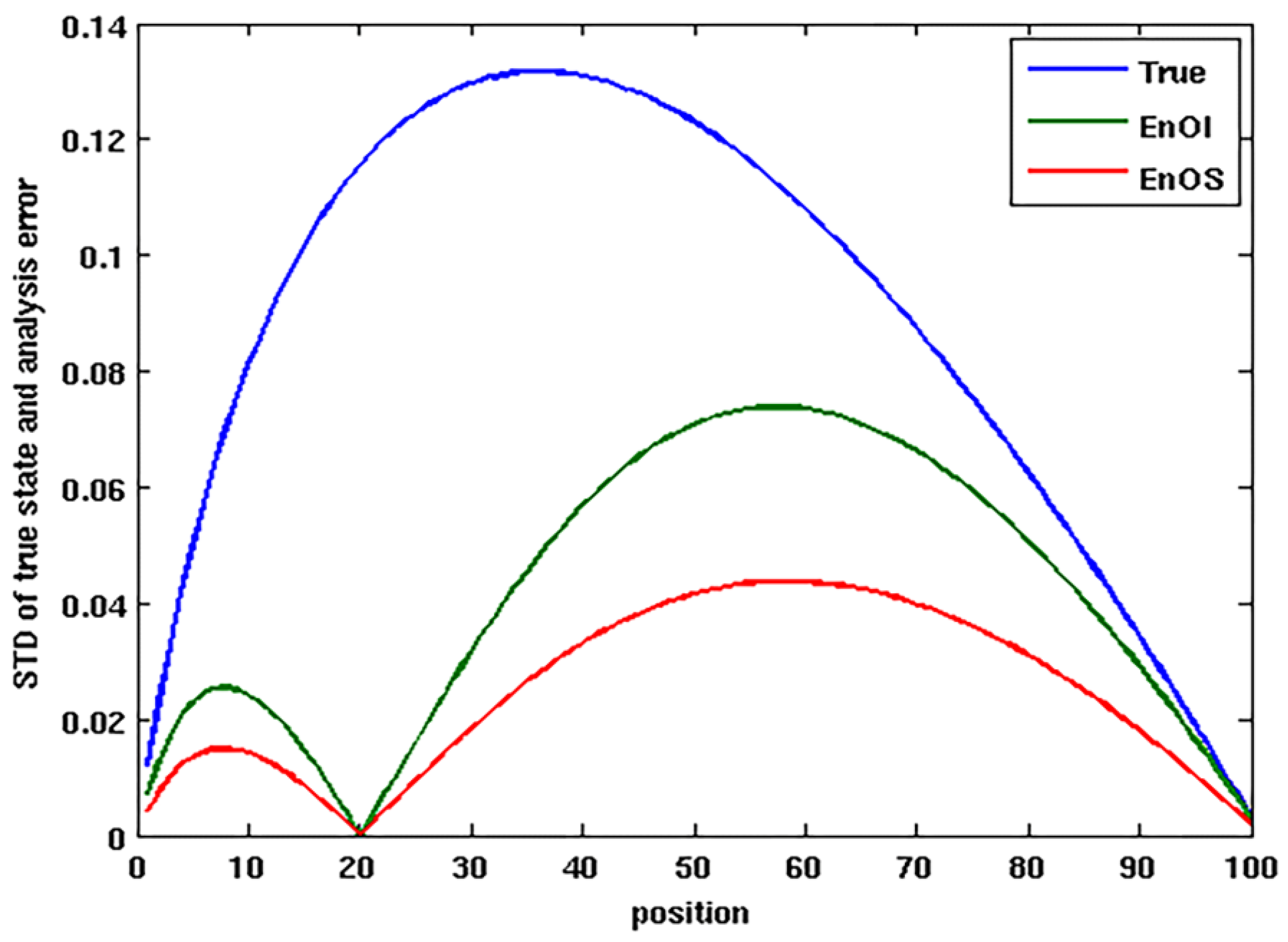
3. Idealized Linear Ocean Model

We now introduce a highly idealized, linear barotropic ocean model in order to illustrate the performance of the smoother scheme. One advantage of using such a simple model is the possibility of obtaining the theoretical Kalman gain of EnOS and the corresponding analytical skill of the assimilating scheme.

The idealized ocean model has a rigid lid and a flat bottom and lies on a mid-latitude $\beta$-plane. Its stream function $\psi$ evolves according to the following forced Rossby wave equation [31]:

$$\frac{\partial }{\partial t}\left(\frac{{\partial }^2\psi }{\partial x^2}\right)+\frac{\partial \psi }{\partial x}=-\delta \frac{{\partial }^2\psi }{\partial x^2}+F$$

(17)

where $x$ is the east–west coordinate that is non-dimensionalized by the ocean width $L$ and $t$ is time that is non-dimensionalized by ${\left(L\beta \right)}^{-1}$, which is on the order of 1 day for a typical mid-latitude basin. The parameter $\delta$ is the width of the western boundary currents region $L$; its reciprocal is the spin-down time of the system in non-dimensional time. $F$ denotes forcing by the wind stress curl and is allowed to vary with both $x$ and $t$; its characteristic magnitude sets the scale for $\psi$. The coastal boundary conditions are $\psi =0$ along the west $\left(x=0\right)$ and east $\left(x=1\right)$ boundaries of the model domain. The spatial domain was divided into 100 grids in this study. The time step was set to 1 day, and the initial condition was set to 0 at all grids.

In Figure 1, the “reference” or “true” field shows the stream function corresponding to a random forcing, which it represents in terms of westward propagating barotropic Rossby waves. In the western boundary currents region, the Rossby waves were dissipated after reflecting as slowly moving, short Rossby waves. Corresponding to the close boundary condition at the east and west boundaries, the variances in the stream function at both boundaries was 0 and reached its maximum value at the eastern part of the region near the middle.

We assumed there was only one observation located at $\left(x=0.2\right)$, which was available at every time step. The first guess or “forecast” field was produced from the same model but with no forcing. As expected, there was no any signal in the forecast field. We then used the assimilation methods (EnOI and EnOS) to illustrate how the “true” field could be recovered from the limited observation. In this experiment, the observations were taken from the “truth” run and were error-free. Therefore, the matrixes of observation error were set to 0 in the two assimilation schemes. The background error covariance matrixes were estimated from a 3-year training run. In the EnOS system, the assimilation window was set to two days (two time steps included) and the time lag was one day.

The analysis states from EnOI and EnOS are shown in the right two panels in Figure 1. The analysis field of EnOI was generally good and the entire pattern of the stream function matched with the reference, but the amplitude of the analyzed stream function was overestimated on the west side and underestimated on the east side. The reason for these unreal analysis features was due to the background error covariance not being “flow dependent”. When the background error covariance was critically calculated from linear Kalman filter, the analysis field was much closer to the “true” field (not shown). The analysis field for EnOS was much better than the analysis field of EnOI, although the unreal features also appeared in the EnOS. It is sensible that the analysis field was more energetic on the west side of observation because the Rossby waves were propagating westward, therefore the variation introduced by assimilation was concentrated into this region. The overperformance of EnOS was especially significant in the region east of the observation, where there was almost no signal in the EnOI analysis, while EnOS successfully extended information to this region from the observations.

As shown in Figure 2, the RMSEs of both approaches were smaller than the STD of the “true” field, which indicated that both methods were effective in reducing model errors. At the observation position $\left(x=0.2\right)$, the RMSE was close to 0 for both methods because the observation was error-free. The error grew gradually along with the increment in distance from the observation. The EnOS scheme was more efficient and effective in expanding the observation information to the model domain. As expected, the error of EnOS analysis was significantly less than that of EnOI in the whole domain. The advantage was even more pronounced when the observations were located near the boundary, where the EnOI method did not perform well.

4. Sensitivity Analysis of Time-Dependent Term

4.1. Data

In Section 3, we demonstrated the effectiveness of the two methods in correcting for model errors using an approximate, ideal ocean model. To further validate the performance of the two methods using real data, we conducted twin experiments using the reanalysis dataset. Data for the ocean assimilation experiments were obtained from the 1/12° daily average reanalysis dataset in GLORYS12v1 ocean reanalysis version GLOBAL_REANALYSIS_PHY_001_030, which is available online at: https://marine.copernicus.eu (accessed on 7 March 2022) [32]. This dataset performs well relative to the 2013 World Ocean Atlas climatology and in situ data (global mean in situ temperature error below 0.1 °C). Across the in-analysis dataset, the regional error is less than 0.4 °C and the global mean sea surface temperature is close to the observed value, with a mean error of less than 0.1 °C [33]. The global positive SST linear trend is highly consistent with the AVHRR data, thus the sea surface temperature in this dataset was chosen as the state variable for our assimilation experiments.

As a prototype algorithm, we only used the above reanalysis data for the EnOI and EnOS data assimilation twin experiments without model integration based on the analysis field, and did not discuss the effect of assimilation on the model integration process, but only the effect of assimilation on the current moment. We used the coastal waters of China and adjacent seas as the target study region, specifically in the range (15° N–30° N, 105° E–130° E). The EnOI experiment was set up with the reanalysis SST from 5 January 2007–4 January 2017 as the “true field” or “target field”. In order to construct a “background field” with errors, the reanalysis data of the year before the corresponding date of the “true field” was used as the “background field” [34]. The “background field” errors were formed by the difference in the reanalysis SST between two years. The experimental setup of EnOS was based on EnOI with one additional historical moment of observation for each assimilation; the time interval between two assimilation moments was set to 1 day. The dataset of 31 December 2013–31 December 2014 was used to construct 365 samples for the background field and of 1 January 2015–31 December 2015 for the target field. Points were selected from the corresponding target fields without perturbing the observations, so the observation error covariance was set to 0.

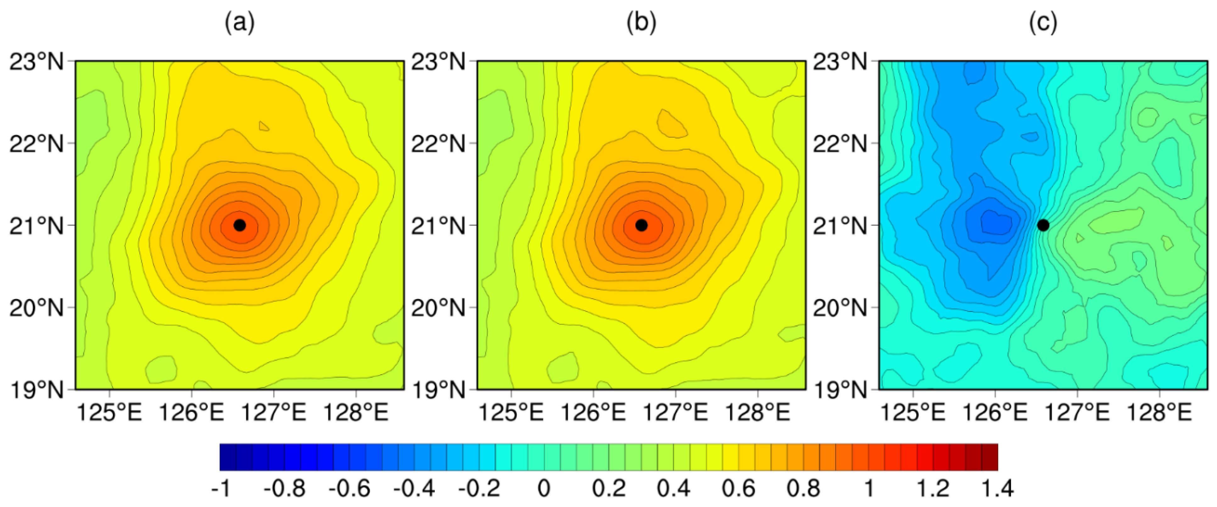
4.2. Single-Point Observation Experiments

In this section, we describe the design of three groups of single-point observation options (A, B, and C). As shown in Figure 3, we selected three representative regions with their own characteristics [35]:

The group A single-point observation experiment was located near the Kuroshio mainstream in the East China Sea. The Kuroshio mainstream flows from west to east and the flow velocity becomes faster in spring and winter, making the temperature gradient on both sides of the mainstream larger, and there is an obvious nuclear fluid structure [36]. The group B single-point observation experiment was located in the northern margin of the South China Sea. The region is sometimes dominated by circulation and sometimes there is a strong vortex, and the eddy current interaction signals are complex. The circulation structure in the northern margin of the South China Sea is relatively weak and slightly chaotic, with high surface temperatures and slight seasonal fluctuations throughout the year [37,38]. The group C single-point observation experiment was located in the region of subtropical countercurrent in the western North Pacific with large eddy kinetic energy, which was more concentrated near 20° N–22° N. There are a huge number of mesoscale eddies in the region; the active eddies have obvious westward propagation characteristics, their temperature-distribution characteristics are mainly influenced by the latitude position, and the temperature changes are consistent with the frequent eddy activity [23].

The spatial distribution characteristics and time variation of SST in the above three regions were obviously different, so these three regions were selected for experiments in this study to verify the universality of the time-dependent term of EnOS in different situations. In the range of plus or minus 2° from the observation point, we performed a sensitivity analysis on the observed features extracted from the three groups of experiments separately and discussed the effect of time lag on the Kalman filter.

Figure 4a shows that the Kuroshio mainstream in the background field was located southward and deviated from the observation point, and there was a clear distribution of eddies on both sides with a wide flow amplitude and high temperature. As shown in Figure 4b, the Kuroshio Current in the target field showed a southwest–northeast trend; the observation point was in the center of the Kuroshio mainstream. The SST of the mainstream was obviously higher than that of the two sides and the temperature gradually decreased to the north, with a significant decrease near 28.5° N. There were no small-scale eddies formed on either side of the Kuroshio Current on that day due to coiling.

Within ±2° of the observation point, the RMSE was 0.52 °C for the EnOI scheme and 0.49 °C for the EnOS scheme, a decrease of about 5.8% relative to EnOI. Combined with Figure 4c,d, it can be seen that overall, both seemed to have improved, but the improvement was not obvious. Comparatively speaking, EnOS was a bit better, as the cooling of the northern end of the Kuroshio Current in Figure 4d was more obvious and the intensity of the small-scale eddies on both sides had weakened, reflecting the advantage of EnOS in improving the details.

The distribution of isotherms showed that the overall temperature of the analysis field of EnOI was high, especially in the southwest direction of the observation point, which had a significant warm bias, while EnOS eliminated the warm bias in this direction to a certain extent and had a better correction effect. The overall temperature of the analysis field of EnOS was lower than that of EnOI and the temperature gradient on both sides of the Kuroshio mainstream was larger. Although the target field was not reached, EnOS had a better performance in many regions; for example, the warm bias around the observation point and the intensity of small-scale eddies were improved and the temperature gradient of the target field was approximately recovered in the mainstream region northeast of the observation point.

Neither method had a significant correction effect, suggesting that a single point provide too little information to improve details. Although EnOS performed better with additional historical data, it was still not enough to produce a significant effect.

To illustrate more intuitively the range and strength of the improvement of EnOS over EnOI, we rewrote Equations (11) and (13) to obtain Equations (18) and (19), where $X_a$ represents the analysis field at the moment $t$, $X_b$ represents the background field at the moment $t$, and the product term represents the analysis increment.

$$X_a=X_b+\left(\begin{array}{cc}{K}_{t,t}& K_{t,t_{-1}}\\ K_{t-1,t}& K_{t-1,t-1}\end{array}\right)\left(\begin{array}{c}\mathsf{\Delta }{Y}_t\\ \mathsf{\Delta }{Y}_{t-1}\end{array}\right)$$

(18)

$$\mathsf{\Delta }{X}_a=K_{t,t}\mathsf{\Delta }{Y}_t+K_{t,t-1}\mathsf{\Delta }{Y}_{t-1}$$

(19)

Adding the time-dependent term $K_{t,t-1}\mathsf{\Delta }{Y}_t$ to the right-hand side of Equation (19) and rearranging gives:

$$\mathsf{\Delta }{X}_a=\left(K_{t,t}+K_{t,t-1}\right)\mathsf{\Delta }{Y}_t-K_{t,t-1}\left(\mathsf{\Delta }{Y}_t-\mathsf{\Delta }{Y}_{t-1}\right)$$

(20)

The first term on the right-hand side of the medium sign in Equation (20) represents the analysis increment generated by the observation increment at the current moment in EnOS, which is equivalent to the analysis increment at moment $t$ in EnOI, and the second term represents the additional information brought by the historical observation in EnOS. We let $K_0=K_{t,t}+K_{t,t-1}$, $K_1=K_{t,t-1}$, $\mathsf{\Delta }Y=\mathsf{\Delta }{Y}_{t-1}-\mathsf{\Delta }{Y}_t$. Analogous to the linear advection equation that is obtained in Equation (20), the variation in the observed increment in time corresponds to $\mathsf{\Delta }Y$, $K_1$ projects it from time to space, and the additional term obtained by multiplying the two corresponds to the direction and form of the increment propagating in space.

As shown in Figure 5a,b, since the first term of EnOS could achieve a correction comparable to EnOI, as we expected, the analytical gains of the two schemes were very similar for $t$ moments. In the analysis of Figure 4, it was clear that EnOS was closer to the target field throughout the Kuroshio mainstream, which was consistent with the characteristics shown in Figure 5c. The negative Kalman gain near the entire region acted on $\mathsf{\Delta }Y$, and the additional term made the overall temperature of the analytical field of EnOS lower than that of EnOI, and performed better particularly in the correction of the mainstream and the eddies on both sides.

In Figure 5c, $K_1$ is positive in the southwest side of the observation point, and negative in all other directions, indicating that the observation increment in the observation point of group A was propagated from southwest to northeast with the observation point as the center, which was consistent with the actual Kuroshio Current. Since the advantage of EnOS was obtained by $K_1$ acting on $\mathsf{\Delta }Y$, by analyzing the analysis field of both schemes on 1 January 2015, we found that the value of $\mathsf{\Delta }Y$ in the additional term of EnOS was 0.22 °C and the range of values of the additional term obtained under the action of $K_1$ was −0.044 °C to 0.198 °C. Combined with Figure 5, it can be seen that the positive effect of the additional term at the observation point was manifested in the propagation of the fluctuation signal from southwest to northeast. The experiments in group A showed that the addition of additional terms could effectively capture the fluctuation signal at the observation point, allowing the EnOS scheme to obtain more effective information and to correctly map the time-propagated signal in the region to space.

We continued to analyze the other two experiments; the results showed that EnOS performed better than EnOI. In Figure 6 and Figure 7a,b, it can be seen that the results of the two groups of experiments in B and C were the same as those in group A and the Kalman gain was similar to $K_0$ in terms of morphology and intensity, so we analyzed the advantage of EnOS using $K_1$. The EnOS scheme was calculated to have a 3.2% decrease in the RMSE relative to EnOI, which was a small but positive improvement. As can be seen in Figure 6c, the weak intensity of the gain $K_1$ indicated that the propagation signal of the background error was weaker at the observation point in the northern margin of South China Sea, but the left-high–right-low distribution presented by $K_1$ reflected the propagation characteristics and the propagation direction from east to west at this point. The additional term of the group B experiment was minor compared with group A because the fluctuation signal in the northern margin of South China Sea was complex and weak at the observation point and there was no obvious pattern of propagation characteristics in this region compared with the group A and C experiments. The above results showed that the additional term performed differently for different regions; further research is needed to better utilize its capabilities.

The observation point of group C was near the 21° N longitude line in the western North Pacific, which is located in the subtropical countercurrent zone with frequent eddy activities and obvious westward propagation characteristics. The results for the experiment in group C were better than those for group B. The assimilation effect of EnOS was improved by 4.9%. According to Figure 6c and Figure 7c, the difference between the two groups of experiments was the difference in the strength of the fluctuation signal at the observation point, thus we concluded that the stronger the fluctuation signal, the more obvious the additional term advantage. Figure 7c shows that $K_1$ had obvious intensity changes on the east and west sides of the observation point; the fluctuation signal propagated from east to southwest, which was consistent with the actual situation. In addition, as can be seen in Figure 6a,b, similar to Figure 6, the Kalman gain approximations of the two experiments had obvious isotropic propagation patterns but $K_1$ differed more in intensity and morphology, showing different characteristics of different regions. In other words, due to the lack of time-varying new information, the analysis increments obtained by the EnOI scheme corrected only for the current moment could not characterize the motion pattern of the seawater at the observation point.

The three groups of experiments corresponded to different regions with different characteristics. In the experimental results, all three groups had positive effects, indicating that the inclusion of additional terms was necessary. The most significant effect was observed in the East China Sea Kuroshio experiments in group A, followed by the group C experiments located in the subtropical countercurrent zone, while the group B experiment in the northern margin of South China Sea had the least enhancement. Combined with Figure 5c, Figure 6c and Figure 7c, the above results were analyzed corresponding to the characteristics of different sea areas. The group A experiment was located in the Kuroshio mainstream with a large temperature gradient, fast propagation characteristics of seawater flow, and the largest fluctuation signal intensity. The second was group C, where the abundant mesoscale eddies had obvious westward propagation characteristics, while the signal propagation strength was the weakest at the observation point for group B. We found that the error propagation capability was consistent with its own temperature propagation signal, and thus the advantage of the additional term was more pronounced in the region where the temperature propagation was stronger.

In general, the EnOS scheme adds a mapping of the incremental historical observation at moment $t$ for moment $t-1$ and can also improve the analysis results of the current moment. One term of EnOS relative to the addition of EnOI reflects the linear law of the spatial propagation of the background field error, so the spatial distribution of the state of the increment in the analysis is not only related to the change of the background field error at two moments, but it also will change with time with a certain “flow dependent” character. The additional term was able to represent the distribution and propagation characteristics of the model error in different regions, which was closely related to the signal propagation strength at the observation point and could represent regional differences without special treatment.

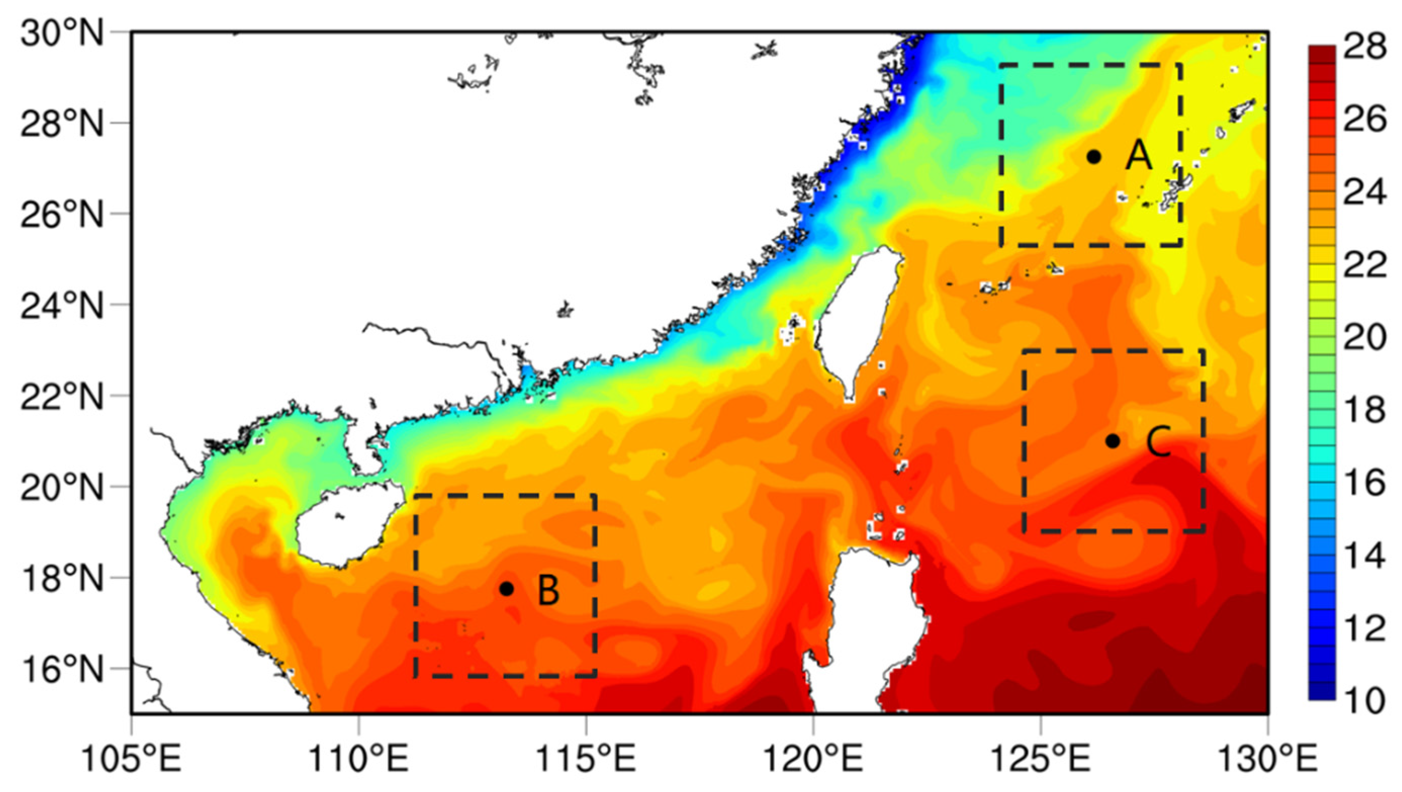
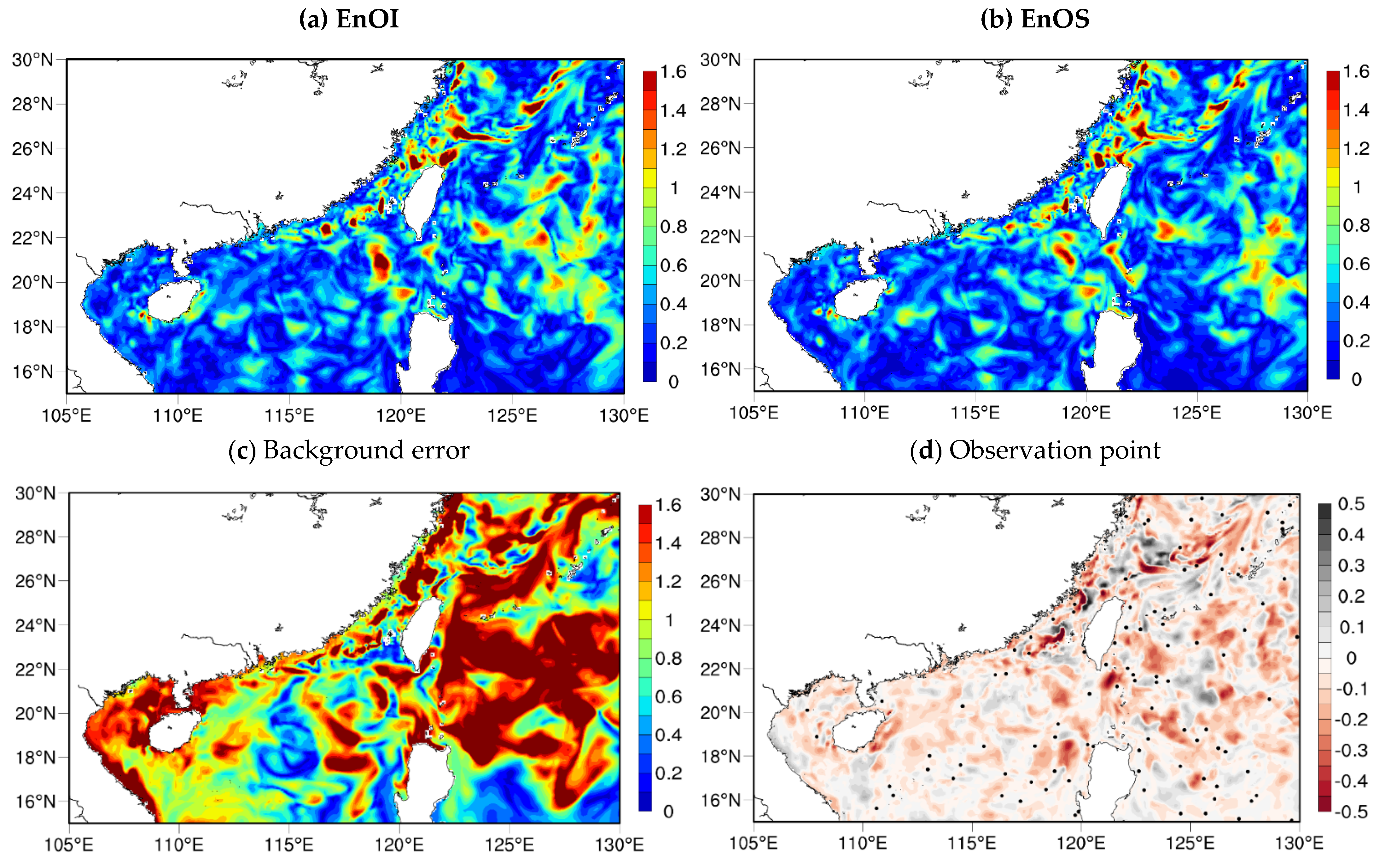
5. Validation Using the Reanalysis Data

Due to the limited improvement of the single-point observation data detailed in Section 4, we examined the effect of EnOS by increasing the number of observation points. We illustrated the performance of EnOI and EnOS using the same dataset described in Section 4.1 with a twin test of multiple observation points in the target region [39]. The background field, target field, and observation data used in the experiment were obtained from the above reanalysis data. The background field and other settings were the same as those of the single-point observation experiments except that the number of observation points was increased to 100. Among them, the observation points were a randomly selected 100 points in the target research region (15° N–30° N, 105° E–130° E); the SST data of the corresponding position in the target field was used as the observation value. In this part of the study, we performed assimilation for the entire year of 2015 using EnOI and EnOS and specifically analyzed the assimilation effect caused by adding historical observations under the interaction of multiple observations.

Both schemes improved the error of the background field well in Figure 8a,b: the RMSE dropped to near 0.2 °C in most of the regions. Although EnOI had a weak advantage in the nearshore and some other regions, EnOS performed much better than EnOI in the entire target study region. For example, the RMSE of EnOS was significantly reduced or even disappeared in the East China Sea Kuroshio, on both sides of Luzon Strait, etc. The RMSE of a large region in the western North Pacific near Taiwan decreased by about 0.3 °C relative to EnOI. The advantage of the EnOS scheme was more obvious with the increased number of observation points. The error distribution of the background field and the target field in the two twin experiments for the entire year is shown in Figure 8c. The error of the background field was large, especially in the Kuroshio Current, the western North Pacific, and the Beibu Gulf.

We used the spatial distribution obtained by subtracting the RMSE of EnOI and EnOS throughout the year as the background; the black dots in Figure 8d are the 100 observation points. Most of the two methods were white at the location where the observation point was centered, implying that there was approximately the same RMSE at that point. This was because the observation data were not perturbed in this experiment and the observation error was set to 0. Both sets of experiments could fully obtain the true field information at the observation point.

For the purpose of this analysis, we continued to count the performance of the time-averaged RMSE for EnOI and EnOS over the four quarters. Combined with

Table 1. RMSEs of EnOI and EnOS in four seasons.

Evaluation Criteria	Method	Winter	Spring	Summer	Autumn
Root-Mean-Square error (RMSE)	EnOI	0.54	0.58	0.41	0.40
	EnOS	0.48	0.54	0.39	0.38
	Performance gain	11.02%	7.15%	3.03%	2.35%

, it can be seen that the best performance was in the spring and winter seasons with a correction intensity of about 11% and 7%, followed by about 3% in summer, and with the least significant performance of only 2% in autumn.

The performance of the two schemes in different regions in two typical seasons can be clearly seen in Figure 9. Despite the better performance of EnOI in some regions, the overall dominance of EnOS was obvious in both seasons (the distribution of red is larger than black), especially in winter. The darker color in winter in the figure indicates that the respective advantages of the two schemes were more prominent in winter, especially in the East China Sea Kuroshio. This was due to the strong temperature gradient of the seawater on both sides of the Kuroshio mainstream in the spring and winter seasons, as well as the fluctuation signal being harder to capture, thus the correction difference reached ±0.5 °C for each of the two schemes in this region. In addition, unlike the obvious nuclear fluid structure in winter, the sea surface temperature receded significantly in autumn and the path of the Kuroshio Current is not obvious; the two schemes performed comparably with a relative advantage of only about ±0.2 °C [19]. Although different seasonal features led to different assimilation effects, the better performance of EnOS in the East China Sea Kuroshio was sufficient to show that the addition of temporal correlation allowed it to capture more detailed signals. At the same time, more information superposition also may have led to spurious correlations, making EnOS perform worse than EnOI in some regions.

In similar situations in other regions, there were obvious seasonal characteristics in winter; the EnOS scheme had obvious advantages in the Kuroshio mainstream, the Beibu Gulf, and the western North Pacific, while the advantages were not obvious in autumn, and both schemes had advantages and disadvantages in most regions. In summary, the difference in performance between the two schemes in different seasons was clear, therefore the 21° N latitude band (black dashed line in Figure 9) was chosen to analyze the fluctuating signal over time and further discuss why the seasonal differences existed.

As shown in Figure 10a, the fluctuation signal of the target field showed a trend toward a low temperature in winter and spring and a high temperature in summer and autumn with time. We found that with the increase in time, the seawater in the northern margin of South China Sea had obvious propagation characteristics in winter and spring, while the fluctuating signal was smoother and mostly low-frequency after 150 days in summer and autumn. There was a clear westward propagation process in the western North Pacific of the Luzon Strait (120° E); the figure shows a predominantly high-frequency signal that indicated frequent eddy activity, which was consistent with the actual situation.

In Figure 10, it is clear that the analysis fields of both schemes were similar to the target field in terms of the fluctuation signal patterns and sea surface temperature distributions, indicating that both analysis fields performed better in terms of the correction effect. However, the correction of EnOS for the high-frequency signal provided more details and had a very great advantage.

We found that many small-scale fluctuations in the western North Pacific in winter and spring that propagated westward did not appear in the analysis field of EnOI, while their intensity and velocity in EnOS were very close to those of the target field (True). An example is the performance of EnOS during the first 100 days of winter, which had a spatial signal extension near the target field in both the east and west directions, especially in the region of subtropical countercurrent in the western North Pacific. However, the advantage of EnOS was not obvious in the autumn of days 240–310 due to the absence of significant propagation characteristics. Summer performed better, with EnOS reproducing two low-temperature regions of the target field at 112° E on day 210 and 117° E on day 240, while EnOI reproduced only 1/2 of the total region and smoothed out the high-frequency signal between the two lines of longitude.

Since there were no obvious propagation characteristics in the northern margin of the South China Sea in summer and autumn, a combination with Figure 9 showed that the two scenarios performed comparably. In addition, east of the Luzon Strait, especially around 124° E–128° E and 110° E, EnOS successfully portrayed the detailed east–west fluctuation signal of the target field relative to EnOI. According to the analysis in Section 4, the stronger the fluctuating signal, the greater the weight of the additional gain in the region where the propagation characteristics were obvious. Thus, EnOS showed a clear advantage in the entire region in winter and spring, as well as in the western North Pacific in summer and autumn, as shown in Figure 9 and Figure 10. It was also demonstrated that the advantage of EnOS in capturing such detailed fluctuating signals was due to its ability to capture the error-propagation signal, which arose from the second term in Equation (20). We next performed sample space averaging in order to evaluate the two schemes more intuitively.

As shown in Figure 11, the 365 samples were averaged over the spatial grid points to obtain the RMSE performance for each day of the year. The yearly average RMSE was 0.48 for EnOI and 0.45 for EnOS. The RMSE decreased by 6.4%, indicating that EnOS had a better correction effect throughout the year. The RMSE was significantly lower in winter and spring and did not tend to diminish over time, while in summer and autumn, both protocols had a lower RMSE, thus diminishing the improvement effect of EnOS.

Table 1 shows the performance of the two schemes in each of the four seasons. We found that best performance in winter, with EnOS reducing the RMSE by 11.02%. Spring followed, although its original RMSE was the largest, with a correction effect of 7.15%. Although the RMSE decreased to about 0.4 °C in summer and autumn, which was a good improvement for both methods, EnOS still had an advantage of about 3%. In short, in line with the previous analysis, EnOS outperformed EnOI throughout the year.

Overall, the improvement in the correction power of EnOS relative to EnOI with multiple observations averaged about 6% throughout the year and nearly 10% in winter and autumn, a very significant improvement. The multi-point observations experiment illustrated that more effective information enabled the additional term to more reasonably characterize the spatial signal. At the same time, in places where the fluctuation signal was strong throughout the target region, the additional term not only represented the direction and intensity of the fluctuation, but also captured the high-frequency signal that more closely resembled the target field, consistent with the conclusions given in Section 4.

6. Discussion and Conclusions

We developed a new ensemble assimilation algorithm called EnOS that was straightforward extended from the EnOI scheme. Compared to EnOI, the main advantage of EnOS was that it was capable of benefiting the estimate of the present state from the time history of the observations. Although the background error distribution did not change with time, this frame was designed to represent the variation in interesting frequencies by employing the cross-covariance of background fields between each time step. This made EnOS able to constraint the propagation features of certain waves and spread observation information to the model grids more reasonably.

EnOS was evaluated using a one-dimensional linear ocean model. The comparisons between EnOS and traditional EnOI showed that the new approach was more efficient and effective in reducing model errors, especially in the region far away from the observations. Then, single-point observation experiments were conducted in regions with different fluctuation characteristics, such as the East China Sea Kuroshio, the northern margin of South China Sea, and the western North Pacific. After evaluation using three sets of experiments, we found that EnOS was better than EnOI for all three groups and that the additional terms had positive effects of different strengths for different regions. The regions of the two experimental groups A and C had obvious spatial propagation characteristics, while the good performance of EnOS indicated that additional terms with “flow dependent” characteristics in EnOS were necessary. The experiments in group B still had the advantage of EnOS despite the current region without obvious spatial propagation characteristics, indicating that the additional term was still effective in capturing and exploiting the spatial signal when the fluctuation signal was weak. In general, the stronger the fluctuation signal in the target region, the more obvious the advantage of the additional term.

In addition, we used the reanalysis dataset to perform twin tests of multiple observation points in the target study region. The results showed that EnOS performed better throughout the year, with a 6.4% decrease in the RMSE relative to EnOI. Further analysis showed that the winter and spring corrections were highly effective, with the RMSE decreasing by 11.02% and 7.15% for the two scenarios, respectively. Through experimental validation, we found that the addition of a time-dependent term allowed EnOS to recover more small scales than EnOI, such as some eddies that were not detected by the observations. This was a very useful capability to fill the gap between observations.

Although the results with ideal models were encouraging, this approach still had some defects in practice. As we noticed in the experiments, the performance of this method was affected by selection of time lags. To demonstrate the smoothing effect of temporal correlation, the experiments in this paper all chose a fixed time lag, thus affecting the EnOS performance for current regions with different characteristics. For some areas, the assimilation run with EnOS did not show a significant improvement. This was reasonable because the cross-covariance between two time steps may not provide much useful information if the time lags are selected improperly. Another noticeable issue of this approach was that it did not always perform better than EnOI. The reason might lie in the fact that there were more than one regime in the experiment period, so the derivative information could not supply much useful information in some regimes. This issue still remains to be solved in a future study. In summary, the new scheme with “flow dependent” properties remained computationally simple and efficient. Through the smoothing effect of historical moments, EnOS obtained a stronger ability to capture scale features, which is promising for future operational ocean assimilation systems.

The present study was a necessary step in developing a practical assimilation system for a relocatable ocean model that can be applied on a shelf. Our next step is to implement this new algorithm in realistic ocean models to improve ocean current simulation capabilities. Due to the complex current field near shelves, where tides and baroclinic currents are both important, adaptive time lag selection in different seas according to the complex signals of fluctuations will be greatly challenging.

References

1. Burgers, G.; Leeuwen, P.J.; Evensen, G. Analysis scheme in the Ensemble Kalman Filter. Mon. Weather Rev. 1998, 126, 1719–1724. [Google Scholar] [CrossRef]
2. Evensen, G.; Van Leeuwen, P.J. Assimilation of gestat altimeter data for the Agulhas current using the ensemble Kalman filter. Mon. Weather Rev. 1996, 124, 85–96. [Google Scholar] [CrossRef]
3. Oke, P.R.; Chamberlain, M.A.; Fiedler, R.A.S.; de Oliveira, H.B.; Beggs, H.M.; Brassington, G.B. Combining Argo and Satellite Data Using Model-Derived Covariances: Blue Maps. Front. Earth Sci. 2021, 9, 696985. [Google Scholar] [CrossRef]
4. Wikle, C.K.; Berliner, L.M. A Bayesian tutorial for data assimilation. Phys. D Nonlinear Phenom. 2007, 230, 1–16. [Google Scholar] [CrossRef]
5. Gordon, N.; Salmond, D.; Smith, A. Novel approach to nonlinear/non-Gaussian Bayesian state estimation. IEE Proc. F (Radar Signal Process.) 1993, 140, 107–113. [Google Scholar] [CrossRef]
6. Evensen, G. Sequential data assimilation with a nonlinear quasi-geostrophic model using Monte Carlo methods to forecast error statistics. J. Geophys. Res. Oceans 1994, 99, 10143–10162. [Google Scholar] [CrossRef]
7. Houtekamer, P.L. The Construction of Optimal Perturbations. Mon. Weather Rev. 1995, 123, 2888–2898. [Google Scholar] [CrossRef]
8. Keppenne, C.L. Data assimilation into a primitive-equation model with a parallel ensemble Kalman filter. Mon. Weather Rev. 2000, 128, 1971–1981. [Google Scholar] [CrossRef]
9. Mitchell, H.L.; Houtekamer, P.L.; Pellerin, G. Ensemble Size and Model-Error Representation in an Ensemble Kalman Filter. Mon. Weather Rev. 2002, 130, 2791–2808. [Google Scholar] [CrossRef]
10. Mignac, D.; Tanajura, C.A.S.; Santana, A.N.; Lima, L.N.; Xie, J. Argo data assimilation into HYCOM with an EnOI method in the Atlantic Ocean. Ocean Sci. 2015, 11, 195–213. [Google Scholar] [CrossRef] [Green Version]
11. Evensen, G. The Ensemble Kalman Filter: Theoretical formulation and practical implementation. Ocean Dyn. 2003, 53, 343–367. [Google Scholar] [CrossRef]
12. Oke, P.R.; Allen, J.S.; Miller, R.N.; Egbert, G.D.; Kosro, P.M. Assimilation of surface velocity data into a primitive equation coastal ocean model. J. Geophys. Res. Oceans 2002, 107, 5-1–5-25. [Google Scholar] [CrossRef]
13. Oke, P.R.; Schiller, A.; Griffin, D.A.; Brassington, G.B. Ensemble data assimilation for an eddy-resolving ocean model of the Australian region. Q. J. R. Meteorol. Soc. 2005, 131, 3301–3311. [Google Scholar] [CrossRef]
14. Belyaev, K.; Kuleshov, A.; Smirnov, I.; Tanajura, C.A.S. Generalized Kalman Filter and Ensemble Optimal Interpolation, Their Comparison and Application to the Hybrid Coordinate Ocean Model. Mathematics 2021, 9, 2371. [Google Scholar] [CrossRef]
15. Oke, P.R.; Sakov, P.; Corney, S.P. Impacts of localisation in the EnKF and EnOI: Experiments with a small model. Ocean Dyn. 2006, 57, 32–45. [Google Scholar] [CrossRef]
16. Wang, X.; Hamill, T.M.; Whitaker, J.S.; Bishop, C.H. A Comparison of Hybrid Ensemble Transform Kalman Filter–Optimum Interpolation and Ensemble Square Root Filter Analysis Schemes. Mon. Weather Rev. 2007, 135, 1055–1076. [Google Scholar] [CrossRef]
17. Wan, L.; Bertino, L.; Zhu, J. Assimilating Altimetry Data into a HYCOM Model of the Pacific: Ensemble Optimal Interpolation versus Ensemble Kalman Filter. J. Atmos. Ocean. Technol. 2010, 27, 753–765. [Google Scholar] [CrossRef]
18. Zhang, S.; Anderson, J.L. Impact of spatially and temporally varying estimates of error covariance on assimilation in a simple atmospheric model. Tellus A Dyn. Meteorol. Oceanogr. 2016, 55, 126–147. [Google Scholar] [CrossRef]
19. Barth, A.; Weisberg, R.H.; Alvera-Azcárate, A. Assimilation of high-frequency radar currents in a nested model of the West Florida Shelf. J. Geophys. Res. Oceans 2008, 113. [Google Scholar] [CrossRef]
20. Xu, J.; Huang, J.; Gao, S.; Cao, Y. Assimilation of high frequency radar data into a shelf see circulation model. J. Ocean Univ. China 2014, 13, 572–578. [Google Scholar] [CrossRef]
21. Castruccio, F.S.; Karspeck, A.R.; Danabasoglu, G.; Hendricks, J.; Hoar, T.; Collins, N.; Anderson, J.L. An EnOI-Based Data Assimilation System With DART for a High-Resolution Version of the CESM2 Ocean Component. J. Adv. Model. Earth Syst. 2020, 12, e2020MS002176. [Google Scholar] [CrossRef]
22. Scott, K.A.; Chen, C.; Myers, P.G. Assimilation of Argo Temperature and Salinity Profiles Using a Bias-Aware EnOI Scheme for the Labrador Sea. J. Atmos. Ocean. Technol. 2018, 35, 1819–1834. [Google Scholar] [CrossRef]
23. He, Z.; Thompson, K.R.; Ritchie, H.; Lu, Y.; Dupont, F. Reducing Drift and Bias of a Global Ocean Model by Frequency-Dependent Nudging. Atmosphere-Ocean 2014, 52, 242–255. [Google Scholar] [CrossRef]
24. Katavouta, A.; Thompson, K.R. Downscaling ocean conditions: Experiments with a quasi-geostrophic model. Ocean Model. 2013, 72, 231–241. [Google Scholar] [CrossRef]
25. McCalpin, J.D.; Haidvogel, D.B. Phenomenology of the low-frequency variability in a reduced-gravity, quasi-geostrophic double-gyre model. J. Phys. Oceanogr. 1996, 26, 739–752. [Google Scholar] [CrossRef]
26. Liu, C.; Zhang, S.; Li, S.; Liu, Z. Impact of the time scale of model sensitivity response on coupled model parameter estimation. Adv. Atmos. Sci. 2017, 34, 1346–1357. [Google Scholar] [CrossRef]
27. Cohn, S.E.; Sivakumaran, N.S.; Todling, R. A Fixed-Lag Kalman Smoother for Retrospective Data Assimilation. Mon. Weather Rev. 1994, 122, 2838–2867. [Google Scholar] [CrossRef]
28. Li, H.; Kalnay, E.; Miyoshi, T. Simultaneous estimation of covariance inflation and observation errors within an ensemble Kalman filter. Q. J. R. Meteorol. Soc. 2009, 135, 523–533. [Google Scholar] [CrossRef]
29. Miyoshi, T.; Kalnay, E.; Li, H. Estimating and including observation-error correlations in data assimilation. Inverse Probl. Sci. Eng. 2012, 21, 387–398. [Google Scholar] [CrossRef]
30. Anderson, J.L.; Anderson, S.L. A monte Carlo implementation of the nonlinear filtering problem to produce ensemble assimilations and forecasts. Mon. Weather Rev. 1999, 127, 2741–2758. [Google Scholar] [CrossRef]
31. Gill, A.E. Atmosphere-Ocean Dynamics; Academic Press: San Diego, CA, USA, 1982; pp. 507–513. [Google Scholar]
32. Jean-Michel, L.; Eric, G.; Romain, B.-B.; Gilles, G.; Angélique, M.; Marie, D.; Clément, B.; Mathieu, H.; Olivier, L.G.; Charly, R.; et al. The Copernicus Global 1/12° Oceanic and Sea Ice GLORYS12 Reanalysis. Front. Earth Sci. 2021, 9, 698876. [Google Scholar] [CrossRef]
33. Drévillion, M.; Régnie, C.; Lellouche, J.; Garris, G.; Bricaud, C.; Hernandez, O. Quality Information Document for Global Ocean Reanalysis Products GLOBAL-REANALYSIS-PHY-001-030; Copernicus, Marine Environment Monitoring Service: Ramonville-Saint-Agne, France, 2021; pp. 1–48. [Google Scholar]
34. Wu, B.; Zhou, T.; Zheng, F. EnOI-IAU Initialization Scheme Designed for Decadal Climate Prediction System IAP-DecPreS. J. Adv. Model. Earth Syst. 2018, 10, 342–356. [Google Scholar] [CrossRef]
35. He, B.; Mitchell, H.L.; Charette, C.; Houtekamer, P.L.; Buehner, M. Intercomparison of Variational Data Assimilation and the Ensemble Kalman Filter for Global Deterministic NWP. Part I: Description and Single-Observation Experiments. Mon. Weather Rev. 2010, 138, 1550–1566. [Google Scholar] [CrossRef]
36. Ichikawa, H.; Beardsley, R.C. Temporal and spatial variability of volume transport of the Kuroshio in the East China Sea. Deep Sea Res. Part I Oceanogr. Res. Pap. 1993, 40, 583–605. [Google Scholar] [CrossRef]
37. He, Q.; Zhan, H.; Cai, S.; He, Y.; Huang, G.; Zhan, W. A New Assessment of Mesoscale Eddies in the South China Sea: Surface Features, Three-Dimensional Structures, and Thermohaline Transports. J. Geophys. Res. Oceans 2018, 123, 4906–4929. [Google Scholar] [CrossRef]
38. He, Y.; Xie, J.; Cai, S. Interannual variability of winter eddy patterns in the eastern South China Sea. Geophys. Res. Lett. 2016, 43, 5185–5193. [Google Scholar] [CrossRef]
39. Han, G.; Li, W.; Zhang, X.; Li, D.; He, Z.; Wang, X.; Wu, X.; Yu, T.; Ma, J. A regional ocean reanalysis system for coastal waters of China and adjacent seas. Adv. Atmos. Sci. 2011, 28, 682–690. [Google Scholar] [CrossRef]
Figure 1. Hovmöller diagrams of stream function predicted by the forced Rossby wave model. In each panel, the horizontal axis shows the zonal position ( x ) scaled by the width of the ocean ( L ) and the vertical axis shows the time from 0 to 1000 days.(a): stream function resulting from white noise forcing; (b): analyzed stream function based on assimilating perfect observations x / L = 0.2   when using EnOI and no forcing; (c): As for the central figure observations, but assimilated using EnOS with lags of 0 and 1 time steps of the model.
Jmse 10 01324 g001
Figure 2. Standard deviations of stream function predicted by the forced Rossby wave model. The horizontal axis shows the zonal position scaled by the width of the ocean ( x / L ) and the vertical axis shows the standard deviation of the time-varying stream function for each grid point. Blue line: standard deviation of stream function resulting from white noise forcing. Green line: standard deviation of analysis errors resulting from assimilation of perfect observations at x / L = 0.2 using EnOI and no forcing. Red line: as for the green line, but for observations assimilated using EnOS with lags of 0 and 1 time step.
Jmse 10 01324 g002
Figure 3. The locations of the group A, B, and C single-point experiments on 1 January 2015. The black box represents the study area within plus or minus 2° of the black dot, which was the observation point.
Jmse 10 01324 g003
Figure 4. Results of the group A experiment (the Kuroshio Current in the East China Sea) on 1 January 2015, the black dot in the figure is the observation point; (a) background field of the single-point observation experiment; (b) target field of the single-point observation experiment; (c) analysis field of the single-point observation experiment (EnOI); (d) analysis field of the single-point observation experiment (EnOS).
Jmse 10 01324 g004
Figure 5. Distribution of the gain for group A on 1 January 2015, and the black dot in the figure is the observation point: (a) Kalman gain K at moment t   in the EnOI scheme; (b) Kalman K 0 at moment t   in the EnOS scheme; (c) gain K 1 acting at moment   t   in the EnOS scheme at historical moment t 1 .
Jmse 10 01324 g005
Figure 6. Distribution of the gain for group B on 1 January 2015, and the black dot in the figure is the observation point: (a) Kalman gain K at moment t   in the EnOI scheme; (b) Kalman K 0 at moment t   in the EnOS scheme; (c) gain K 1 acting at moment t in the EnOS scheme at historical moment t 1 .
Jmse 10 01324 g006
Figure 7. Distribution of the gain for group C on 1 January 2015, and the black dot in the figure is the observation point. (a) Kalman gain K at moment t   in the EnOI scheme; (b) Kalman gain K 0 at moment t in the EnOS scheme; (c) gain K 1 acting at moment t in the EnOS scheme at historical moment t 1 .
Jmse 10 01324 g007
Figure 8. (a): RMSE distribution of the analysis and target fields of EnOI for 365 days in 2015; (b): RMSE distribution of the analysis and target fields of EnOS for 365 days in 2015; (c): RMSE distribution of the background and target fields for 365 days in 2015; (d): distribution of observations over the difference of RMSE of EnOI minus RMSE of EnOS, and the black dot in the figure is the observation point.
Jmse 10 01324 g008
Figure 9. The different distributions of RMSE of EnOI minus RMSE of EnOS in the winter (12, 1, 2) and autumn (9, 10, 11) of 2015.
Jmse 10 01324 g009
Figure 10. Hovmöller diagrams of fluctuations over time on the longitude line at 21° N. In each panel, the horizontal axis shows the latitudinal range of the ocean and the vertical axis shows the time range of 1 to 365 days. The corresponding results of the three figures are from the target field, EnOI, and EnOS.
Jmse 10 01324 g010
Figure 11. RMSE of the target and analysis fields for the entire year obtained via spatial averaging of the twin trials for 365 days in 2015. Black line: results of EnOI. Red line: results of EnOS.
Jmse 10 01324 g011