Coastal Protection by Planted Mangrove Forest during Typhoon Mangkhut

Abstract

Mangroves provide many ecosystem services, including coastal protection against storm surges and waves. As an adaptive method for coastal defense, mangroves were widely restored and planted in tropical and subtropical regions, such as the coastal regions in Southeast Asia. Field surveys were conducted to quantify the nature-based coastal protection provided by a planted mangrove forest along the coasts of Shanwei, Guangdong Province, China, under typhoon influence. The resilience of mangrove trees was assessed under the impact of Typhoon Mangkhut (2018), which induced a maximum storm surge of 1.74 m with a maximum wave height of 1.16 m in the study area. The pre- and post-typhoon surveys and hydrodynamic measurements were conducted at a mudflat with planted mangroves. The wave height reduction reached 77% over 100 m wide mangrove forest. Our results suggest that a six-year-old planted mangrove forest with a ~100 m width might withstand a super typhoon impact and provide substantial protection for the fish ponds and embankments behind the mangrove forest. No uproots or deadly breakage of stems were observed in the mangrove forest, while severe defoliation was spotted for a small portion of trees in the study area, mainly along the wind path, the windward edge of the forest, and among the taller plants. Obvious sedimentation in the mangrove front and the tidal flat was observed during the typhoon Mangkhut (2018) and the entire typhoon season of 2018.

1. Introduction

Mangroves are widely distributed along the tropical to subtropical coasts. They provide rich ecosystem services by providing food and refuge for invertebrates, small fishes, and birds [1], acting as carbon sinks [2,3], and providing coastal protection [4,5]. Mangroves protect the coasts and coastal communities by reducing wind and swell waves [6,7,8], decreasing current velocity [8,9,10], and mitigating storm surges [9,11], all of which make mangroves natural barriers against small to medium cyclones [12,13] and low-intensity tsunamis [14]. The ability to reduce current and waves, in turn, mitigates erosion and promotes sedimentation within the mangrove forests [15,16,17]. Further, mangroves accumulate mass through root systems as well as leaf and branch litter [1], which add to the ability of vertical accretion of mangrove tidal flats. Observed soil accretion rates suggested that some mangrove forests are currently exceeding or keeping pace with the mean sea-level rise [18,19].

Due to the vast ecosystem services mentioned above, the restoration and plantation of mangroves are increasingly advocated as an alternative or add-on to traditional engineered coastal defense [20,21,22]. The quantification of coastal protection provided by mangroves is a basic but difficult science foundation to support nature-based policy decisions [11,23,24]. One major challenge is the quantification of the complex plant morphology and forest structure of mangroves. For natural mangrove forests, plants stand in irregular patterns (e.g., the distance between plants varies) and vary in age, size, and species-based morphology (root, stem, branch, and foliage) [25,26]. In comparison to natural mangrove forests, planted mangrove forests are usually composed of fewer dominant species, and the plants are distributed in regular patterns (e.g., in rectangular or staggered patterns with a fixed distance between plants) with a small range of plant ages and sizes (e.g., the mangrove forest shown in Figure 1b in [27] and in the present study). Further, mangroves can grow in varying topographic conditions (shoreline slope and bathymetry) and encounter a wide range of hydrodynamic conditions (water depth, wave height, and wave period) during regular tidal inundation and extreme storms or tsunami disturbances [25,26]. Due to the complexity mentioned above, physical models could not fully replicate the mangroves’ grown environment.

So far, field survey is still the most accurate method to capture all factors, including plant morphologic and mechanic properties, hydrodynamic conditions, and tidal flat bottom slop and bathymetry, all of which have been noted to affect the wave dissipation and storm surge reduction by mangroves [11]. However, limited field data have been reported regarding the coastal protection ability of mangroves with accurate measurements of both hydrodynamics and vegetation parameters [11,28]. Within the small number of relevant publications, vegetation parameters are usually poorly represented by qualitative descriptions or rough quantifications of vegetation cover (e.g., references [8,29]), and most of the previous measurements were obtained during weak wave conditions, with incident wave height below 0.5 m (e.g., summarize in Horstman et al. [30]), which does not represent extreme waves during strong cyclones. Some studies measured mangrove geometric properties (e.g., the diameter and height of the trees and their roots) without considering their interaction with hydrodynamic processes [31,32]. In the present study, we combined the hydrodynamic measurements and the detailed measurements of plant parameters, including the structure and dimensions of the root, stem, branch, and leaves to investigate the coastal protection provided by mangroves during typhoon Mangkhut (2018).

On the other side, while mangroves provide wide coastal protection, they can also be damaged by water currents, waves, and high winds during storms [33]. Specifically, breaking trunks, uprooting trees, the loosening or shredding of barks, and defoliation are common during severe storms and can lead to tree mortality [34]. Flooding and sedimentation, which limit oxygen supply to the roots, can indirectly impact mangrove survival [35,36]. Mass tree mortality can lead to the subsequent collapse of the sediment and the loss of surface elevation and, in some cases, may prevent recolonization for some years [37]. Considering the negative impact on mangroves due to storms, we also reported the resilience of planted mangrove trees to typhoon Mangkhut (2018).

The aim of the current study is to directly observe the coastal protection and the resilience of mangroves during a severe storm event and to quantify the storm surge and wave dissipation within the cross-shore mangrove transect. Specifically, hydrodynamic measurements were made during super typhoon Mangkhut (2018), when strong waves were documented and when protection in the coastal region was most needed. The plant properties were measured before the typhoon incident. The wave attenuation capacity of mangroves during the typhoon event was quantitatively validated. Further, the influence of the cyclone on the mangrove trees and the effectiveness of mangrove forests in protecting fish pond embankments behind the mangrove were investigated by comparing vast pre- and post-typhoon aerial and ground surveys.

2. Materials and Methods

2.1. Study Site and the Planted Mangrove Forest

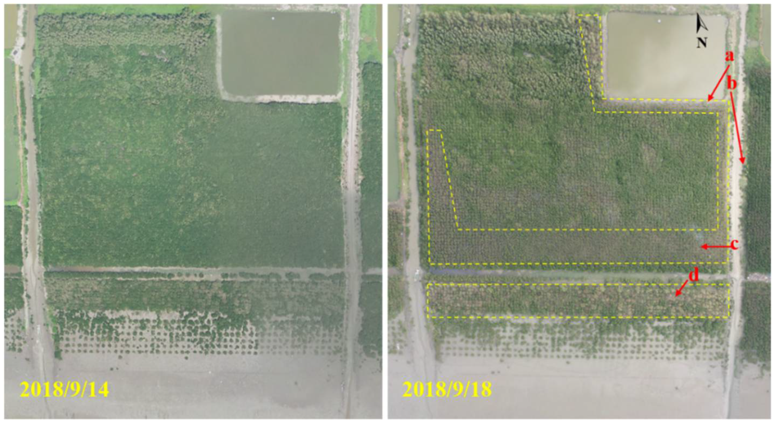
The study site (N22.83°, E115.21°) was located on the coast of Shanwei, Guangdong, China (Figure 1a). The planted mangrove forest is located along the coast of a lagoon in Honghai wan and is 13 km west of the Shanwei tide station (Figure 1b). In order to quantify the coastal protection provided by mangroves and understand the resilience of the planted mangrove trees against intense coastal storms, a field survey was conducted from 14 to 18 September 2018, during which the study site was heavily affected by super typhoon Mangkhut (Figure 1a). The track and intensity of typhoon Mangkhut were obtained from the National Meteorological Center of the China Meteorological Administration (CMA). The storm decayed to a severe typhoon after it left the Philippines and stayed as a severe typhoon until it made its second landfall at Jiangmen, Guangdong, China, at around 5 p.m. on 16 September 2018 (G.M.T + 8 time). The maximum wind speed at the typhoon central exceeded 45 m/s (level 14), and the lowest pressure in the center was 955 hPa upon landfall. During the typhoon event, the observed storm surge was 1.5 m, and the significant wave height was up to 9 m in the open sea in the Pear River Estuary, Guangdong, China [38], which is located 200 km southwest of the present study site. The study site entered the level 7 wind circle (520 km from the typhoon center) at 7 p.m., September 15, and was directly affected by the typhoon winds for the next 24 h. The shortest distance from the study site to the track of typhoon Mangkut was 200 km, within a level 10 wind circle. During the influence of typhoon Mangkhut, the observed wind level reached 8 to 15 in Shanwei city. Strong gusts of wind caused vast cases of traffic accidents, fallen trees, and damaged advertisement boards.

Funded by the local coastal restoration project, fast-growing mangrove species Laguncularia racemosa (dominant) and Sonneratia apetala were planted from 2012 to 2016, forming a 3.5 km long (in the alongshore direction) and 50 to 250 m wide (in the cross-shore direction) mangrove forest (Figure 1c). Small trees, about 1 m in height, were planted in a 2 m × 2 m (at the shore side) and 4 m × 4 m (at the offshore side) square pattern, forming three plant regions from the shore to the offshore side, i.e., a 108 m wide dense Laguncularia racemosa (blue-line bounded region, 2500 plants/ha), a 21 m wide Sonneratia apetala (red-line bounded region, 2500 plants/ha), and 26 m wide sparse Laguncularia racemosa (black-line bounded region, 625 plants/ha) (Figure 1d). The reason to use small trees instead of seeds, which is much cheaper, was because the seedlings are vulnerable to tidal currents and wind waves, as well as fast sedimentation in the early stage of growth. First, the roots of the seedlings may not be well developed to stand against tidal currents and wind waves. Second, the newly germinated seedlings can be too short and might be buried by fast sedimentation; this mechanism was supported by our field observations (Section 3.5).

To provide a reference for the mangrove’s protection, we made an exceptional effort to identify the structural details and quantify the plant’s geometric dimensions. Specifically, the plant height, length, and diameter of the stem, branch, twig, leaf, and above-ground root of 5 trees near stations B, C, and D were measured for each species. The size of the specimen corresponds to a minimum desired margin of error MOE = 0.9σ (σ is the standard deviation) for 95% CI (Confidence Interval) and MOE = 0.6σ for 80% CI considering a standard normal distribution [39]. Sonneratia apetala stands as individual trees (Figure 2a-1); each has a short trunk and is separated into two to five stems within 20 cm above the mud surface (e.g., illustrated in Figure 2a-3). The multi-stemmed Laguncularia racemosa presents in clusters (Figure 2b-1). Each cluster of Laguncularia racemosa plant has N_s stems separately emerged from the mud; one illustration of the Laguncularia racemosa stem is shown in Figure 2b-3.

The statistical properties for the measured plant’s geometric dimensions, including stem, branch, twig, leaf, and above-ground root (i.e., pneumatophore for Sonneratia apetala) are summarized in

Table 1. Measured plant properties, h_p is the plant height, N_s is the number of stems for one plant. D, L, and W are the diameter, length, and width of the plant element, respectively, with the subscript s, B, T, l, and r denoting the stem, branch, twig, leaf, and root (pneumatophore), respectively, S denote the space between two neighbor elements. N_l is the number of leaves on one twig (e.g., shown in Figure 2b-2). N_r is the density of pneumatophore.

Parameters	Laguncularia racemosa			Sonneratia apetala
	Mean ± Std	Min–Max	Samplings	Mean ± Std	Min–Max	Samplings
hp (m)	3.04 ± 0.86	1.4–4.8	14	4.00 ± 0.95	2.7–5.2	5
Ns (per plant)	29 ± 10	19–39	4	3.2 ± 1.3	2–5	5
Ds (mm)	14.6 ± 11.5	4–61	115	79 ± 20	46–131	16
LB (cm)	92 ± 26	58–128	16	195 ± 62	142–335	11
DB (mm)	11.7 ± 3.6	6.9–15.6	16	44 ± 10	31–61	16
SB (cm)	11.9 ± 4.5	7–22	16	17 ± 11	6–47	16
LT (cm)	32 ± 12	19–50	6	109 ± 20	72–132	8
DT (mm)	4.7 ± 2.7	2–8	6	21 ± 6	13–31	16
ST (cm)	7 ± 3	3–10	6	19 ± 9	4–38	16
Nl (per twig)	13 ± 3	8–18	6	169 ± 64	64–256	16
Ll (cm)	8.0 ± 1.4	6.4–10.6	16	7.7 ± 1.0	6.4–10	16
Wl (cm)	3.4 ± 0.4	2.9–4.1	16	2.3 ± 0.3	1.8–2.7	16
Nr (m−2)				144 ± 28	122–186	4
hr (cm)				11 ± 3	7–18	16
Dr (mm)				9 ± 2	5–12	16

. First, for Laguncularia racemosa, each plant includes a cluster of 19 to 39 stems that emerge from the mudflat. The largest stem diameter ranged from 40 to 60 mm. Overall, 5 to 12 stems (8 on average) had stem diameters greater than 20 mm and were mature enough to generate branches. For stems with D_s < 20 mm, only twigs were shown. The branches emerged in pairs with an average diameter of 11.7 mm, and a branch length of 92 cm, the average space between the two pairs of branches was 11.9 cm. Small twigs were distributed in pairs along the branches, and each twig had 8 to 18 leaves, e.g., shown in Figure 2b-2. Second, for Sonneratia apetala, the average basal diameter of the trunk is 121 ± 42 mm (SD), which is separated into two to five stems within 20 cm above the mud surface (Figure 2a-3). Note that each Sonneratia apetala twig contains a few leaflets (e.g., one leaflet is shown in Figure 2a-2), and the total number of leaves (169 ± 64) is the sum of leaves on all these leaflets. The above-ground root (pneumatophore) density for Sonneratia apetala is 144 roots/m², and the mean height and diameter of the pneumatophores are 11 cm and 9 mm. No above-ground roots were observed for Laguncularia racemosa.

Based on the plant properties summarized in Table 1 and the idealized plant structure shown in Figure 2a-3,b-3, the vertical variation of the plant solid volume fraction (SVF) was estimated and it is shown in Figure 1e. The MATLAB code for the SVF is provided in Text S1 in the Supplementary Materials. The first 26 m wide sparse Laguncularia racemosa has the lowest vegetation density and the shortest plant height, associated with the lowest SVF value (less than 0.45%, black bars in Figure 1e). The SVF for the dense Laguncularia racemosa on the shoreside reached 1.7% (blue bars in Figure 1e). The Sonneratia apetala was obviously taller and thicker than Laguncularia racemosa and had a maximum SVF = 4.8% (red bars in Figure 1e). These plant solid volume fractions are comparable to the values reported for Avicennia marina mangrove on the coast of the South China Sea, along Leizhou bay (SVF = 0.76 to 1.53%, [40]) and for three mangrove species (Avicennia, Sonneratia, and Rhizophora) in the southern Andaman region of Thailand (SVF = 0.43 to 3.2%, [30]. The detailed plant properties reported here can be applied to build mimic models for flume experiments and estimate the forest resistant force under various hydrodynamic processes (as undertaken in [41]), which is a basic component in large-scale mangrove-storm wave numerical modeling.

2.2. Aerial Survey

The aerial surveys were conducted on 29 June, 14 September and 18 September to capture the morphology of the mangrove forest and the fish pond behind. The drone aerial photography was taken by a DJI Phantom 4 Pro camera, which used a 1-inch 20-megapixel CMOS sensor. When flying at a height of 100 m, the digital orthophoto images has a precision of 2.74 cm/pix. The drone photos were aligned and processed using Agisoft PhotoScan to build three-dimensional maps and orthophotos of the study area (e.g., Figure 1c). The orthophotos for 29 June and 14 September were compared to show the growth of vegetation and the changes in the tidal flat during the typhoon season. The orthophotos for 14 September and 18 September, representing the pre- and post-typhoon conditions, were compared to show the fish pond and embankment protection provided by the mangrove forest during typhoon Mangkhut and to show the impact of the typhoon event on the mangrove trees.

2.3. Hydrodynamic Survey

Four pressure gages were applied to measure the water level on a mudflat to the mangrove cross-shore transect at stations A, B, C, and D (Figure 1c). Due to the limitations of the available instruments, three types of pressure gages were applied, with an Aanderaa Seaguard WLR (Norway) pressure gage at station A, two RBRduet T.D|tide (Canada) pressure gages at stations B and C, and a YPS600-J (China) pressure gage at station D. Gage A collects 2048 pressure records continuously at 4 Hz every 10 min. Gages B and C collect pressure data continuously at 2 Hz, and gage D collects pressure data continuously at a 20 Hz sampling frequency. The basic properties of the pressure gages are summarized in

Table 2. Basic properties of the pressure gages used in the hydrodynamic survey.

Gage	Brand	Measuring Range	Sampling Rate	Storage	Continuous Working Time	Operating Temperature	Sensor Height from Bottom
A	Aanderaa Seaguard WLR (Norway)	0 to 60 Mpa	4 Hz	2 Gb	6 months	−4 to 36 °C	35 cm
B and C	RBRduet T.D|tide (Canada)	0 to 20 m	2 Hz	2 Gb	3 years	−5 to 35 °C	24 cm
D	YPS600-J (China)	0 to 3 m	20 Hz	8 Gb	120 h	−40 to 60 °C	2 cm

.

First, the atmospheric pressure, which equals the measured pressure when the sensor was emergent, was removed from the measured pressure data to obtain the hydraulic pressure, including the hydrostatic pressure (representing the water depth associated with the low-frequency tide and storm surge) and the dynamic wave pressure. Note that the pressure measurements at station C were applied to represent the atmospheric pressure for all stations because (1) station C was emergent for a longer duration than the other stations and (2) the lower pressures (which are equal or approximately equal to the atmospheric pressure) at stations A, B, and D collapsed to the pressure at station C within 2 cm water depth. When station C was also submerged (for about 8 h), a linear interpolation of the pressure under the emergent conditions was applied to estimate the corresponding atmospheric pressure. Second, spectrum analysis was used to separate the water depth and wave data from the hydraulic pressure. Specifically, the hydrostatic pressure was obtained by using a cutoff frequency of 1/600 Hz to the hydraulic pressure data and then used to calculate the water depth considering the vertical distance between the sensor and the bed (sensor height from bottom in Table 2). The wave data were represented by the high-frequency component (0.02 Hz ≤ f ≤ 20 Hz) of the hydraulic pressure, which was segmented into 10-min bursts to estimate the variation in wave characteristics. The maximum wave height H_max was obtained using the zero-crossing method. The significant wave height $H_{m0}$ and mean wave period $T_{m2}$ were obtained using the spectrum method described in [42,43],

$$H_{m0}=4\sqrt{m0}$$

(1)

$$T_{m2}=\sqrt{m0/m2}$$

(2)

in which m0 and m2 are the 0th and 2nd momentum of wave energy density E (m²/Hz), respectively, and calculated by,

$$mn={\displaystyle \int }E\left(f\right)f^{n}df$$

(3)

To avoid differences arising from the different sampling frequencies between the pressure gages, only the frequency component within 1 Hz was used to estimate mn. This is fare because the energy distributed above 1 Hz is less than 0.1% of the total wave energy (e.g., Figure S1 in the Supplementary Materials).

The wave height decay can be expressed as $H_l/H_0=1/\left(1+\alpha l\right)$ [44], in which $H_0$ and $H_l$ are the wave height at a reference location and the wave height at l m behind, $\alpha$ is the reciprocal wave damping factor,

$$\alpha =\frac{H_0-H_l}{H_l\times l}$$

(4)

To facilitate wave attenuation over different vegetation widths and reported in different studies, the wave attenuation rate over 100 m is defined by $R_{w100}$,

$$R_{w100}=\frac{H_0-H_{100}}{H_0}=\frac{\alpha \times 100}{1+\alpha \times 100}$$

(5)

3. Results and Discussions

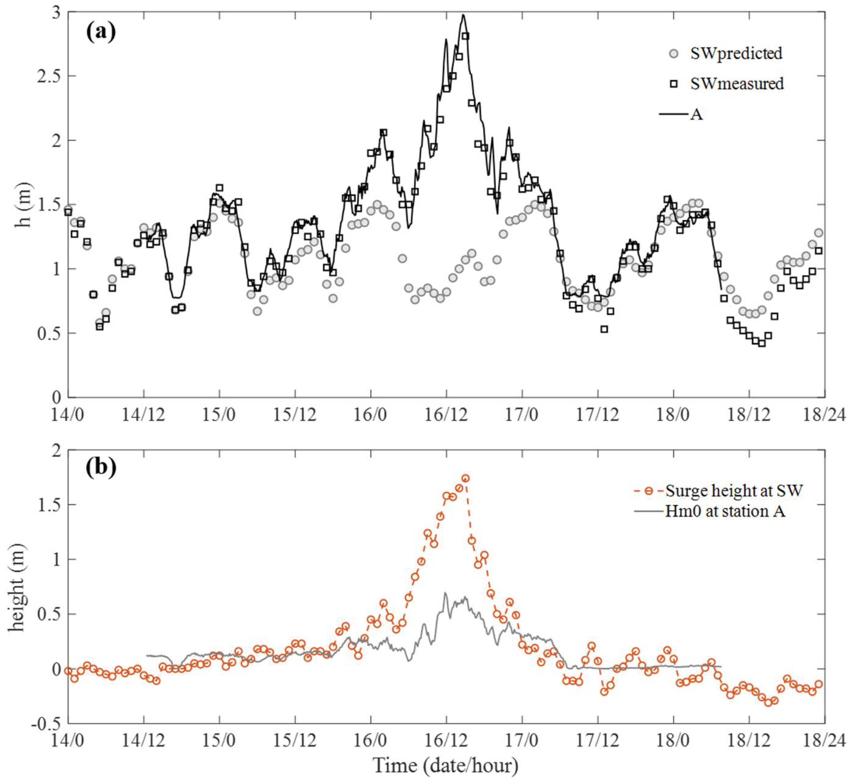
3.1. Tide Condition and Typhoon Influence

The predicted tide level and measured water depth at the Shanwei tide station (SW, 22°46′ N, 115°22′ E, 13 km east of the study site, as shown in Figure 1b) were plotted against the measured water depth at station A (Figure 3a). The predicted tide level and measured water depth for SW were obtained from http://global-tide.nmdis.org.cn/ (accessed on 15 December 2021), with the zero-elevation at 1 m below the mean sea level. The minimum root-mean-square error between the measured water depth at A and SW was 0.44 m, and this value has been added to the measured water depth at station A to exclude the difference that arose through the differences in the reference elevation between the two locations. Based on the predicted tide level and measured water depth at SW, typhoon Mangkhut induced an obvious storm surge from 15 to 17 September, with the maximum storm surge under higher water levels being 1.74 m at 3 p.m., 16 September (Figure 3b). Note that the minimum distance between the typhoon center and the study area was 200 km at 12 a.m., 16 September, and the typhoon made its landfall at 5 p.m., 16 September, at Jiangmen, Guangdong, China, which is 290 km from the study site.

The significant wave height at station A was plotted with the surge height at SW to show the impact of typhoon Mangkhut on the local wave conditions (Figure 3b). Specifically, the H_m0 at station A was positively related to the surge height, with H_m0 obviously larger during the influence of typhoon Mangkhut (before 7 a.m., 17 September) and became much smaller after the effects of the typhoon. As shown in Figure 1b, the mangrove forest is located in a lagoon with a narrow interface to the open sea, such that the flow field is generally calm and has a small wave height under normal tides and calm weather. However, during typhoon Mangkhut, the wave height at the study site was significantly amplified due to the propagation of offshore waves and the generation of local waves under strong storm winds. The obvious greater H_m0 during the typhoon would enhance sediment resuspension and motion, thus affecting the stability of the tidal flat [45]; this aspect will be discussed in more detail in Section 3.5.

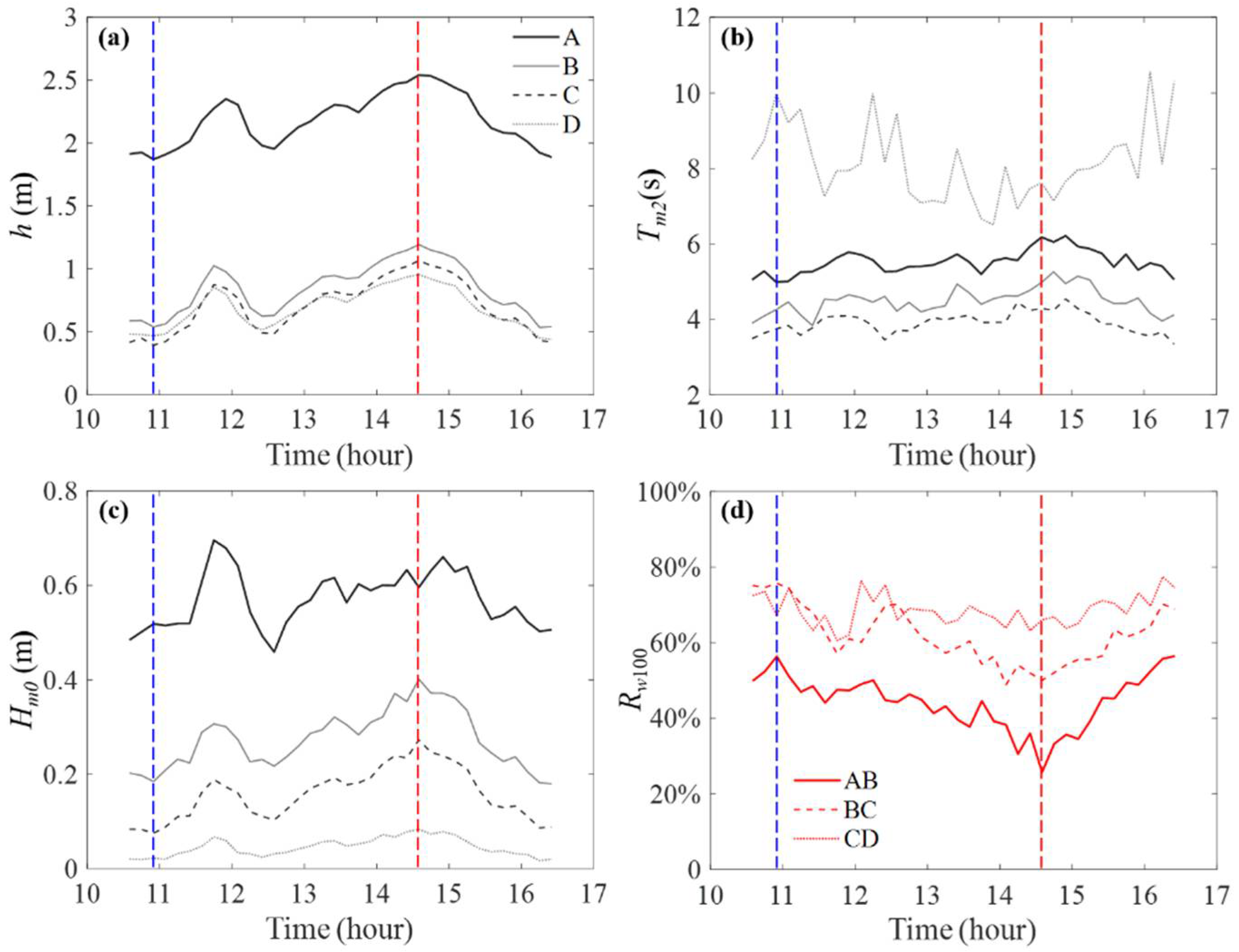
3.2. Wave Condition and Wave Attenuation

The measured wave conditions and the wave attenuation along the cross-shore transect were analyzed using the data from 10:30 to 16:30, 16 September, during which the water depth (relative to the local bed surface) at all four stations was greater than 0.4 m and the influence of typhoon was strongest (Figure 3). The characteristic wave parameters for each station over this time period are listed in

Table 3. Characteristic wave parameters for the measured stations for water depth h > 0.4 m, corresponding to time period from 10:30 to 16:30, 16 September. The subscript max, mean, and min indicate the maximum, mean and minimum value. T_m2 is the mean wave period. H_m0 is the significant wave height. The attenuation rate over 100 m (Equation (5)) was added between two adjacent stations and labeled by the ratios in red font.

Station	hmax (m)	hmean (m)	${\mathit{T}}_{\mathit{m}2} \left(\mathbf{s}\right)$	Hmax (m)	${\mathit{H}}_{\mathit{m}0} \left(\mathbf{m}\right)$	${\mathit{H}}_{\mathit{m}0}\mathbf{at}\mathit{h}\left(\mathbf{m}\right)$	${\mathit{H}}_{\mathit{m}0}\mathbf{at}\mathit{h}\left(\mathbf{m}\right)$
A	2.54	2.18	5.6	1.16	0.57	0.60	0.52
				33%	43%	26%	56%
B	1.19	0.84	4.6	0.69	0.28	0.40	0.18
				35%	59%	50%	76%
C	1.07	0.71	4.1	0.55	0.17	0.27	0.09
				77%	67%	66%	67%
D	0.96	0.69	7.8	0.11	0.05	0.08	0.02

. The time variation of the water depth h, the mean wave period $T_{m2}$, significant wave height $H_{m0}$, and the corresponding wave attenuation rates R_w100 were obtained using the 10-min data sets and are shown in Figure 4. The detailed data for each 10-min data set are summarized in Table S1 in the Supplementary Materials.

First, the water depth decreased continuously from station A to D (Figure 4a), with the decrease in h = 1.34 ± 0.03, 0.13 ± 0.01, 0.02 ± 0.06 m at reaches AB, BC, and CD, respectively. The greater fluctuation of the decreased water depth between CD might be caused by the differences in surge reduction due to the mangrove plant resistance. Based on the measurements and simulation within the unchanneled intact mangrove [11,46,47], the surge reduction might range from 1 to 8 cm over the 164 m wide cross-shore mangrove region (stations B to D). Note that the cross-shore tidal channels (Figure 1c) might have enhanced fluid transport in the cross-shore direction [48] and might be associated with a smaller surge reduction. Further, wave attenuation over the mangrove forest (Figure 4c), which reduces wave setup, might also contribute to the variation in water depth [49].

Second, the mean wave period $T_{m2}$ decreased from station A to C but was much greater at station D (Figure 4b). The opposite variation in $T_{m2}$ might be caused by two different mechanisms. The wave period reduction from station A to C was consistent with the nonlinear transfer of energy to higher frequencies, which was associated with a smaller mean wave period as the waves propagated over the mudflat–mangrove cross-shore transect [43,50]. Specifically, the breaking of incident waves, which was expected to occur over stations A and C, resulted in the greater energy distribution at higher frequencies and explained the reduction in the mean wave period. As an example, the 10-min wave signals at all four stations correspond to the deepest and shallowest water depth at station A (labeled by the red and blue vertical lines in Figure 4) are shown in Figure S2 in the Supplementary Materials. Specifically, the ratio of incident wave height to water depth at stations A to C can exceed 0.4, but within 0.16 at station D. According to the field study by Horstman et al. [30], waves tend to break at a threshold ratio of wave height to water depth = 0.4, suggesting that wave breaking might occur at reaches AB and BC, which lead to a reduction in the mean wave period from station A to C. However, no wave breaking was expected to occur at reach CD. The mangroves tend to attenuate shorter waves more efficiently than the longer waves [51]. Even within the range of infragravity waves (wave period between 25 and 250 s), low-frequency waves can propagate further toward the shore than high-frequency waves [52]. Our measurements also suggested that the mangrove can attenuate shorter waves (high-frequency waves) more efficiently than longer waves (low-frequency waves). Specifically, the ratio of energy distributed in the low-frequency part is greater at station D than at station C (Figure S1 in the Supplementary Materials), associated with a greater mean wave period in station D.

Third, the significant wave height was positively related to the water depth at all stations and it decreased continuously from station A to D (Figure 4c). The wave attenuation rate over 100 m $R_{w100}$ was 44% ± 7%, 62% ± 7%, and 69% ± 4% (SD) at reaches AB, BC, and CD, respectively (Figure 4d). The measured wave attenuation rates ranged in the upper bound of the previously reported wave damping rates for mangroves ($R_{w100}$ = 13% to 66%, reviewed in [53] and reported in [30,40]). Note that the $R_{w100}$ at the three reaches corresponded to different water depth, wave height, bottom slop, and with or without mangrove trees, and all of these parameters can significantly influence the attenuation rate. Specifically, the ratios of significant wave height to water depth were H_m0/h = 0.26 ± 0.01, 0.33 ± 0.02, 0.22 ± 0.02, and 0.06 ± 0.01 (SD), at stations A, B, C, and D, respectively. These H_m0/h values indicate that the breaking of incident waves, which can contribute to a large portion of energy loss under storm conditions [6], mainly occurred near station B. At reach AB, wave attenuation was caused by bottom friction and incident wave breaking (e.g., indicated by the incident wave height to water depth ratio in Figure S2 in the Supplementary Materials). At reach BC, except for bottom friction and incident wave breaking, the drag force due to mangrove plant structures added to the attenuation rate. At reach CD, the small H_m0/h ratio indicates no wave breaking, and the greatest wave attenuation was mainly caused by the strong resistance of the dense mangrove plants. Further, the bottom slop (S) is greater over AB (S = 0.96%) than BC (S = 0.27%) and CD (S = 0.09%), which was associated with a greater wave reduction [54], might, to some degree, have reduced the difference in $R_{w100}$ over the three reaches.

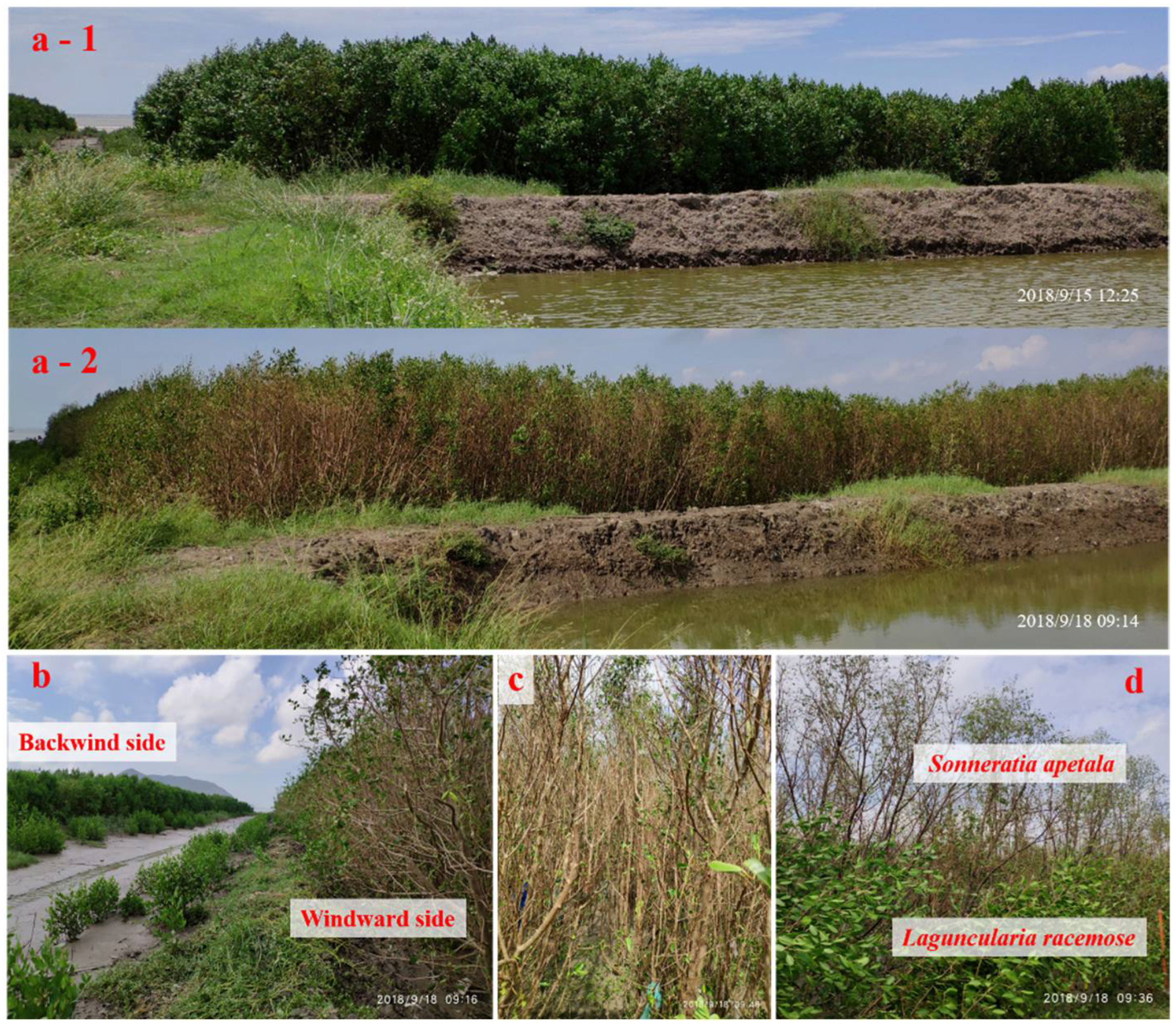
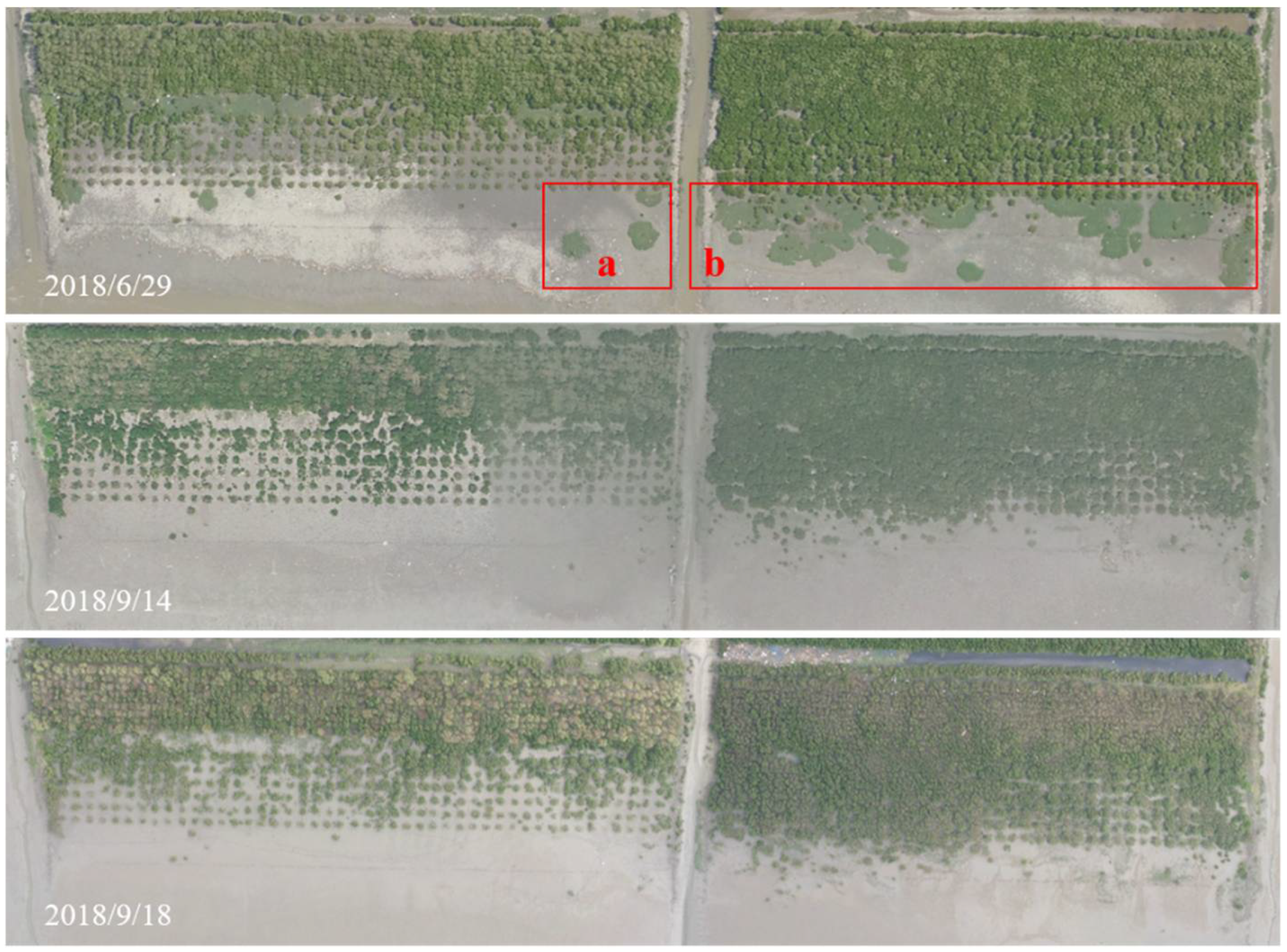
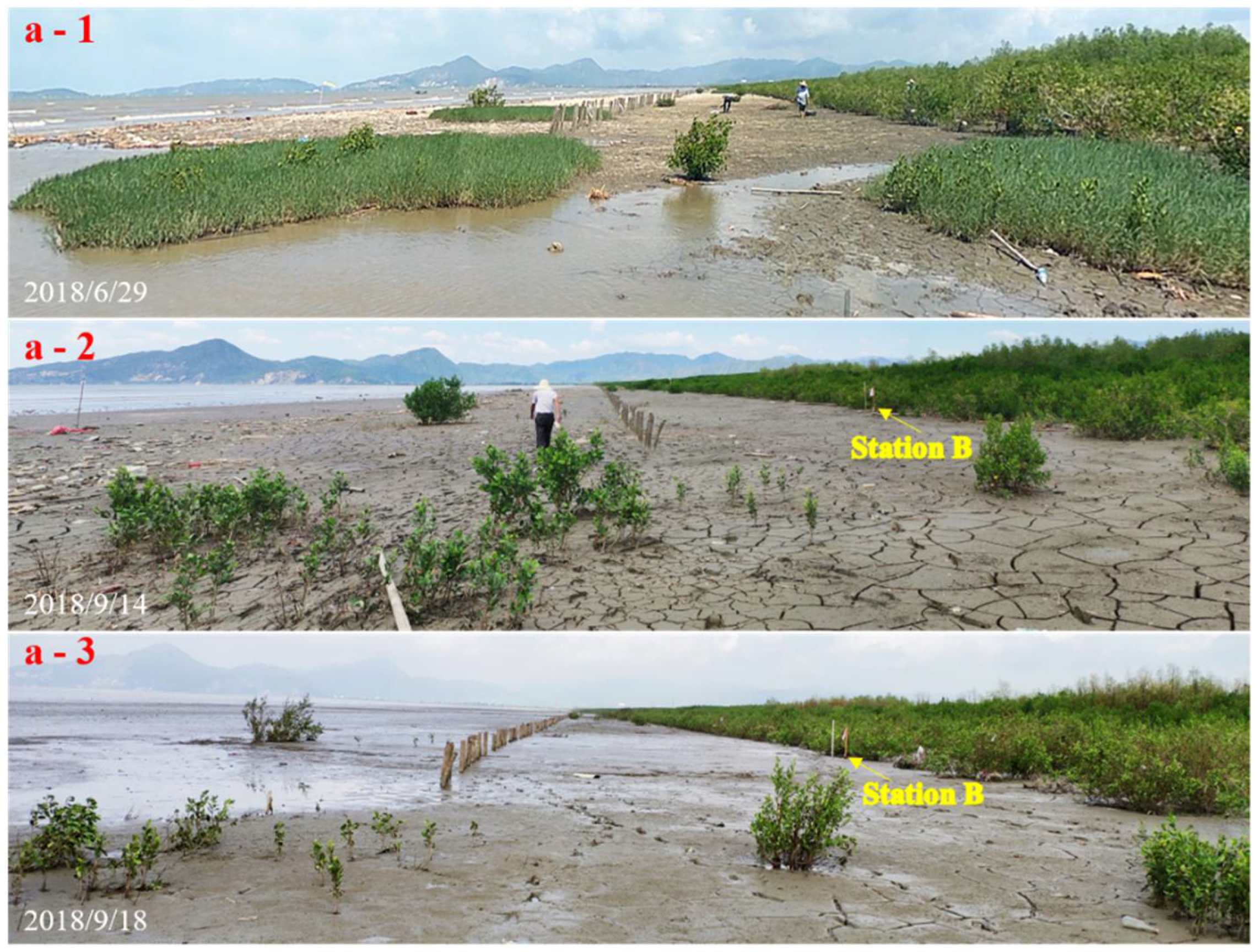
3.3. Resilience of Planted Mangrove to Intense Storm

No severe damage to mangrove trees (e.g., breaking of trunks and uprooting of trees) was found in our survey, while a few individual broken branches and common defoliation were spotted within the mangrove forest, especially along the direction of the wind path, at the windward forest edges, and for the taller trees (e.g., the yellow-line bounded regions in Figure 5). First, along the direction of the wind path, mostly from east to west, the gusts of intense wind caused continuous defoliation (e.g., Figure 6a,c). Second, for mangrove trees along the two sides of the tidal channel, heavier defoliation occurred on the windward side of the mangrove forest, while the mangrove trees remind intact on the backwind side (e.g., Figure 6b). Third, the taller Sonneratia apetala experienced severer defoliation compared to the shorter Laguncularia racemosa plants at the same location (e.g., Figure 6d), which is consistent with previous field surveys that demonstrated that the larger trees were more likely to be damaged, and damaged more severely than smaller trees [55,56]. The greater exposure surface and more frequent wind perturbation of the larger plants might explain the severer defoliation. Note that for similar plant heights, the trees with bigger trunks are less vulnerable to storm breakage [57,58].

Although both the intense wind and the storm waves could damage the plants, the wind contributed most to the plant defoliation in the present study. Recall that the wind level reached 8 to 15 in Shanwei city, where the study site was located. The waves did not contribute much to plant damage at the present site. First, the water depth and wave measurements shown in Figure 4a,c indicate h + H_m0/2 < 1.5 m at reach BD, suggesting that waves can only affect the plants up to 1.5 m above the mud surface. The waves did not cause upper-canopy defoliation because the tree height was generally 3 to 4 m (see Figure 1f). Second, the short, young seedlings, which were fully submerged and exposed to strong waves during the storm, remained in good condition (e.g., the seedlings in front of the mangrove and in the tide channel, see Figure 6b and Figure 9a-3).

In contrast, the damage to mangrove plants on the southwestern coast of Florida due to hurricane Andrew (24 August 1992, surveyed by [56]) was much more severe, inducing 85% uprooting, breakage, and death of trees. Except for the smaller plant size, the denser forest and less intense wind also contributed to less damage in the present survey (with most areas being 2500 plants/ha and a maximum wind speed of 45 m/s at the typhoon center). Specifically, the mangroves on the southwestern coast of Florida had a 9.2 cm mean diameter at breast height and a density of 1903 plants/ha. The wind speed during hurricane Andrew exceeded 67 m/s. Another field survey reported 97% mangrove tree defoliation and uprooting along the Caribbean coast due to extreme winds up to 108 m/s during hurricane Mitch (1998) [59]. Note that the waves might also contribute to plant damage at these sites. However, no wave data were reported in these studies.

Except for the storm’s wind and wave intensity, the potential of storm resilience of mangroves varied among plant species. Specifically, the mechanical strength and flexibility of the branches, leaves, and stems also affect the degree of damage among different plant species during storm events [60]. Some mangrove species can recover within a relatively short period of time after severe storm damage, while others may recover poorly. For example, Avicennia and Sonneratia showed a greater ability to withstand strong storm impacts, while plant refoliation and seedling regeneration were better than Rhizophora [61]. The heavily defoliated Sonneratia alba plants in Eastern Samar sprouted four-and-a-half months after the 2013 typhoon Haiyan [62]. In the Everglades National Park, United States, severe die-off mangrove forests were observed to recover to pre-storm levels 3 to 4 years after storm events [63].

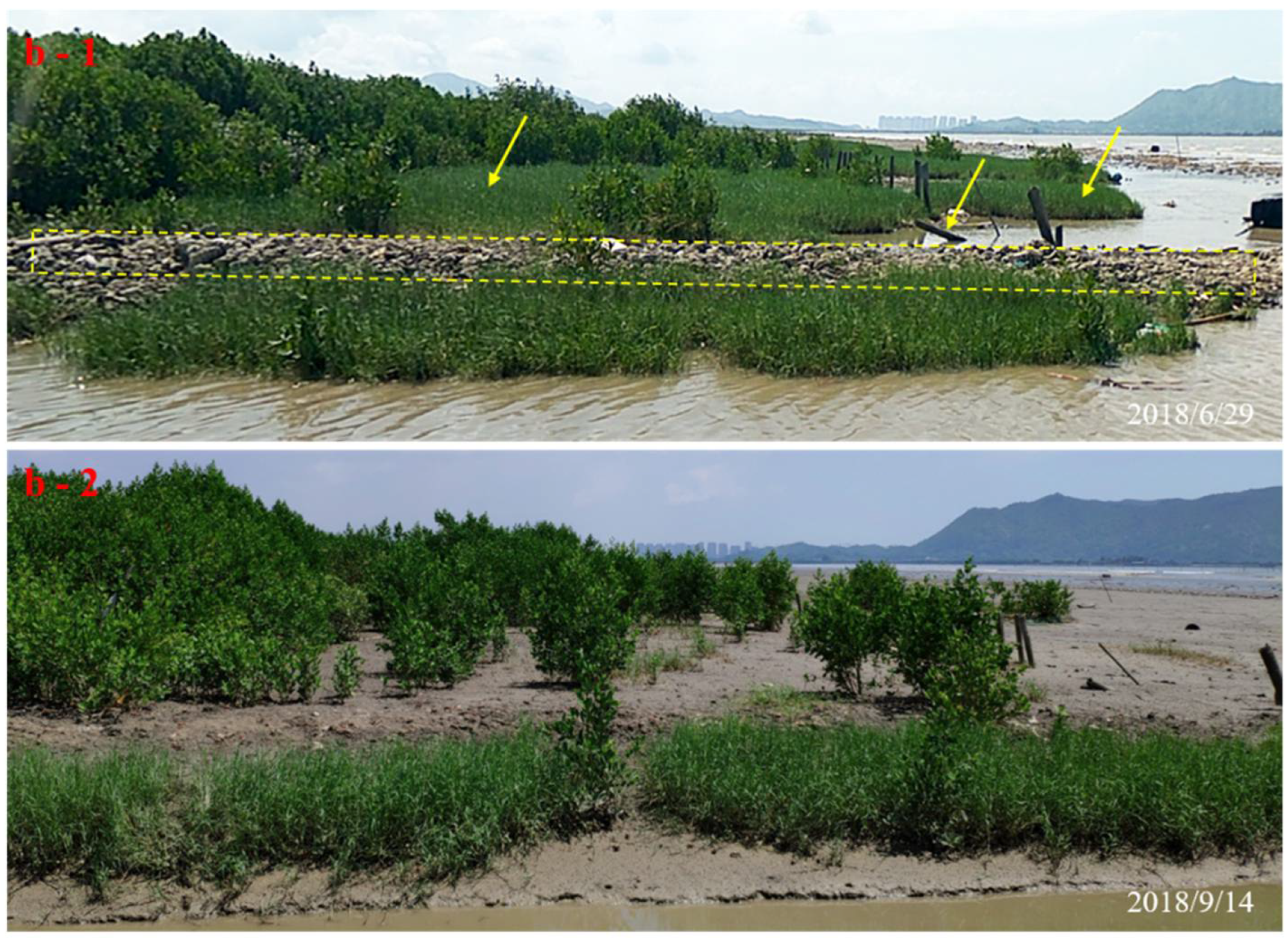
3.4. Protection of Fish Ponds and Embankments by Mangroves during Storms

The fishponds and embankments behind the mangroves reminded intact during typhoon Mangkhut according to the pre- and post-typhoon aerial and ground survey. However, just outside the western edge of the mangroves, e.g., the yellow-line bounded area shown in Figure 1c, obvious breakage was observed along the embankments (Figure 7). Further west from the mangrove forest, the embankments were also eroded in a few places. The obvious opposite finding of the embankments with and without mangroves on the offshore side has also been reported by [12], suggesting that the mangroves provided protection to the embankments behind. The presence of mangroves could contribute to flow resistance and reduce wind and swell waves (as in [7] and in Section 3.2 in the present study), decrease current velocity [8,9], and mitigate storm surges [9,11], all of which lead to a smaller hydrodynamic force acting on the embankment and less wave overtopping and flooding, which is associated with a lower tendency and degree of embankment breaches. Wind waves were recognized as a major cause of structural damage in Tacloban, Philippines, during Typhoon Haiyan (2013) [64]. Similarly, for the current site, the protection of the fishpond and embankment was mainly attributed to the wave reduction due to the mangroves, while the storm surge height was estimated to be reduced by 1 to 8 cm by the narrow mangrove forest.

3.5. Coastal Sedimentation and Erosion Prevention within Mangroves

One of the interesting findings of the survey is that the front region of the mangrove (both the sparse Laguncularia racemosa region and the mudflat) experienced fast sedimentation during the time period from 29 June to 14 September (Figure 8). Two of the most obvious pieces of evidence are shown in the red boxes a and b in Figure 8, within which the Laguncularia racemosa seedlings and salt grasses were grown together on 29 June. However, the pre-typhoon survey on 14 September showed no salt grasses but only mangrove seedlings because the salt grasses were buried by sedimentation. A closer comparison of regions a and b is shown in Figure 9 and Figure 10, respectively. Specifically, during the first survey (29 June to 1 July), the salt grasses were about 20 to 30 cm in height, which was comparable to the height of some of the small seedlings (Figure 9a-1 and Figure 10b-1). At the beginning of the second survey (September 14), only the mangrove seedlings were standing in regions a (Figure 9a-2) and b (Figure 10b-2). A rough test showed that the 20 cm surface soil was soft but quite hard further down in region a (Figure 8), suggesting that the 20 cm deep surface soil was newly deposited sediments. The burial of the salt grasses but not the mangrove seedlings can be explained by the greater plant flexibility in the salt grasses, as flexible plants bend under tidal currents and waves [65,66,67], which add to their vulnerability to sediment deposition. In this case, the sedimentation benefited the mangroves in competition with salt grasses. However, when the sedimentation rate exceeds the rate of mangrove seedling growth, they can be buried as well. Recent experiment examined seedlings’ accretion and erosion thresholds which showed that seedlings are likely to survival sediment accretion (10 out of 12 specimens) while, for some species, the seedlings can be negatively affected by sediment erosion [68].

Sediments can be brought to the mangrove region by massive flooding, upland erosion, and mud and debris flow. Mangrove forests can be severely damaged due to upland sediment burial during severe storm events. For example, driven by Hurricane Mitch (1998), vast sedimentation was reported to burry mangroves on the island of Guanaja by 1.2 m, as sand eroded from the nearby shorelines [59]. In the current survey, a comparison of the above-ground height of the iron posts (used to hold the sensors in place) at the stations before (14 September) and after the typhoon Mangkhut (18 September) showed a 7 cm sedimentation at station B (Figure 9a-2,a-3), but no obvious sedimentation at stations C and D. Fast sedimentation has also been observed in recent years by local farmers who participated in the planting of the mangrove forest. Specifically, the plants on the offshore edge were observed to be buried obviously after storm events and during the typhoon seasons. Based on the water level shown in Figure 3 and ignoring the wave runup-induced inundation, the minimum tide required to flood the mangrove area (at station B) is 1.5 m at SW, which occurred 11% of the time based on the predicted tide at SW during the year 2018. With the storm surge and wave runup during the typhoon season, the frequency of inundation can be much larger than 11% and bring excessive sedimentation to the front edge of the mangrove forest.

A recent study showed that macro-tidal conditions with a large sediment supply promote accretion along the mudflat and mangrove platforms [69]. The fast sedimentation in the offshore edge of the mangrove forest and the tidal flat ahead might be explained by sufficient sediment supply from the Huang Jiang River on the east side of the study area (Figure 1b) and stronger hydrodynamic conditions during the typhoon season. Sediments tended to deposit along the shore edge side when transported from the Huang Jiang River to the lagoon under calm tide and wave conditions (as expected in general weather conditions, e.g., the post-typhoon H_m0 at station A shown in Figure 3). These sediments would be resuspended and transported to the mangrove and tidal flat region by intense waves and current velocity under storm conditions. Considering the ability to accrete land vertically by enhancing sedimentation and by direct organic contributions, mangroves are increasingly advocated as an adaptation method for long-term coastal protection to cope with future sea level rise and, at the same time, to maintain the mangrove forests and their ecosystem services [70]. Since sedimentation was observed in both the mudflat and the mangrove front, the contribution of mangroves in promoting vertical accretion is still unknown. However, a modest estimation of the direct contribution of mangroves to the tidal flat vertical accretion was the burial of roots, trunks, and branches, which ranged from 0.4 to 4.8% based on the estimated solid volume fraction (the present study and references [30,40]). Leaf and branch litter also add to the mangrove’s vertical accretion directly. The mangroves also indirectly impact the maintenance\accretion of tidal flats through the interaction with current, waves, and sediment motion. Quantitative analysis of how the sediment supply, tide and wave environment, and mangrove forest characteristics affect land accretion is still lacking. The present study site was a common region with a river sediment supply and tidal flats with and without mangroves; hence, further research is advocated to minimize the current knowledge gap in the contribution of mangroves in the intertidal sediment balance and long-term coastal protection.

4. Conclusions

This paper presents field evidence that demonstrates that planted mangroves can effectively enhance coastal resilience to tropical storms. The results support nature-based coastal stabilization policies and encourage the usage of planting mangroves in coastal restoration and conservation projects. Quantitative wave-damping data could help coastal planners determine the scale and type of planted mangroves needed to mitigate expected wave attacks under future storm surges or sea-level increases and to decide the time needed for the planted mangroves to reach the desired protection ability.

First, our observations and measurements testified that a ~100 m wide two-to-six-year-old mangrove forest could provide substantial protection against intense storm events and strong wave conditions. Typhoon Mangkhut (2018) induced a storm surge up to 1.74 m at the study site, with a maximum water depth of 2.54 m and a maximum wave height of 1.16 m at 140 m on the offshore side of the mangrove forest. Our pre- and post-typhoon aerial and ground surveys showed that the fishponds and embankments sheltered by the mangroves remained intact, while obvious embankment breakage occurred outside the western edge of the mangrove forest. The wave attenuation rate over 100 m was 44% ± 7%, 62% ± 7%, and 69% ± 4% (SD) at reaches AB (mudflat on the offshore side of the mangrove), BC (the two-to-six-years-old mangrove trees on the seaward part of the forest), and CD (the six-year-old dense mangrove trees on the shoreward part of the forest), respectively (Figure 4d). These wave attenuation rates ranged in the upper bound of the previously reported wave damping rates for mangroves ($R_{w100}$ = 13% to 66%, reviewed in [53] and reported in [30,40]).

Second, our observations suggest that a newly planted mangrove forest (two to six years old) can withstand intense typhoon impacts with only a small portion of severe defoliation and no deadly breakage or the uprooting of plants, demonstrating the high resilience of planted mangroves to intense storm disturbance. Specifically, no uproots or deadly breakage were observed in the mangrove trees due to the effects of Typhoon Mangkhut (2018), while severe defoliation occurred for a small portion of trees in the study area, mainly along the wind path, the windward edge of the forest, and among the taller plants. Note that the study site was 200 km northeast of the typhoon center when the typhoon passed through the region.

Third, except for direct observations and hydrodynamic measurements, the detailed structural and geometric dimensions of the plants were also measured to provide a reference for mangrove protection. The structural and geometric dimensions of the plants were scarce in previous studies, and such detailed data can be applied to build mimic model plants for future flume experiments/numerical simulations and to estimate the forest resistant force under various hydrodynamic conditions.

Finally, a 7 cm sedimentation was observed at the seaward edge of the mangrove forest (station B) during the impact of Typhoon Mangkhut (2018), and a 20 cm sedimentation at the front part of the mangrove and the tidal flat during the typhoon season in the year 2018. Vertical accretion is an important aspect of mangrove ecosystems, linking short-term coastal protection to long-term mangrove maintenance and their ecosystem functions, which should be viewed as a focal point in future studies.

References

1. Mitra, A. Mangrove Forests in India: Exploring Ecosystem Services; Springer International Publishing: Cham, Switzerland, 2020; ISBN 978-3-030-20594-2. [Google Scholar]
2. Donato, D.C.; Kauffman, J.B.; Murdiyarso, D.; Kurnianto, S.; Stidham, M.; Kanninen, M. Mangroves among the Most Carbon-Rich Forests in the Tropics. Nat. Geosci. 2011, 4, 293–297. [Google Scholar] [CrossRef]
3. Pendleton, L.; Donato, D.C.; Murray, B.C.; Crooks, S.; Jenkins, W.A.; Sifleet, S.; Craft, C.; Fourqurean, J.W.; Kauffman, J.B.; Marbà, N.; et al. Estimating Global “Blue Carbon” Emissions from Conversion and Degradation of Vegetated Coastal Ecosystems. PLoS ONE 2012, 7, e43542. [Google Scholar] [CrossRef] [PubMed]
4. Akber, M.A.; Patwary, M.M.; Islam, M.A.; Rahman, M.R. Storm Protection Service of the Sundarbans Mangrove Forest, Bangladesh. Nat. Hazards 2018, 94, 405–418. [Google Scholar] [CrossRef]
5. Koh, H.; Teh, S.; Kh’ng, X.; Raja Barizan, R. Mangrove Forests: Protection against and Resilience to Coastal Disturbances. JTFS 2018, 30, 446–460. [Google Scholar] [CrossRef]
6. Lee, W.K.; Tay, S.H.X.; Ooi, S.K.; Friess, D.A. Potential Short Wave Attenuation Function of Disturbed Mangroves. Estuar. Coast. Shelf Sci. 2021, 248, 106747. [Google Scholar] [CrossRef]
7. Mazda, Y.; Magi, M.; Ikeda, Y.; Kurokawa, T.; Asano, T. Wave Reduction in a Mangrove Forest Dominated by Sonneratia sp. Wetl. Ecol. Manag. 2006, 14, 365–378. [Google Scholar] [CrossRef]
8. Quartel, S.; Kroon, A.; Augustinus, P.G.E.F.; Van Santen, P.; Tri, N.H. Wave Attenuation in Coastal Mangroves in the Red River Delta, Vietnam. J. Asian Earth Sci. 2007, 29, 576–584. [Google Scholar] [CrossRef]
9. Dasgupta, S.; Islam, M.S.; Huq, M.; Huque Khan, Z.; Hasib, M.R. Quantifying the Protective Capacity of Mangroves from Storm Surges in Coastal Bangladesh. PLoS ONE 2019, 14, e0214079. [Google Scholar] [CrossRef]
10. Mullarney, J.C.; Henderson, S.M.; Reyns, J.A.H.; Norris, B.K.; Bryan, K.R. Spatially Varying Drag within a Wave-Exposed Mangrove Forest and on the Adjacent Tidal Flat. Cont. Shelf Res. 2017, 147, 102–113. [Google Scholar] [CrossRef]
11. McIvor, A.; Spencer, T.; Möller, I.; Spalding, M. Storm Surge Reduction by Mangroves; Natural Coastal Protection Series: Report 2; Cambridge Coastal Research Unit Working Paper 41; University of Cambridge: Cambridge, UK, 2012. [Google Scholar]
12. Badola, R.; Hussain, S.A. Valuing Ecosystem Functions: An Empirical Study on the Storm Protection Function of Bhitarkanika Mangrove Ecosystem, India. Environ. Conserv. 2005, 32, 85–92. [Google Scholar] [CrossRef]
13. Mazda, Y.; Magi, M.; Kogo, M.; Hong, P.N. Mangroves as a Coastal Protection from Waves in the Tong King Delta, Vietnam. Mangroves Salt Marshes 1997, 1, 127–135. [Google Scholar] [CrossRef]
14. Koh, H.L.; Teh, S.Y.; Liu, P.L.; Ismail, A.I.M.; Lee, H.L. Simulation of Andaman 2004 Tsunami for Assessing Impact on Malaysia. J. Asian Earth Sci. 2009, 36, 74–83. [Google Scholar] [CrossRef]
15. Gedan, K.B.; Kirwan, M.L.; Wolanski, E.; Barbier, E.B.; Silliman, B.R. The Present and Future Role of Coastal Wetland Vegetation in Protecting Shorelines: Answering Recent Challenges to the Paradigm. Clim. Chang. 2011, 106, 7–29. [Google Scholar] [CrossRef]
16. Horstman, E.M.; Dohmen-Janssen, C.M.; Bouma, T.J.; Hulscher, S.J.M.H. Tidal-Scale Flow Routing and Sedimentation in Mangrove Forests: Combining Field Data and Numerical Modelling. Geomorphology 2015, 228, 244–262. [Google Scholar] [CrossRef]
17. Van Santen, P.; Augustinus, P.G.E.F.; Janssen-Stelder, B.M.; Quartel, S.; Tri, N.H. Sedimentation in an Estuarine Mangrove System. J. Asian Earth Sci. 2007, 29, 566–575. [Google Scholar] [CrossRef]
18. Alongi, D.M. Mangrove Forests: Resilience, Protection from Tsunamis, and Responses to Global Climate Change. Estuar. Coast. Shelf Sci. 2008, 76, 1–13. [Google Scholar] [CrossRef]
19. McIvor, A.; Spencer, T.; Möller, I.; Spalding, M. The Response of Mangrove Soil Surface Elevation to Sea Level Rise; Natural Coastal Protection Series: Report 3; Cambridge Coastal Research Unit Working Paper 42; University of Cambridge: Cambridge, UK, 2013; p. 59. [Google Scholar]
20. Duarte, C.M.; Losada, I.J.; Hendriks, I.E.; Mazarrasa, I.; Marbà, N. The Role of Coastal Plant Communities for Climate Change Mitigation and Adaptation. Nat. Clim Chang. 2013, 3, 961–968. [Google Scholar] [CrossRef]
21. Morris, R.; Strain, E.M.A.; Konlechner, T.M.; Fest, B.J.; Kennedy, D.M.; Arndt, S.K.; Swearer, S.E. Developing a Nature-Based Coastal Defence Strategy for Australia. Aust. J. Civ. Eng. 2019, 17, 167–176. [Google Scholar] [CrossRef]
22. Morris, R.L.; Konlechner, T.M.; Ghisalberti, M.; Swearer, S.E. From Grey to Green: Efficacy of Eco-Engineering Solutions for Nature-Based Coastal Defence. Glob. Chang. Biol. 2018, 24, 1827–1842. [Google Scholar] [CrossRef]
23. Chang, C.-W.; Mori, N. Green Infrastructure for the Reduction of Coastal Disasters: A Review of the Protective Role of Coastal Forests against Tsunami, Storm Surge, and Wind Waves. Coast. Eng. J. 2021, 63, 370–385. [Google Scholar] [CrossRef]
24. Spalding, M.; Mcivor, A.; Tonneijck, F.; Tol, S.; van Eijk, P. Mangroves for Coastal Defence. In Guidelines for Coastal Managers & Policy Makers; University of Cambridge: Cambridge, UK, 2014. [Google Scholar]
25. McIvor, A.; Spencer, T.; Spalding, M.; Lacambra, C.; Möller, I. Mangroves, Tropical Cyclones, and Coastal Hazard Risk Reduction. In Coastal and Marine Hazards, Risks, and Disasters; Elsevier: Amsterdam, The Netherlands, 2015; pp. 403–429. ISBN 978-0-12-396483-0. [Google Scholar]
26. Van Coppenolle, R. Potenties Voor Natuur Gebaseerde Mitigatie Van Overstromingsrisico’s in Kustgebieden Een Regionale Tot Globale Studie; University of Antwerp: Antwerp, Belgium, 2018. [Google Scholar]
27. Yudha, R.P. Forest Structure of 26-Year-Old Planted Mangroves. J. Sylva Indones. 2021, 4, 61–69. [Google Scholar] [CrossRef]
28. Bouma, T.J.; van Belzen, J.; Balke, T.; Zhu, Z.; Airoldi, L.; Blight, A.J.; Davies, A.J.; Galvan, C.; Hawkins, S.J.; Hoggart, S.P.G.; et al. Identifying Knowledge Gaps Hampering Application of Intertidal Habitats in Coastal Protection: Opportunities & Steps to Take. Coast. Eng. 2014, 87, 147–157. [Google Scholar] [CrossRef]
29. Vo Luong, P.; Massel, S. Experiments on Wave Motion and Suspended Sediment Concentration at Nang Hai, Can Gio Mangrove Forest, Southern Vietnam. Oceanologia 2006, 48, 23–40. [Google Scholar]
30. Horstman, E.M.; Dohmen-Janssen, C.M.; Narra, P.M.F.; van den Berg, N.J.F.; Siemerink, M.; Hulscher, S.J.M.H. Wave Attenuation in Mangroves: A Quantitative Approach to Field Observations. Coast. Eng. 2014, 94, 47–62. [Google Scholar] [CrossRef]
31. Mori, N.; Chang, C.-W.; Inoue, T.; Akaji, Y.; Hinokidani, K.; Baba, S.; Takagi, M.; Mori, S.; Koike, H.; Miyauchi, M.; et al. Parameterization of Mangrove Root Structure of Rhizophora Stylosa in Coastal Hydrodynamic Model. Front. Built Environ. 2022, 7, 782219. [Google Scholar] [CrossRef]
32. Yoshikai, M.; Nakamura, T.; Suwa, R.; Argamosa, R.; Okamoto, T.; Rollon, R.; Basina, R.; Primavera-Tirol, Y.H.; Blanco, A.C.; Adi, N.S.; et al. Scaling Relations and Substrate Conditions Controlling the Complexity of Rhizophora Prop Root System. Estuar. Coast. Shelf Sci. 2021, 248, 107014. [Google Scholar] [CrossRef]
33. Sippo, J.Z.; Lovelock, C.E.; Santos, I.R.; Sanders, C.J.; Maher, D.T. Mangrove Mortality in a Changing Climate: An Overview. Estuar. Coast. Shelf Sci. 2018, 215, 241–249. [Google Scholar] [CrossRef]
34. Spencer, T.; Möller, I. Mangrove Systems. In Treatise on Geomorphology; Elsevier: Amsterdam, The Netherlands, 2013; pp. 360–391. ISBN 978-0-08-088522-3. [Google Scholar]
35. Jimenez, J.; Lugo, A.; Cintron, G. Tree Mortality in Mangrove Forests. Biotropica 1985, 17, 177. [Google Scholar] [CrossRef]
36. Paling, E.I.; Kobryn, H.T.; Humphreys, G. Assessing the Extent of Mangrove Change Caused by Cyclone Vance in the Eastern Exmouth Gulf, Northwestern Australia. Estuar. Coast. Shelf Sci. 2008, 77, 603–613. [Google Scholar] [CrossRef]
37. Cahoon, D.; Hensel, P.; Rybczyk, J.; McKee, K.; Proffitt, E.; Perez, B. Mass Tree Mortality Leads to Mangrove Peat Collapse at Bay Islands, Honduras after Hurricane Mitch. J. Ecol. 2003, 91, 1093–1105. [Google Scholar] [CrossRef]
38. Luo, Z.; Huang, B.; Chen, X.; Tan, C.; Qiu, J.; Huang, G. Effects of Wave–Current Interaction on Storm Surge in the Pearl River Estuary: A Case Study of Super Typhoon Mangkhut. Front. Mar. Sci. 2021, 8, 692359. [Google Scholar] [CrossRef]
39. Rumsey, D.J. How to Determine the Minimum Size Needed for a Statistical Sample. In Statistics for Dummies; Wiley: Hoboken, NJ, USA, 2016; ISBN 978-1-119-29352-1. [Google Scholar]
40. Cao, H.; Chen, Y.; Tian, Y.; Feng, W. Field Investigation into Wave Attenuation in the Mangrove Environment of the South China Sea Coast. J. Coast. Res. 2016, 322, 1417–1427. [Google Scholar] [CrossRef]
41. Maza, M.; Lara, J.L.; Losada, I.J. Predicting the Evolution of Coastal Protection Service with Mangrove Forest Age. Coast. Eng. 2021, 168, 103922. [Google Scholar] [CrossRef]
42. Zhang, X.; Lin, P.; Gong, Z.; Li, B.; Chen, X. Wave Attenuation by Spartina Alterniflora under Macro-Tidal and Storm Surge Conditions. Wetlands 2020, 40, 2151–2162. [Google Scholar] [CrossRef]
43. Jadhav, R.S.; Chen, Q.; Smith, J.M. Spectral Distribution of Wave Energy Dissipation by Salt Marsh Vegetation. Coast. Eng. 2013, 77, 99–107. [Google Scholar] [CrossRef]
44. Dalrymple, R.A.; Kirby, J.T.; Hwang, P.A. Wave Diffraction Due to Areas of Energy Dissipation. J. Waterw. Port Coast. Ocean Eng. 1984, 110, 67–79. [Google Scholar] [CrossRef]
45. Green, M.O.; Coco, G. Review of Wave-Driven Sediment Resuspension and Transport in Estuaries. Rev. Geophys. 2014, 52, 77–117. [Google Scholar] [CrossRef]
46. Krauss, K.W.; Doyle, T.W.; Doyle, T.J.; Swarzenski, C.M.; From, A.S.; Day, R.H.; Conner, W.H. Water Level Observations in Mangrove Swamps during Two Hurricanes in Florida. Wetlands 2009, 29, 142–149. [Google Scholar] [CrossRef]
47. Zhang, K.; Liu, H.; Li, Y.; Xu, H.; Shen, J.; Rhome, J.; Smith, T.J., III. The Role of Mangroves in Attenuating Storm Surges. Estuar. Coast. Shelf Sci. 2012, 102, 11–23. [Google Scholar] [CrossRef]
48. Montgomery, J.M.; Bryan, K.R.; Horstman, E.M.; Mullarney, J.C. Attenuation of Tides and Surges by Mangroves: Contrasting Case Studies from New Zealand. Water 2018, 10, 1119. [Google Scholar] [CrossRef]
49. Paquier, A.-E.; Haddad, J.; Lawler, S.; Ferreira, C.M. Quantification of the Attenuation of Storm Surge Components by a Coastal Wetland of the US Mid Atlantic. Estuaries Coasts 2017, 40, 930–946. [Google Scholar] [CrossRef]
50. Peng, Z.; Zou, Q.; Reeve, D.; Wang, B. Parameterisation and Transformation of Wave Asymmetries over a Low-Crested Breakwater. Coast. Eng. 2009, 56, 1123–1132. [Google Scholar] [CrossRef]
51. Harada, K.; Imamura, F. Effects of Coastal Forest on Tsunami Hazard Mitigation—A Preliminary Investigation. In Tsunamis; Satake, K., Ed.; Springer: Dordrecht, The Netherlands, 2005; Volume 23, pp. 279–292. [Google Scholar]
52. Mendes, D.; Fortunato, A.B.; Bertin, X.; Martins, K.; Lavaud, L.; Nobre Silva, A.; Pires-Silva, A.A.; Coulombier, T.; Pinto, J.P. Importance of Infragravity Waves in a Wave-Dominated Inlet under Storm Conditions. Cont. Shelf Res. 2020, 192, 104026. [Google Scholar] [CrossRef]
53. McIvor, A.; Möller, I.; Spencer, T.; Spalding, M. Reduction of Wind and Swell Waves by Mangroves; Natural Coastal Protection Series: Report 1; Cambridge Coastal Research Unit Working Paper 40; University of Cambridge: Cambridge, UK, 2012. [Google Scholar]
54. Mendez, F.J.; Losada, I.J. An Empirical Model to Estimate the Propagation of Random Breaking and Nonbreaking Waves over Vegetation Fields. Coast. Eng. 2004, 51, 103–118. [Google Scholar] [CrossRef]
55. Lagomasino, D.; Fatoyinbo, T.; Castañeda-Moya, E.; Cook, B.D.; Montesano, P.M.; Neigh, C.S.R.; Corp, L.A.; Ott, L.E.; Chavez, S.; Morton, D.C. Storm Surge and Ponding Explain Mangrove Dieback in Southwest Florida Following Hurricane Irma. Nat. Commun. 2021, 12, 4003. [Google Scholar] [CrossRef]
56. McCoy, E.D.; Mushinsky, H.R.; Johnson, D.; Meshaka, W.E. Mangrove Damage Caused by Hurricane Andrew on the Southwestern Coast of Florida. Bull. Mar. Sci. 1996, 59, 1–8. [Google Scholar]
57. Yanagisawa, H.; Koshimura, S.; Miyagi, T.; Imamura, F. Tsunami Damage Reduction Performance of a Mangrove Forest in Banda Aceh, Indonesia Inferred from Field Data and a Numerical Model. J. Geophys. Res. Ocean. 2010, 115, C06032. [Google Scholar] [CrossRef]
58. Yanagisawa, H.; Koshimura, S.; Goto, K.; Miyagi, T.; Imamura, F.; Ruangrassamee, A.; Tanavud, C. The Reduction Effects of Mangrove Forest on a Tsunami Based on Field Surveys at Pakarang Cape, Thailand and Numerical Analysis. Estuar. Coast. Shelf Sci. 2009, 81, 27–37. [Google Scholar] [CrossRef]
59. Hensel, P.; Proffitt, E. Hurricane Mitch: Acute Impacts on Mangrove Forest Structure and an Evaluation of Recovery Trajectories Executive Summary; USGS Open File Report 03-182. 2003. Available online: https://www.usgs.gov/publications/hurricane-mitch-acute-impacts-mangrove-forest-structure-and-evaluation-recovery (accessed on 27 July 2022).
60. Hespen, R.; Hu, Z.; Peng, Y.; Borsje, B.W.; Kleinhans, M.; Ysebaert, T.; Bouma, T.J. Analysis of Coastal Storm Damage Resistance in Successional Mangrove Species. Limnol. Oceanogr. 2021, 66, 3221–3236. [Google Scholar] [CrossRef]
61. Carlos, C.; Delfino, R.J.; Juanico, D.E.; David, L.; Lasco, R. Vegetation Resistance and Regeneration Potential of Rhizophora, Sonneratia and Avicennia in the Typhoon Haiyan-Affected Mangroves in the Philippines: Implications on Rehabilitation Practices. CDDJ 2015, 1, 1–8. [Google Scholar] [CrossRef]
62. Primavera, J.H.; dela Cruz, M.; Montilijao, C.; Consunji, H.; dela Paz, M.; Rollon, R.N.; Maranan, K.; Samson, M.S.; Blanco, A. Preliminary Assessment of Post-Haiyan Mangrove Damage and Short-Term Recovery in Eastern Samar, Central Philippines. Mar. Pollut. Bull. 2016, 109, 744–750. [Google Scholar] [CrossRef] [PubMed]
63. Han, X.; Feng, L.; Hu, C.; Kramer, P. Hurricane-Induced Changes in the Everglades National Park Mangrove Forest: Landsat Observations Between 1985 and 2017. J. Geophys. Res. Biogeosci. 2018, 123, 3470–3488. [Google Scholar] [CrossRef]
64. Bricker, J.D.; Takagi, H.; Mas, E.; Kure, S.; Adriano, B.; Yi, C.; Roeber, V. Spatial Variation of Damage Due to Storm Surge and Waves during Typhoon Haiyan in the Philippines. J. Jpn. Soc. Civ. Eng. Ser. B2 (Coast. Eng.) 2014, 70, I_231–I_235. [Google Scholar] [CrossRef]
65. Lei, J.; Nepf, H. Blade Dynamics in Combined Waves and Current. J. Fluids Struct. 2019, 87, 137–149. [Google Scholar] [CrossRef]
66. Zhang, X.; Nepf, H. Flow-Induced Reconfiguration of Aquatic Plants, Including the Impact of Leaf Sheltering. Limnol. Oceanogr. 2020, 65, 2697–2712. [Google Scholar] [CrossRef]
67. Zhu, L.; Zou, Q.; Huguenard, K.; Fredriksson, D.W. Mechanisms for the Asymmetric Motion of Submerged Aquatic Vegetation in Waves: A Consistent-Mass Cable Model. J. Geophys. Res. Ocean. 2020, 125, e2019JC015517. [Google Scholar] [CrossRef]
68. van Hespen, R.; Hu, Z.; Peng, Y.; Zhu, Z.; Ysebaert, T.; Bouma, T.J. Identifying Trait-based Tolerance to Sediment Dynamics during Seedling Establishment across Eight Mangrove Species. Limnol. Oceanogr. 2022, lno.12202. [Google Scholar] [CrossRef]
69. Xie, D.; Schwarz, C.; Kleinhans, M.G.; Zhou, Z.; Maanen, B. Implications of Coastal Conditions and Sea-Level Rise on Mangrove Vulnerability: A Bio-Morphodynamic Modeling Study. JGR Earth Surf. 2022, 127, e2021JF006301. [Google Scholar] [CrossRef]
70. Lee, S.Y.; Primavera, J.H.; Dahdouh-Guebas, F.; McKee, K.; Bosire, J.O.; Cannicci, S.; Diele, K.; Fromard, F.; Koedam, N.; Marchand, C.; et al. Ecological Role and Services of Tropical Mangrove Ecosystems: A Reassessment: Reassessment of Mangrove Ecosystem Services. Glob. Ecol. Biogeogr. 2014, 23, 726–743. [Google Scholar] [CrossRef]
Figure 1. The track of Super Typhoon Mangkhut relative to the study site (a), which located in an inner lagoon in Honghai wan (b). The red box in (b) indicates the full mangrove forest and a clear view was shown in (c). The filled circles marked the locations of the pressure gages installed at stations A to D. The red box, solid yellow box, and the dashed yellow box correspond to the mangrove region shown in (d), Figure 7 and Figure 8, respectively. (d) The cross-shore transect contain three regions from the shore side to the offshore side, i.e., the dense Laguncularia racemosa (blue-line bounded region), the dense Sonneratia apetala (red-line bounded region), and the sparse Laguncularia racemosa (black-line bounded region), which correspond to the vertical variation of solid volume fraction shown with blue, red, and black bars in (e), respectively. The red circles in (d) indicate the locations of cross-shore plant height measurements shown in (f). (g) The elevation of the stations relative to the mud surface at station A, the horizontal arrows indicate the distances between two stations and the dashed line indicate the surface of the tidal flat.
Jmse 10 01288 g001
Figure 2. Photo of one individual tree (a-1), photo of the leaves (a-2), and illustration of one tree (a-3) for Sonneratia apetala. Photo of one individual tree (b-1), photo of the leaves (b-2), and illustration of one stem (b-3) for Laguncularia racemosa. The plant height is hp, the length and diameter are denoted with L and D, with the subscript s, B, and T indicating parameters for the stem, branch, and twig, respectively.
Jmse 10 01288 g002
Figure 3. (a) Water depth, h, at station A (black curve) and the predicted tidal level (circles) and measured water depth (squares) at Shanwei tide gauge station (SW, data obtained at http://global-tide.nmdis.org.cn/, accessed on 15 December 2021). Note that a 0.44 m difference was added to h at station A considering the difference in the zero-elevation reference. (b) The storm surge height (i.e., the difference between the measured water depth and predicted tidal level) at SW and the significant wave height at station A.
Jmse 10 01288 g003
Figure 4. The water depth h (a), mean wave period Tm2 (b), and significant wave height Hm0 (c) measured at stations A to D from 10:30 to 16:30, 16 September. (d) shows the wave attenuation rate over 100 m Rw100 (Equation (5)). The vertical red and blue lines indicate the time of the maximum and minimum water depth at station A over this time period.
Jmse 10 01288 g004
Figure 5. Aerial photo of the mangrove trees before (left, corresponding to the red-line bounded area in the study site shown in Figure 1c) and after (right) the disturbance of typhoon Mangkhut. The yellow dashed line bounded areas experienced severe defoliation. Labels a to d indicate four detailed ground views shown in Figure 6, and the arrows indicate the angle of images.
Jmse 10 01288 g005
Figure 6. Photography showing severe mangrove defoliation due to typhoon Mangkhut, with the locations and shooting angles shown in Figure 5. (a-1) and (a-2) shows the mangrove trees before and after typhoon impact at the shoreside edge along the wind path. (b) compares the severely defoliated trees along the windward side and the intact trees along the backwind side of a tidal channel. (c) shows severe defoliation at the middle of the windward side edge. (d) shows greater defoliation in the taller Sonneratia apetale and less defoliation in the shorter Laguncularia racemosa within the same location.
Jmse 10 01288 g006
Figure 7. Aerial photos compare the fishpond embankment at the western edge of the mangrove forest (i.e., the yellow-line bounded area in Figure 1c) on 29 June (top photo), before (14 September, middle photo) and after (18 September, bottom photo) the typhoon influence. Obvious embankment breakage was shown by the dashed yellow-line bounded areas.
Jmse 10 01288 g007
Figure 8. Aerial photos indicate accretion in the front region of the mangrove (correspond to the dashed yellow-line bounded area in Figure 1c) on 29 June (top), 14 September (middle), and 18 September (bottom). Two examples in the red boxes a and b showed that severe sedimentation buried the salt grasses grow along with the mangrove seedlings, with the clearer comparison shown in Figure 9 and Figure 10, respectively.
Jmse 10 01288 g008
Figure 9. Comparison of tidal flats with both mangrove seedlings and salt grasses in region a (red box a in Figure 8) on 29 June (a-1), 14 September (a-2), and 18 September (a-3), during which obvious sedimentation occurred in this region.
Jmse 10 01288 g009
Figure 10. Comparison of tidal flats with both mangrove seedlings and salt grasses in region b (red box b in Figure 8) on 29 June (b-1) and 14 September (b-2), during which obvious sedimentation occurred in this region, e.g., the arrow pointed grasses, bamboo, and the yellow-line bounded rocks were all buried by sediments.
Jmse 10 01288 g010