A Numerical Study of Long-Return Period Near-Bottom Ocean Currents in Lower Cook Inlet, Alaska

Abstract

Lower Cook Inlet (LCI) is an important waterway with very large tides and high marine productivity. Oceanographic forcing in LCI is complex due to a combination of tides, seasonal winds, and large freshwater discharges, as well as inflow from the Alaska Coastal Current. From an analysis of historical current meter data sets, deeper ocean currents of LCI were found to have large differences resulting from the dominance of large tides in the northeast portion of LCI while subtidal contributions to the deeper currents are more important relative to the reduced tidal currents in central and western parts of LCI. To compute the largest values of the near-bottom currents of LCI, a 3D hydrodynamical model was developed over a large model domain extending over the full 300 km length of Cook Inlet as well as a large portion of the adjoining Alaska continental shelf region. At the open model boundaries, nine major tidal height constituents were specified based on National Oceanic and Atmospheric Administration (NOAA) tidal gauge data. The model was forced by the spatially varying winds and freshwater discharges for the six gauged rivers in Cook Inlet. The model was verified using available current meter data in the study area. Model runs were carried out for 21 case studies to derive the near-bottom currents for return periods of 1, 10, and 100 years. Within LCI, the extremal values for near bottom currents arise from quite different forcing regimes. Tidal currents are completely dominant in the northeast portion of LCI while for central and western portions, remote wind forcing over the Alaskan continental shelf current, which generates the Alaska Coastal Current, becomes more important.

1. Introduction

1.1. Purpose of Study

Cook Inlet is a large, inland waterway extending 290 km northeastward from its entrance off the southern Alaskan continental shelf to and beyond the city of Anchorage. Cook Inlet consists of Upper Cook Inlet (UCI) to the north of Nikiski, which is narrow in width (25–50 km) and has shallower depths of generally less than 50–75 m; and Lower Cook Inlet (LCI), which is considerably larger and which connects to the waters of the Alaskan continental shelf primarily via Shelikof Strait, Stevenson Entrance, and Kennedy Entrance (Figure 1). In this study, we focused on LCI, which is considerably wider than UCI, up to 100 km, and has larger water depths in its southern (75–100 m) and south-eastern portions (>150 m). LCI supports an important salmon and halibut fishery and is the major shipping route from the Gulf of Alaska to the major port and industrial areas around Anchorage, AK.

The purpose of this study was to develop improved understandings of the ocean circulation regime in LCI, with a focus on the deeper currents near the seabed. Previous ocean circulation studies of LCI have emphasised surface and upper layer currents [1,2]. Knowledge of the near-bottom current regime is important for supporting the engineering planning and design for bottom mounted oceanic infrastructure in marine waterways, including oil and gas pipelines, underwater electrical cables and bottom mounted turbines for generating electricity from tidal currents. In this study, we analysed existing ocean current data sets for the lower part of the water column and developed a numerical hydrodynamic model for determining the long-return period of near-bottom currents within LCI. As is always the case, numerical models must be validated against ocean current observations before they can be used to support engineering design. The long-return period values of the near-bottom currents are important to provide estimates of the physical loading of the currents for existing and proposed new bottom infrastructure projects. Long-return periods near bottom currents are also needed to examine the sea-bed geological processes including sediment scouring and erosion of the seabed. Ocean waves, which are also important for physical loading on bottom-structures, were also examined in a companion project.

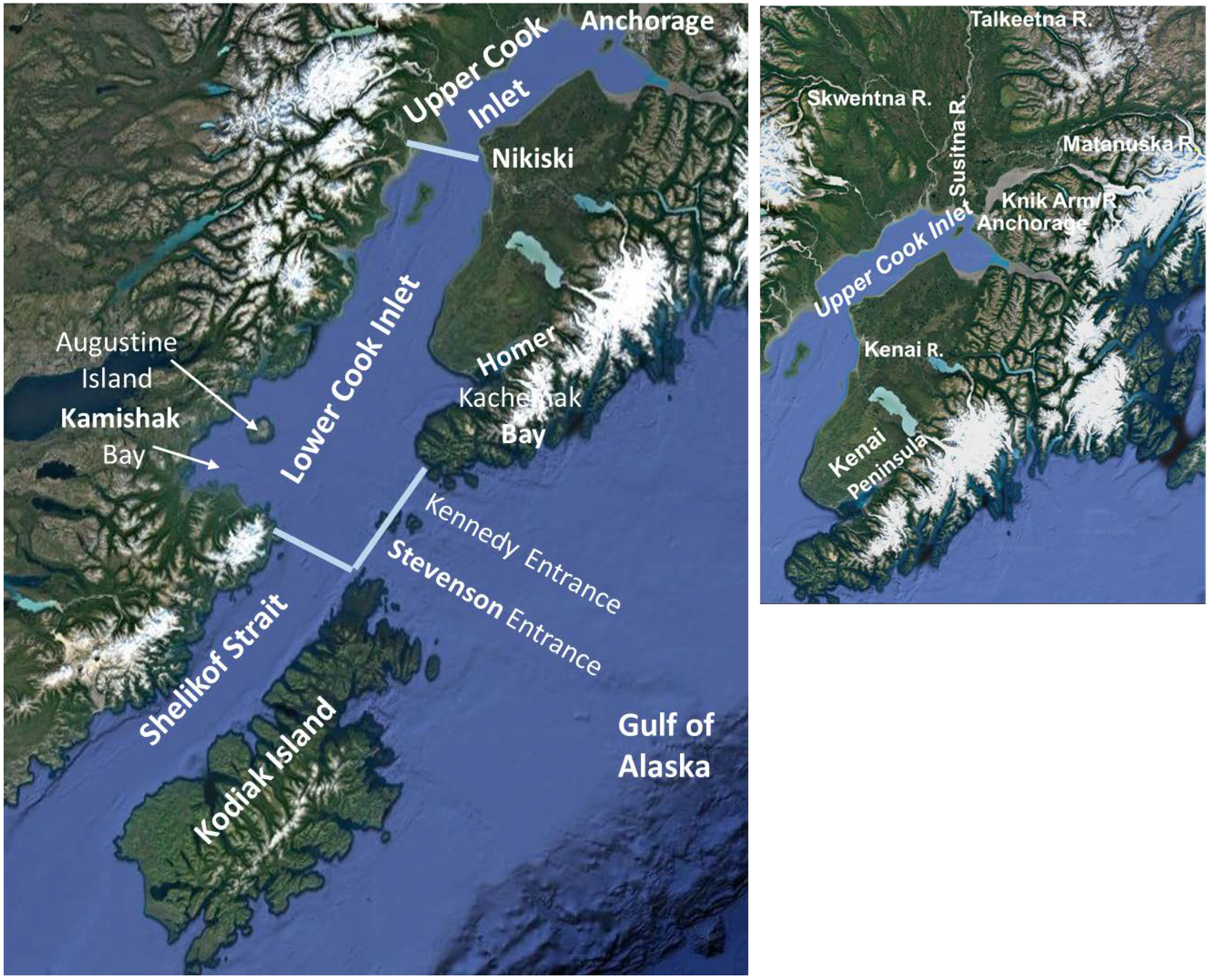
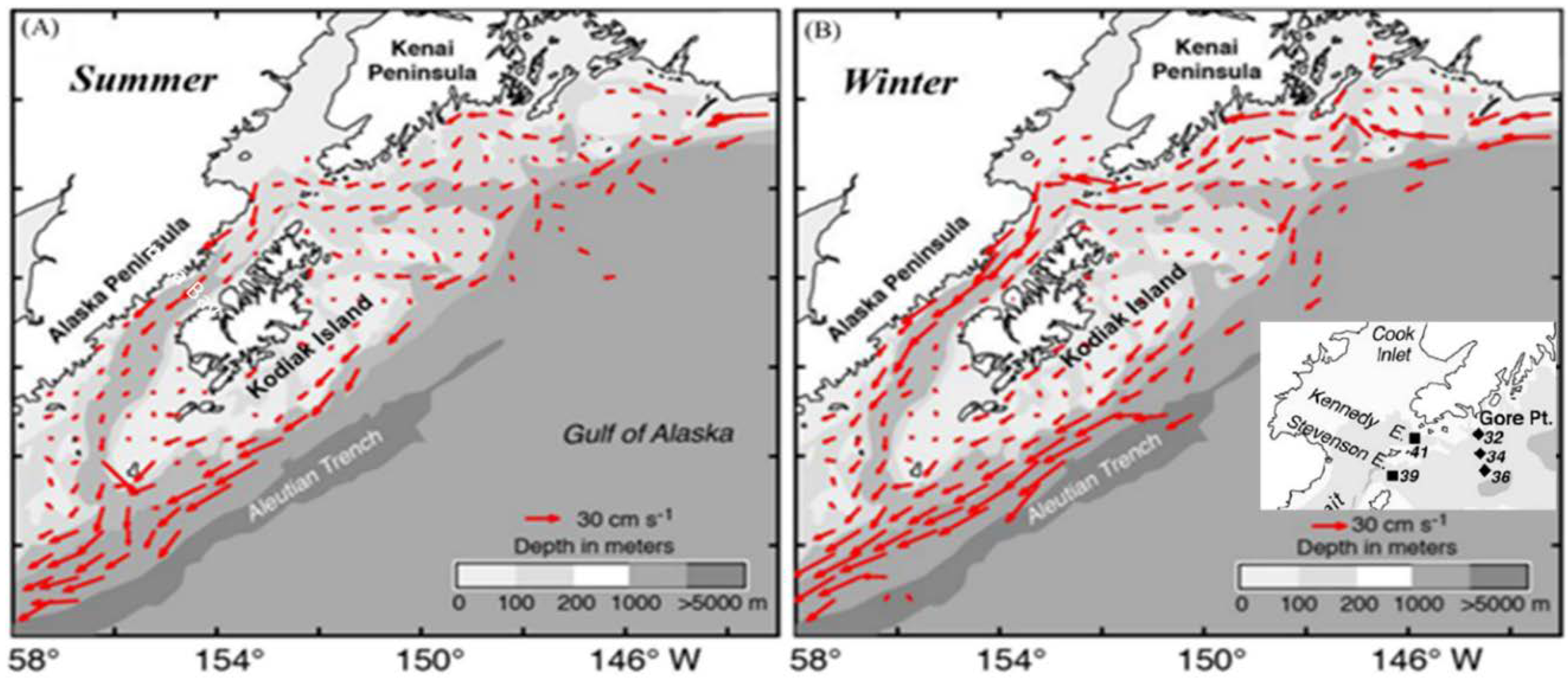
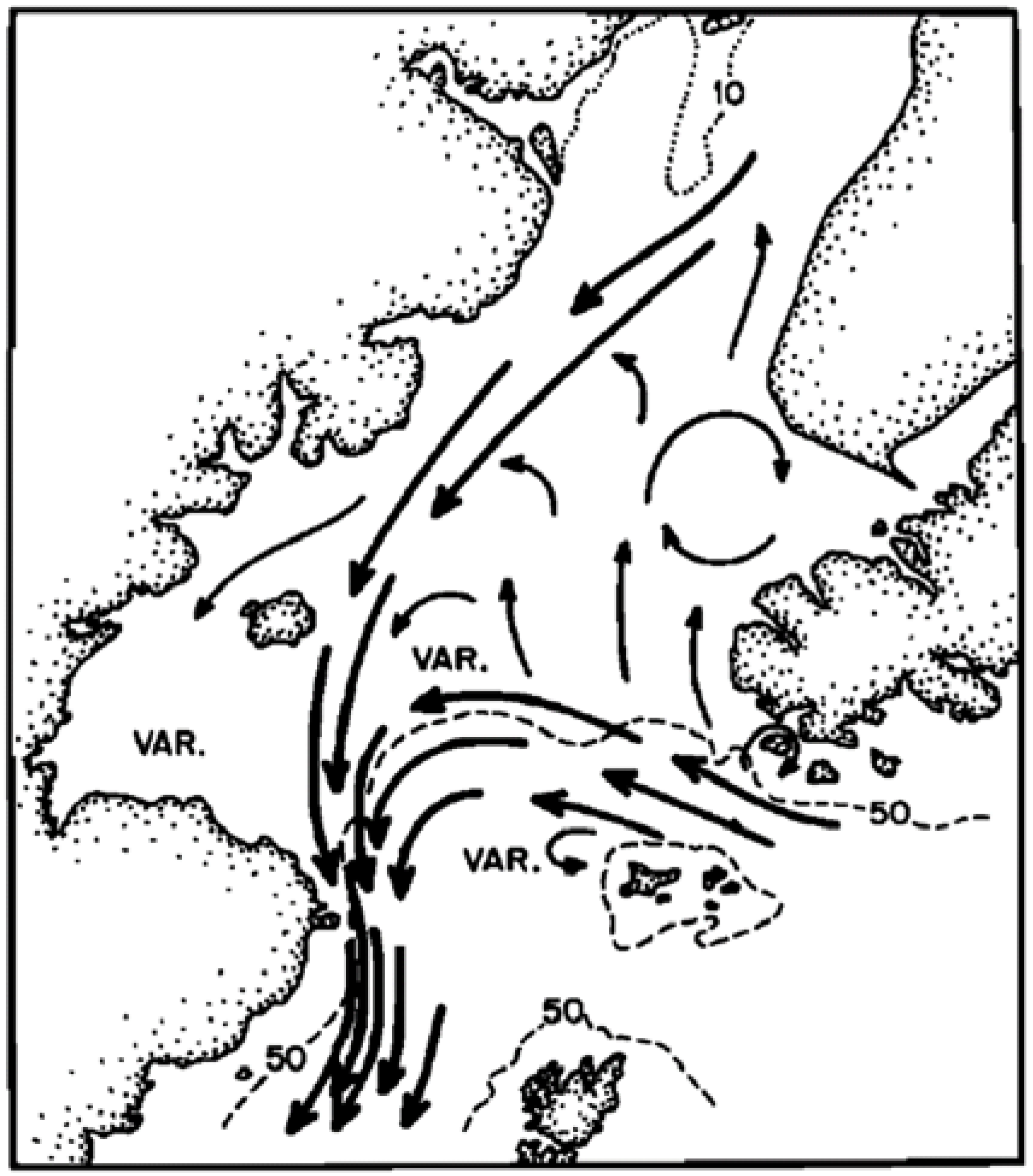
1.2. Oceanographic and Meteorological Forcing Regime in Lower Cook Inlet

The oceanographic forcing regime in LCI is complex due to a combination of large to very large tides and large seasonal winds [3] as well as freshwater discharges, and the effects of large continental shelf sub-tidal currents which penetrate into LCI from the Alaskan Continental Shelf [4].

The atmospheric forcing of Cook Inlet is dominated by the highly seasonal air temperatures from sub-freezing values spanning mid-autumn to mid-spring along with the warmer air temperatures of summer. For winds, north-easterly winds which blow seaward from UCI represent the most common wind direction, along with westerly winds originating from the Alaska mainland (Figure 2). The northwesterly winds have much larger wind speeds, with peak speeds of up to 30 m s⁻¹ by comparison to the westerly winds with peak speeds of up to 20 m s⁻¹.

The tides in Cook Inlet are very large, representing the third largest tides in North America [6] after the Bay of Fundy and Ungava Bay in Canada. The very large tides result from a resonance due to the natural oscillation period of Cook Inlet is close to the astronomical period of the semi-diurnal tides [2]. Tides enter LCI through both Kennedy and Stevenson Entrances, as well as from the south end of Shelikof Strait. Tides in Cook Inlet are mixed, mainly semidiurnal (two high and two low waters per lunar day) with tidal heights increasing northeastward (Figure 3). The mean diurnal tidal range varies from roughly 6 m at Homer to about 9.5 m at Anchorage [7]. The associated tidal currents are considerably larger in UCI and in the northward extension of LCI.

Tidal currents represent the majority of the total kinetic energy within Cook Inlet. However, buoyancy-driven subtidal currents also play an important role on the net circulation [4]. The most important subtidal current affecting the LCI area is the Alaska Coastal Current (ACC), which enters Cook Inlet through the Kennedy and Stephenson entrances (Figure 4). The ACC flows along the southern coast of the Kenai Peninsula (Figure 4) and leaves Cook Inlet along its western shore to Shelikof Strait (e.g., ref. [1]). The ACC enters the LCI area, flowing westward through Kennedy Entrance. Much of this flow turns north-westward up the east side of the Inlet, with a lesser amount travelling westward across LCI. The intensity of the ACC, and the extent of its penetration into ACC is larger in winter than in summer (Figure 4 [8,9]). The ACC represents a combination of the buoyancy resulting from extensive addition of freshwater and wind-driven coastal flow [8,10] over the continental shelf of the Gulf of Alaska.

Representing the effect from the ACC on the deeper waters of LCI is of first order importance to a numerical study for the LCI area [4,11]. Long-term observations of the ACC were analysed by Stabeno et al., 2016 [9] using the mooring data spanning a 30-year period (1984–2014, but not continuously) spread over four lines including Gore Point, and Kennedy and Stevenson Entrances. Calculated transports were found to be significantly correlated with alongshore winds (

Table 1. Statistics on transport measured. The shaded area in the first column indicates the winter period. Correlations are with NARR winds, with a positive lag indicating that the winds lead the transport (adapted from Stabeno et al., 2016 [9]). The locations of the Kennedy–Stevenson and Gore Point moorings are shown in Figure 4.

Start Date	# of 6 h Points	Correlation	Lag (Days)	95% Sig. Level	Mean Transport (106 m3 s−1)
Kennedy-Stevenson—2 moorings (3 in 1991)
10 May 1991	512	0.54	0.75	0.15	0.43
10 May 2011	512	0.70	0.75	0.28	0.56
10 May 2013	512	0.38	0.75	0.16	0.21
Gore Point—3 moorings (7 in 1991)
1 June 1991	420	0.60	0.75	0.18	0.74
10 May 1994	504	0.60	0.50	0.19	0.62
13 May 2001	486	0.46	0.50	0.17	0.57
28 May 2002	432	0.44	0.75	0.18	0.39
10 May 2003	500	0.45	0.75	0.14	0.59
10 May 2004	324	0.63	0.75	0.24	0.41
10 May 2011	500	0.65	0.50	0.25	0.44
10 May 2013	504	0.41	0.50	0.15	0.89
1 October 2001	400	0.42	0.75	0.23	1.50
1 October 2002	810	0.43	0.75	0.12	1.30
1 October 2003	810	0.46	0.75	0.13	1.31
1 October 2013	360	0.45	0.75	0.15	1.39

).

Cook Inlet has large freshwater inputs due to the direct river discharges into the Inlet as well as the inflow of marine waters from the Alaskan continental shelf. Within Cook Inlet, most of the river discharge occurs into UCI, in particular from the Susitna, Knik, and Matanuska Rivers, along with the large river discharge of the Kenai River into the northern end of LCI. Of the total drainage area of about 50,000 km², UCI receives 65% of the total drainage [12] excluding that of the Kenai River. Large freshwater input occurs during the mid-spring to summer months (April–August) because of snowmelt, as well as in the fall months (typically September–October) because of rainfall [1]. The preponderance of the river discharges into UCI and the northern end of LCI, where the strong tidal currents mix the freshwater within the comparatively shallow water column, reduces vertical stratification levels in the northern portion of Cook Inlet.

Within LCI, temperature and salinity surveys indicate that the water column is vertically stratified at low to moderate levels within the upper 40–60 m. Okkonen and Howel (2003) [13] and Okkonen et al. (2009) [14] examined temperature-salinity properties of the waters inside LCI. The ACC water flowing into Cook Inlet through Kennedy Entrance has somewhat higher salinities than the receiving waters of Cook Inlet, with the vertical density stratification being generally small due to small vertical salinity gradients in the water column below the thin upper layer of modestly reduced salinities.

Fresh water discharges from UCI results in a net southwest surface flow along the western third of LCI (Figure 5). Another major feature of the subtidal circulation is the westerly ACC flow extending from Stevenson and Kennedy Entrance into LCI which subsequently turns south on the western side of LCI and exits via Shelikof Strait; this ACC westward flow also feeds a weak northward flow of colder, more saline that penetrates along the eastern side of LCI past the Kenai Peninsula (Figure 5). The sub-tidal currents are weak on the northwestern shelf of LCI in Kamishak Bay and to the east of Augustin Island. The typical near-bottom current speeds in LCI were estimated to be above about 25 cm s⁻¹, with values of about 25 cm s⁻¹ in the western portion of the southern LCI and about 50 cm s⁻¹ in the eastern portion and in Kennedy and Stevenson entrances. These near-bottom currents were dominated by tidal currents with lesser contributions from sub-tidal flows [15].

2. Analysis of Near-Bottom Ocean Current Observations

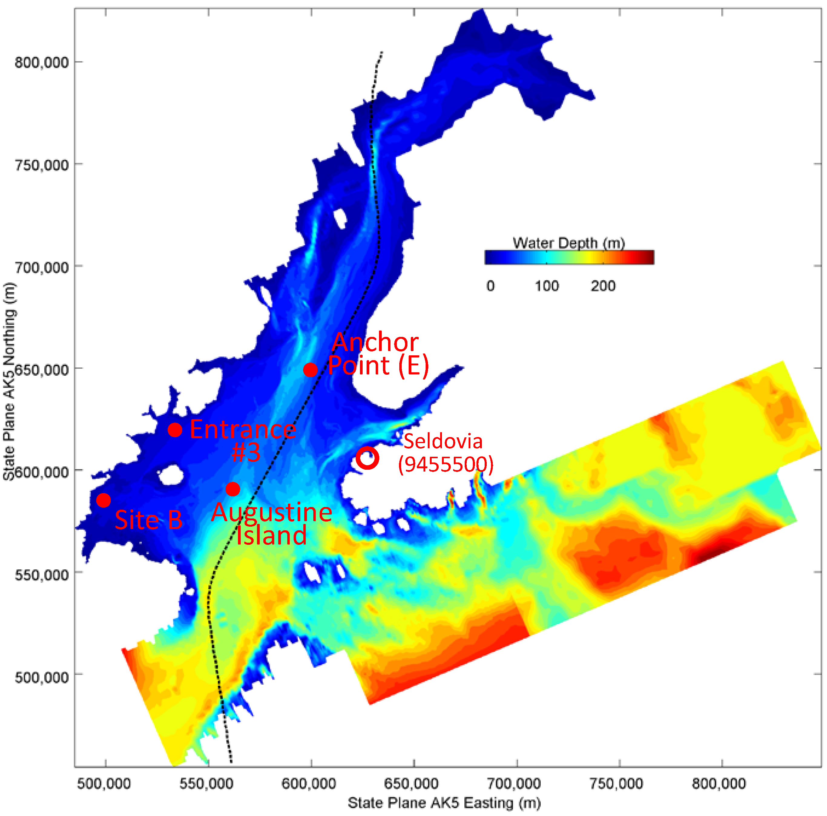
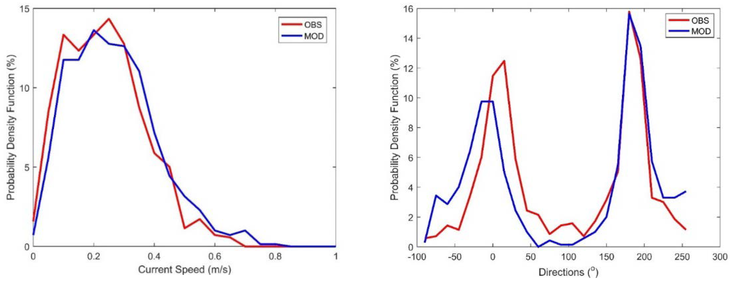
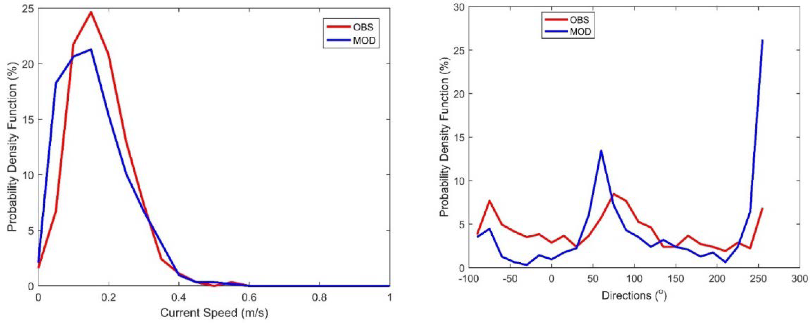
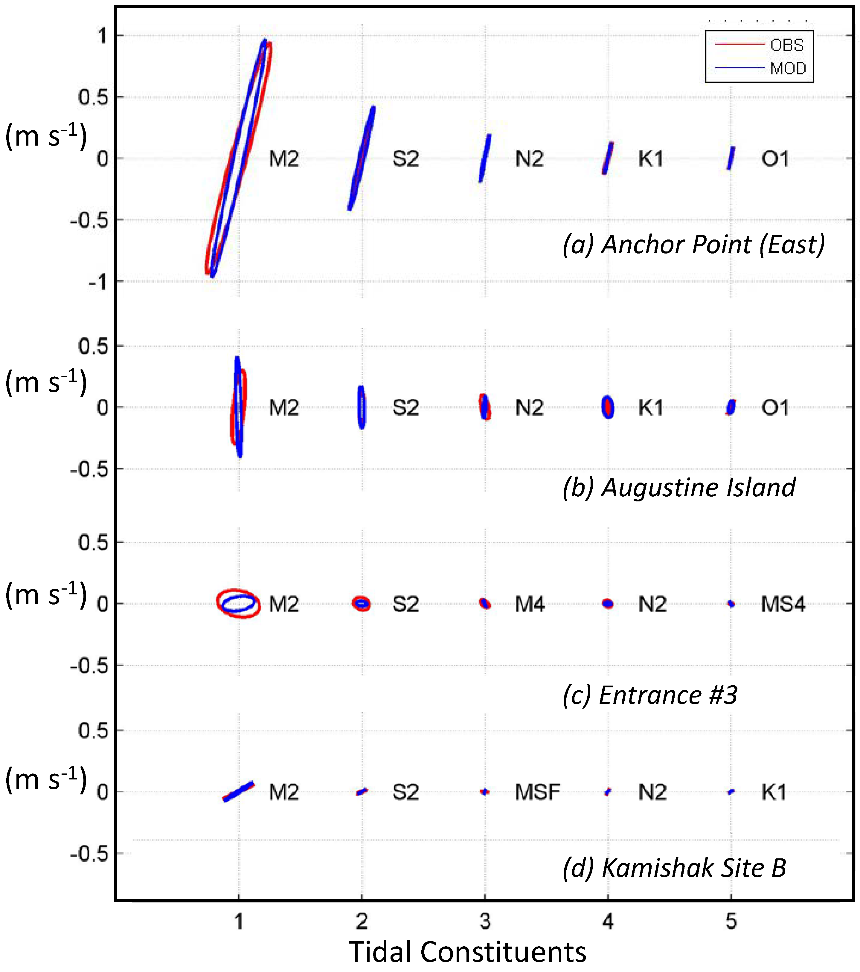
2.1. Current Meter Observations

Analyses of historical near-bottom ocean currents (Figure 6) were carried out to provide more detailed understandings of the dynamics of the near-bottom regime as well as for validation of the ocean current outputs of hydrodynamic models. Two of the data sets selected for analysis were obtained from the National Oceanic and Atmospheric Administration (NOAA) in the online Oceanographic Data Access and Processing System [16]. These measurements were made with Acoustic Doppler Current Profiler (ADCP) instruments and are typically operated for periods of one month, mostly in the summer months. The one-month duration of the measurements provides only limited value for estimation of extreme value prediction using statistical methods. Additionally, the instruments logging the current speeds were mounted on a subsea mooring facing upward at elevations several metres above the seabed, so corrections to the current speeds to a common near-bottom current elevation of 1 m, are required (see

Table 2. Analysed current meter data sets from NOAA.

NOAA Site Name	Position	Deployment Depth (m)	Sampling Interval (Seconds)	Deepest Data— Height off Bottom (m)	Start Date/Time (UTC)	End Date/Time (UTC)	Duration (Days)
Anchor Point (East)	59.818° N, 152.156° W	41.4	360	11.5	2004/08/15 16:58	2004/09/15 14:42	30.9
Augustine Island	59.302° N, 152.930° W	80.2	360	17.0	2005/07/15 02:35	2005/08/15 02:12	31.0

). The other two current meter data sets were obtained using bottom mounted ADCP’s in shallower water depths along the northwestern side of LCI: at site “Entrance #3” in the approaches to Iliamna Bay (13 October 2011, to 13 November 2012; at 15.5 m depth in 18 m total depth; [17]) and at site B in Kamishak Bay (March 2018 to March 2019, at 12 m depth in 14 m total depth; [18], operated by Terrasond), as shown in Figure 6. The current speeds are much larger at the Anchor Point (East) site than at the Augustine Island site or the two sites in western LCI.

The joint frequency distribution of the measured current speeds and directions revealed that the currents at all sites are largely bi-directional, being directed to the north-northeast on the flood tide and to the south-southwest on the ebb tide.

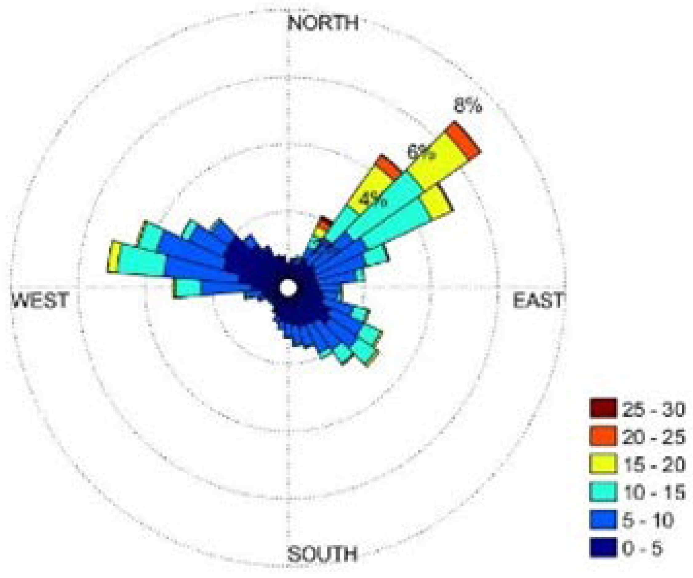
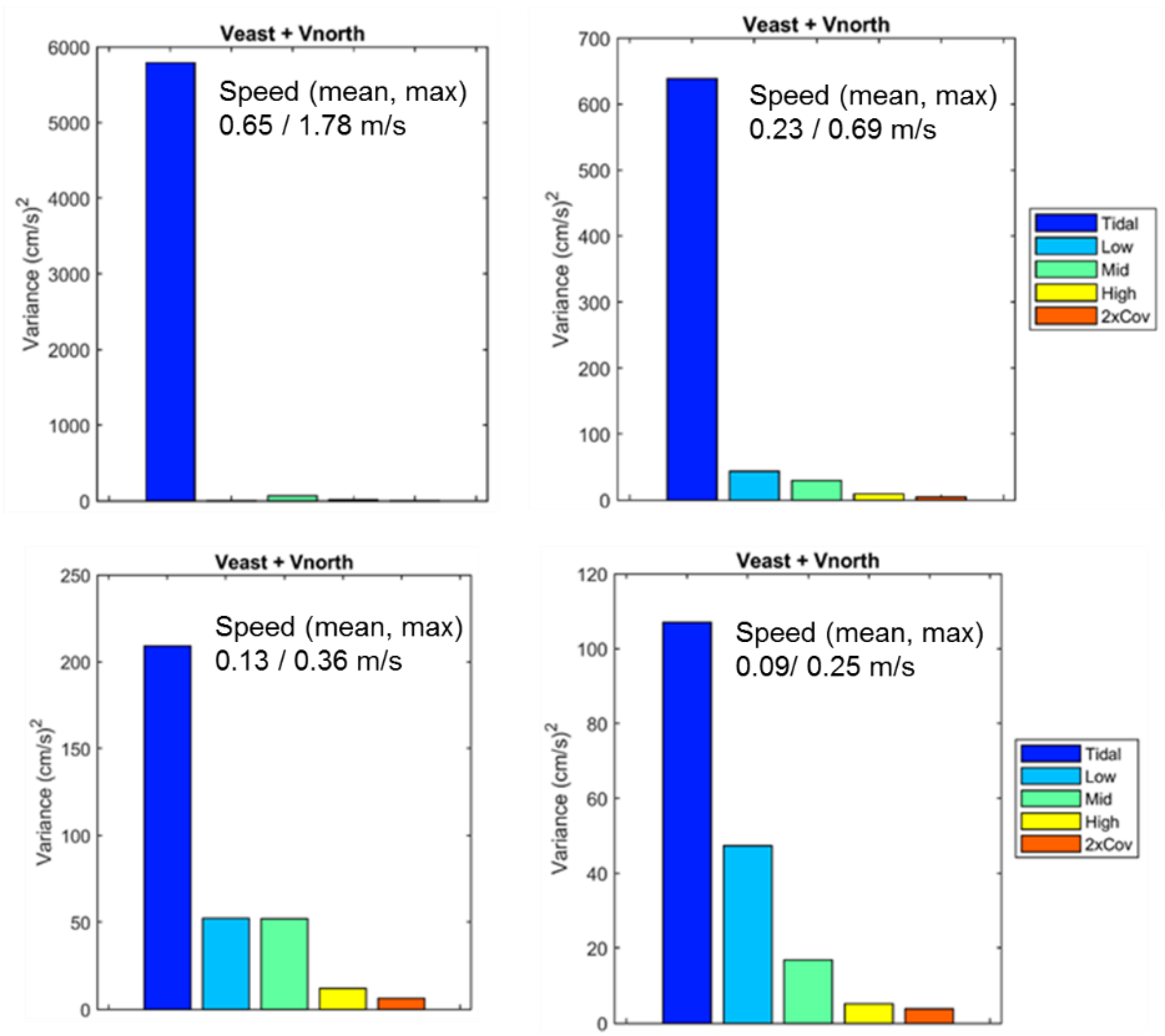
2.2. Frequency Components of Deep-Water Currents

For each current meter data set, tidal analyses and predictions were carried out using the Unified Tidal Analysis and Prediction (Utide) Matlab program [19]. The tidal predictions of the currents were subtracted from the full tidal current data set to derive the de-tided component of the currents.

The detided time series were then analysed using digital filtering methods to compute the relative magnitude of the variance for each frequency band of the currents:

• Low-pass band—filtered with a four-point Butterworth filter with a thirty-hour cut-off,
• High-pass band—filtered with a four-point Butterworth filter with a five-hour cut-off
• Mid-pass band—between 5 and 30 h—computed as the variance of the residual detided time series.

Current variance breakdown by frequency band of the currents is shown in Figure 7 for each current meter data set.

The relative proportion of variance from astronomical tides for Anchor Point (East) was extremely high at 98.5% and very high at just over 90% for Augustine Island. At the two shallow water locations (Site B and Entrance #3), the relative proportion from tidal currents were smaller, at 64% and 62%, leading to relatively larger contributions from the low- and mid-frequency bands. The dominance of tidal currents in the eastern and central portions of LCI is consistent with our understandings of the tidal regime (Figure 3) and of the sub-tidal regime (Figure 5).

3. Ocean Current Modelling

In this study, a Delft3D modeling system [20] was used. Delft3D is one of a handful of advanced deterministic (process-based) coastal ocean models, which are routinely used for this purpose [21]. The FLOW module was used to simulate the localised current speeds and directions throughout the water column using the defined bathymetry, salinity, major river discharge, wind, and tidal inputs.

Delft3D-Flow is a hydrodynamic module that uses the Navier–Stokes equations and shallow water and the Boussinesq approximation to calculate the non-steady flow and transport phenomena that occur due to wind and tidal forcing. It uses orthogonal curvilinear co-ordinates in the horizontal as the finite difference grid to solve the set of partial differential equations in combination with an appropriate set of initial and boundary conditions. The hydrostatic pressure equation is used in the vertical and the vertical velocities are calculated from the continuity equation [20].

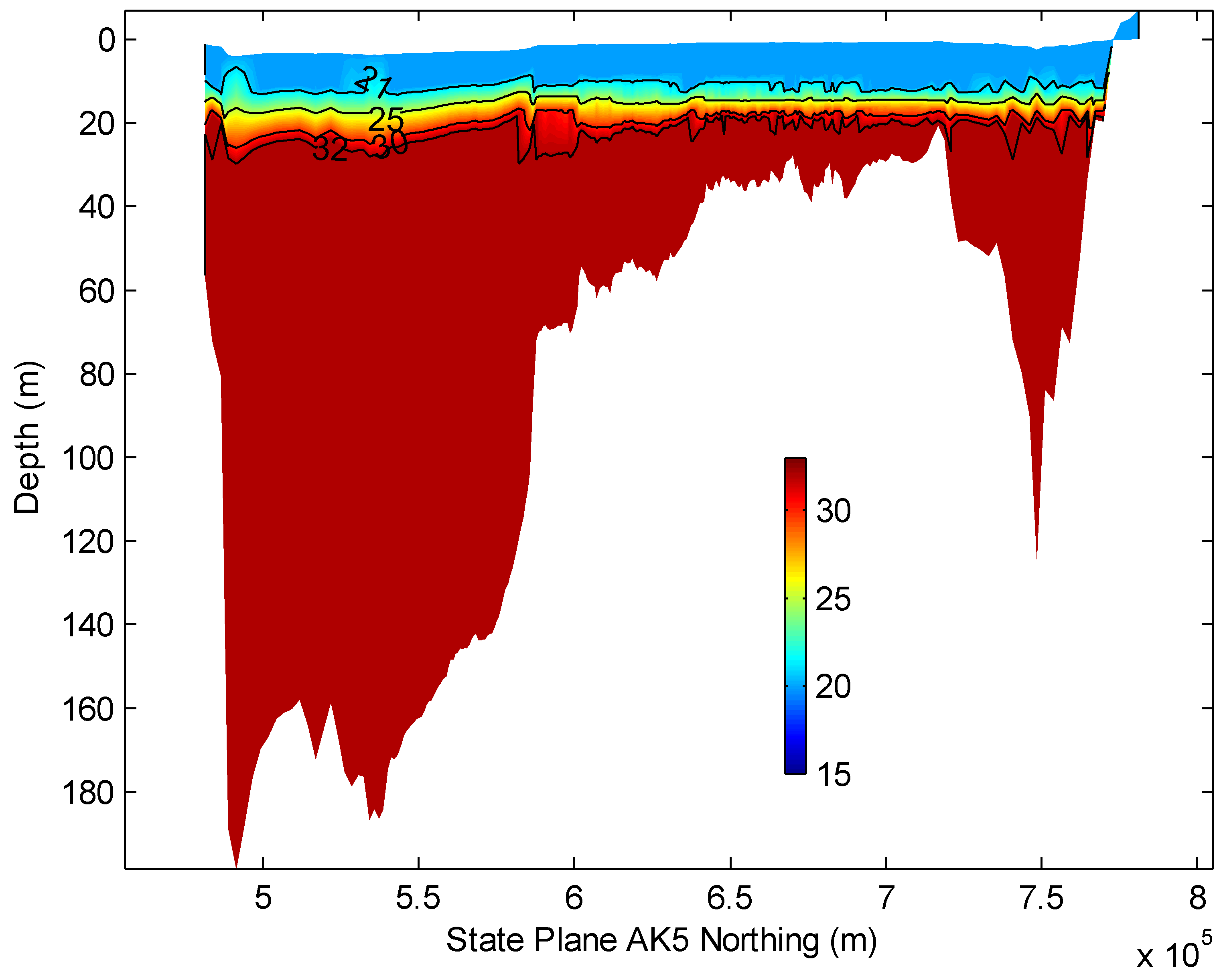
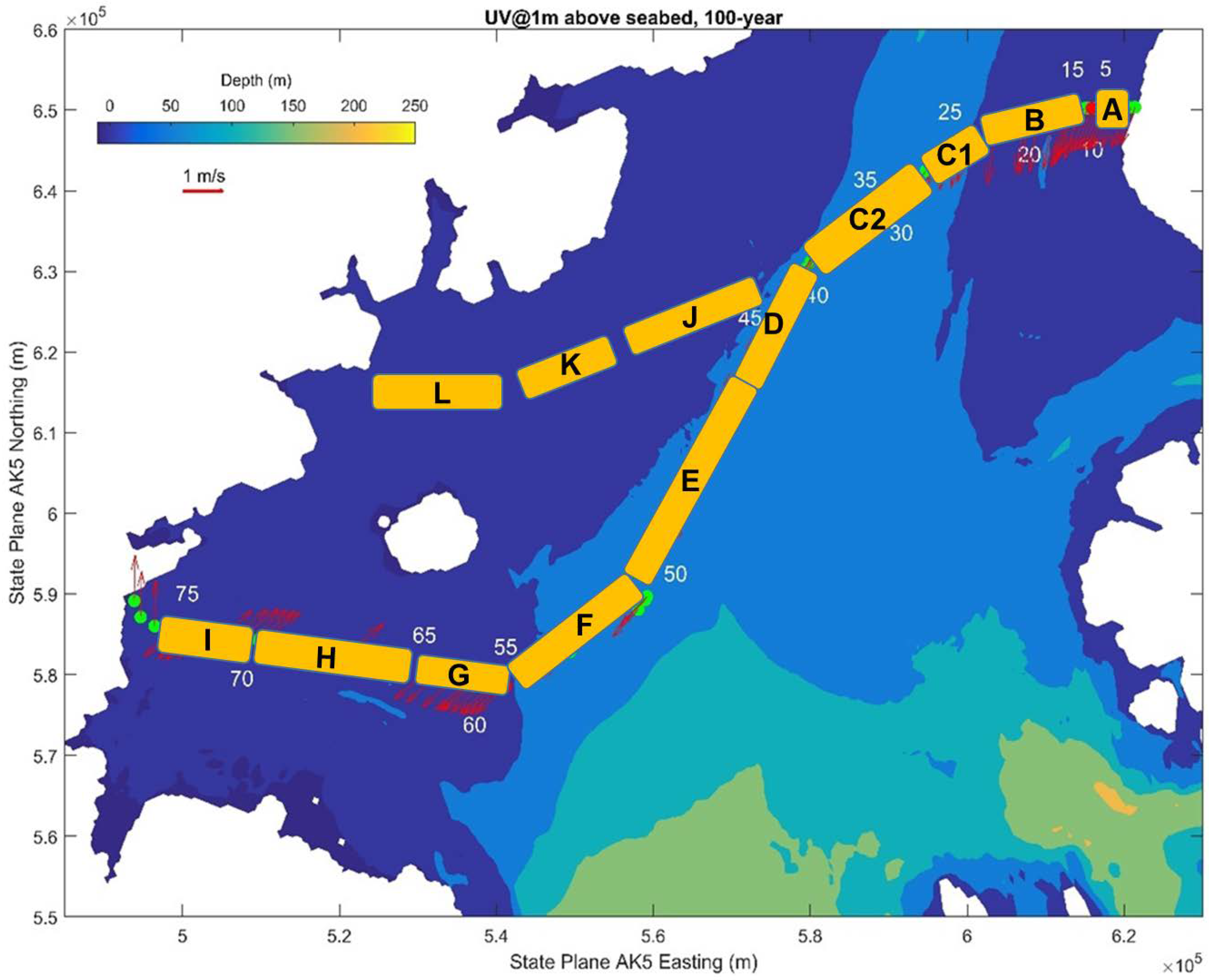
3.1. Model Domain and Development

The model domain in this study, as shown in Figure 8, includes portions of the Alaskan Continental Shelf adjoining the entrances to Cook Inlet in order to allow simulation of the effects of the ACC on LCI. The horizontal resolution in the model varies from 500 m for the LCI area to 2.5 km along the open ocean.

High resolution bathymetry for the Cook Inlet domain and Central Gulf of Alaska were obtained from the National Geophysical Data Center (NGDC) [22]. A set of fine resolution Reconnaissance Survey data available from LCI were used to augment the bathymetry. GEBCO’s 2019 gridded bathymetric data set [23] with a 15-arc-second resolution has been used to fill up uncovered areas (basically the Shelikof Strait area).

The vertical layers of the model are defined as sigma levels aligned to the seabed (which represent layers of constant fractional depth). There are 10 sigma layers with relatively higher resolution near surface and near bottom (5% of total depth), to capture both near surface stratification effects and the near bottom current variations.

At open boundaries, nine major tidal height constituents (M2, K1, S2, O1, N2, P1, SA, K2, and Q1) were specified based on NOAA water level gauge data at Station 9455090 (Seward, AK), Station 9457292 (Kodiak Island, AK), and Station 9457804 (Alitak, AK). In this study we forced a mean flow through the eastern open boundary based on the transports of ACC analysed by Stabeno et al. (2016) [9] using the mooring data spanning a 30-year period (1984–2014, but not continuously).

The external time step was set to 1.5 s to preserve stability over the simulation. The background horizontal viscosity and diffusivity coefficients were set to 0.002 and 0.01. The background vertical diffusion and viscosity were set to 10⁻⁵ m²s⁻¹ with the turbulence closure based on the κ-ε turbulence Model [20]. Bottom roughness length scale was set to 0.005 for the model bottom drag coefficient.

The model was forced by the spatially varying winds throughout the domain based on the NOAA weather stations as described above. Wind stress coefficients used the default values after model calibration.

Freshwater discharges (discussed in Section 1.2) are included in the model from major gauged rivers: the Knik, Matanuska, Susitna (and its tributaries, the Talkeetna and Skwentna Rivers) at UCI, and from the Kenai River which enters LCI more directly (Figure 1). With those river runoffs, Cook Inlet is a tidal estuary for its upper and middle parts, but southern LCI is not a classical estuary due to its large width and multiple points of exchanges with the Alaskan continental shelf. To solve the near-bottom currents, the model was integrated in a baroclinic mode. However, water temperature is not included as a variable in the model, which is a secondary factor compared with salinity on density fields. Monthly climatological data were obtained from the World Ocean Atlas (2018) [24] to initialise the model and provide the boundary conditions for salinity. The vertical structure of annual mean salinity along the inlet is shown in Figure 9.

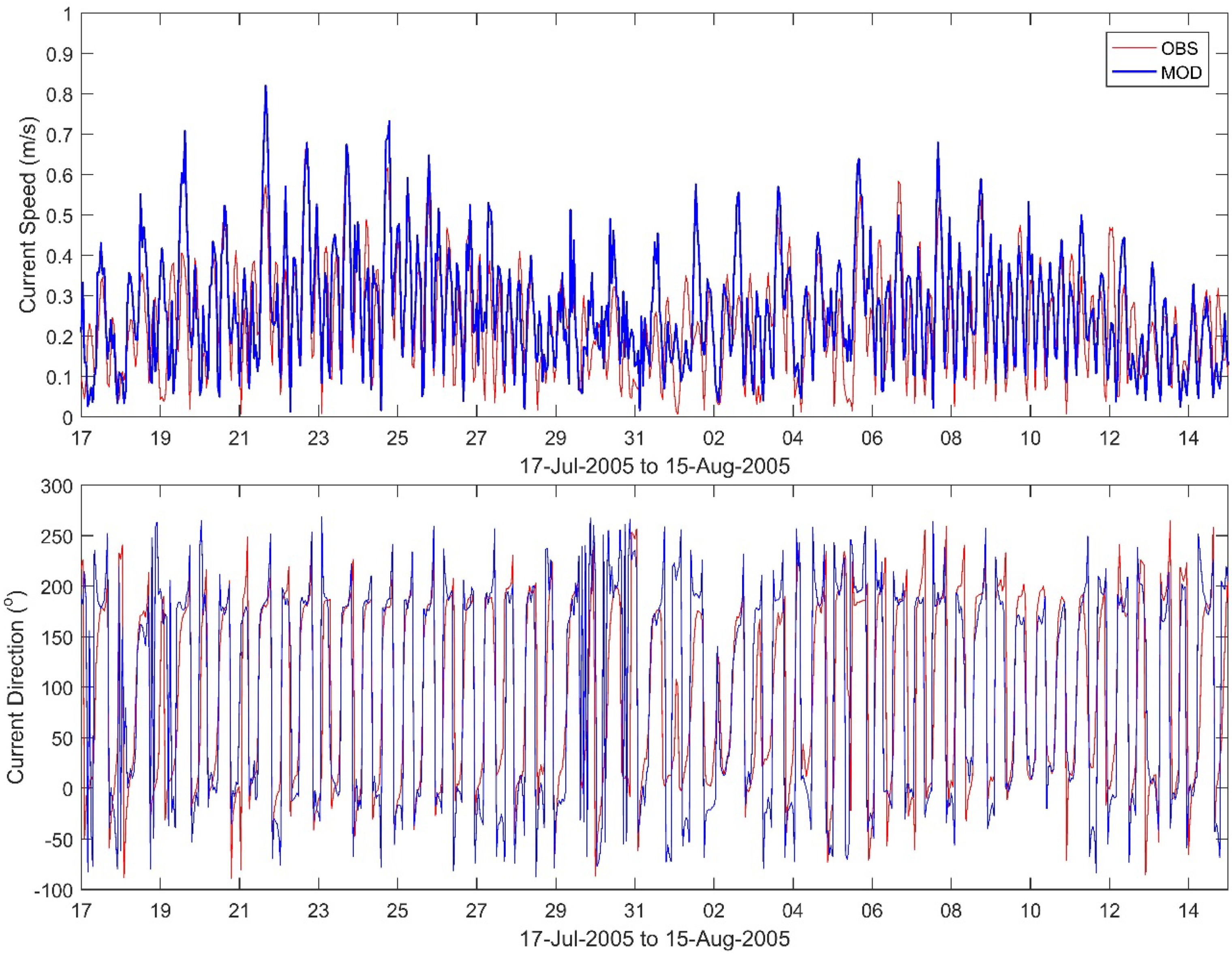
3.2. Model Calibration and Verification

The model has been calibrated and verified based on available current meter data in the study area. There are four locations of current meter data sets used for data analysis and model calibration/validation (Figure 8), which are reasonably representative of near bottom currents in southern LCI. Comparisons of the observed and modelled water levels were also made (not shown) at tidal gauge station 9455500 (Seldovia, AK; Figure 8).

The results of the verification model runs were compared to the observations at the time. The calibration run (C1) and three verification runs (V1–3) are summarised in

Table 3. Summary of calibration (C1) and verification (V1–3) runs for the Delft3D ocean circulation model.

Model Runs	Site/Location	Height above Seabed (m)	Date Start	Date End	Duration (Days)	RMSE of Current Speeds (m s−1)
C1	Anchor Point (East)	11.5	18 August 2004	14 September 2004	27	0.13
V1	Augustine Island	17.0	17 July 2005	15 August 2005	29	0.15
V2	Entrance #3	2.5	18 October 2012	13 November 2012	26	0.14
V3	Kamishak Bay Site B	1.63	1 January 2019	30 January 2019	29	0.08

.

Included in the table are a description of the location at which current information exists to compare the model results to, the height above seabed of the observations, as well as the dates and duration of the model runs. The duration of model runs ranged from 26 to 29 days in order to capture tidal currents from spring and neap tides. Model performance was assessed by root-mean-square error (RMSE) values of current speeds at current meter data sites marked in Figure 8.

Comparisons of the observed and modelled ocean currents at the measurement depths were made for each of the four calibration/verification model runs, as time series plots and as the probability density functions (PDF) of the observed and modelled currents.

Calibration run C1 was integrated for 27 days in 2004 near Anchor Point (Figure 8). The current speed and direction at the Anchor Point location compare well to the data at that time (Figure 10). Though some of the current peaks varied slightly at certain points, the progression of the current envelope through time was distinct and very similar between the two. RMSE between model results and observations was 0.13 m s⁻¹. Similarly, the current directions were almost equal throughout the full comparison period.

The probability density functions (PDF) histogram of both the current speeds and directions of the model results were compared to the historical data as well (Figure 11). Again, the current speed compared favourably, and the directions were close to exact—peaking twice at about 15 degrees and 195 degrees (180-degree opposites).

Comparisons for the verification model run V1 for NOAA Augustine Island observations are shown in Figure 12 and Figure 13. This verification event was run for 29 days in 2005 near Augustine Island (Figure 6). Though the model tended to over-estimate the peaks of the current speeds, the timing, size, and progression of the plot’s envelope closely matched those of the data (Figure 12). RMSE between model results and observations was 0.15 m s⁻¹. The modelled current direction closely matched that of the data throughout the timeline, both in timing and in value.

The PDF plot showed a similar current and percentage as its peak, and the curves closely matched (Figure 13). Directionally, the model closely matched the data at the higher of the peaks, both showing just under 16% of the current direction to be at about 180 degrees. The model did slightly miss the lower peak, predicting it to centre around 0 degrees instead of about 10–15 degrees as shown in the data.

The second model verification (V2) comparison was for site Entrance #3 in 2012 for 26 days (Figure 6). Modelled current speeds and directions at 2.5 m above seabed at Entrance to Iliamna and Iniskin Bays were comparable to the observed values, as indicated by the RMSE value of 0.14 m s⁻¹. The current speeds share a peak value (about 0.5 m s⁻¹), though the model predicted it to happen about 6 h prior to the observation time. Throughout the rest of the timeline, the model does well to predict the peak size and timing of the current speed progression.

The modelled current directions seemed variable when compared to the data; however, the PDF curve gives a better understanding (Figure 14). The model here overestimated the current flowing at 250 degrees, but decently predicted the other peak, at about 60 degrees to the model’s 75 degrees. The PDF of the current speeds show the model predicted the peak correctly to be just under 0.2 m s⁻¹, though it slightly over-estimated currents below the peak, and under-estimated above the peak.

The verification event V3 at Site B in Kamishak Bay (Figure 6) took place over 29 days in early 2019. Modelled and observed current speeds and directions were compared at 1.63 m above seabed at Site B in Kamishak Bay (not shown). Currents and directions matched well for most of the timeline, and peak currents were roughly the same size. RMSE between model results and observations is 0.08 m s⁻¹.

In plots of PDF (Figure 15), currents had the same peak, at about 0.10–0.15 m s⁻¹, with a similar curve either side of the peak. Current directions were less variable in the model than in the data, mostly peaking at about 50 and 225 degrees. The data were more spread out, and the peak directions were about 90 and 210 degrees.

For each current meter data set, tidal analyses were carried out using the Utide Matlab program [19] for both observational and modelled values. The model reproduced tidal current vectors at each site very well as to the amplitudes and directions. The tidal ellipse plots of the major tidal constituents are provided in Figure 16a Anchor Point (East), Figure 16b Augustine Island, Figure 16c Entrance #3, and Figure 16d Kamishak Bay Site B.

In general, these calibration and verification runs show that the model closely resembles the actual data for all four current meter data sets. There are some differences, but no model is perfect given the variability of the actual real-case examples. However, in all calibration/verification cases, the modelled current envelopes were closely matched to the data, and peaks were of similar size.

3.3. Scenarios for Extreme Values of Near Bottom Currents

In this section, model runs for extremal scenarios were designed and prepared. The circulation model was not operated for the full period of interest, i.e., up to 100 years, because of the limitations of computer time available. To provide appropriate and representative estimates of the return periods of the extreme currents, shorter duration model runs are made to represent a set of pre-selected one-, 10-, and 100-year extremal forcing regimes. This approach basically consists in a linear transformation of the extreme forcing to extreme responses of near bottom currents in LCI. However, for different locations, ocean responses are different, depending on whether the near bottom currents can be deterministically related to particular extremal forcing events there.

Based on the understanding of the hydrodynamics in the study area, the main dynamics affecting the near bottom currents in LCI include (1) tides, (2) local winds (especially for shallow areas), and (3) the Alaska Coastal Current inflow (ACC, as described above). Simultaneous and co-linear extreme return values of these environmental forces will create near bottom currents with a much longer return period. It is important to consider the joint occurrence of different forcing conditions (i.e., multivariate analysis).

First group of scenarios of the one-, 10-, and 100-year return periods are using model runs representative of the one-, 10-, and 100-year peak values of each forcing: ebb and flood tidal currents, wind speeds, and inflow and outflow of ACC. These are single forcing dominated mechanisms. I.e., when one forcing event is selected at extreme return events, the other two forcing conditions are at their averaged levels.

The second group of scenarios of the 10-, and 100-year return periods are for the joint probability distribution model runs. A very large spring tide (ebb and flood) occurs once every 14 days in a year (i.e., with a probability of 14/365). The largest yearly local wind has a synoptic-scale duration of 2.5 days [25,26], occurring for a probability of 2.5/365. Yearly maximum inflow and outflow of ACC, as the coastal current system driven by large scale offshore winds, also has a synoptic-scale duration of 2.5 days, i.e., with a probability of 2.5/365.

Hence the return period for the joint probability of the coincidence of an one-year maximum tide (ebb and flood) and an one-year maximum wind or ACC event is 1/[(2.5/365)*(14/365)]/365 ≈ 10 years. A similar calculation for the coincidence of an one-year maximum tide (ebb and flood) occurring with the largest 10-year value of the maximum wind or ACC results in a return period of ~100 years.

This methodology for deriving extreme near bottom current speeds in LCI was tested through comparisons with the one- and 10-year return periods derived for measured current meter results from the four verification current meter data sets. The details of the one-, 10-, and 100-year extremal forcing regimes and the model runs will be provided in the next section. Only the results of the one-, 10-, and 100-year extremal current speeds are presented as an assessment of the analysis and approach. The derived return period values based on current meter datasets were based on a Weibull distribution of the measured values with extrapolation to the one- and 10-year return periods. The comparison between the data analysis of the current meter observations and the model derived return periods at their measurement locations, provided in

Table 4. Extreme current speed model results and forecasts based on measured current speed data sets at measured height above seabed.

Site	Year	Water Depth (m)	Height above Seabed (m)	Return Period (Years)	Forecast at Measured Height above Seabed (m s−1)
					Data Analysis	Model	Difference
Anchor Point (East)	2004	41.4	11.5	1	1.78	1.69	−0.09
				10	-	1.86	-
				100	-	2.00	-
Augustine Island	2005	80.2	17.0	1	0.79	0.98	0.19
				10	-	1.25	-
				100	-	1.45	-
Entrance #3	2011–2012	18	2.5	1	0.66	0.63	−0.03
				10	0.83	0.80	−0.03
				100	-	0.98	-
Kamishak Site B	2018–2019	14	1.63	1	0.46	0.47	0.01
				10	0.53	0.58	0.05
				100	-	0.69	-

, reveals good overall agreement. The difference is normally less than 0.1 m s⁻¹, for all sites, except at Augustine Island, where the model based one-year peak current speed is 0.19 m s⁻¹ larger than the data-based value. The one-month current meter data was obtained in summer 2005 at Augustine Island site. Given the large seasonality of ocean currents to lower values during the summer period, the seasonally limited data would result in a biased prediction of the extreme event of a one-year recurrence interval, compared with the model results which include fall and winter scenarios.

3.4. Model Runs for 1 Year, 10 Year and 100 Year Return Values for Near Bottom Currents

Associated surface forcing and boundary conditions were selected and derived based on the available long-term NOAA buoy data sets as derived using extremal analysis techniques. Tidal elevations at Kodiak Island and Seldovia downloaded from NOAA were used for deriving 1-, 10- and 100-year peak tidal forcing at open boundaries. Observed wind data at the AUGA2 site from 1999–2018 were used for extremal analysis to determine peak wind events for 1-, 10-, and 100-year periods. Current speeds at the east open boundary were specified based on ACC transports. As discussed previously, the strength of ACC can be correlated to the eastward and westward wind speeds on the shelf. NOAA buoy stations 46076 provides observed wind data from 2005–2018, which were analysed to derive the 1-, 10-, and 100-year peak wind speeds, and associated inflow currents at the east open boundary into the model domain.

The details of the full set of modelled scenarios are summarised in

Table 5. Summary of case study runs for the Delft3D ocean circulation model. Each model run has a duration of 13 days.

Nominal Return Period	Model Runs	Extreme-Case Scenarios
one-year	1	Avg. Flood + 1 yr Max ACC (Single)
	2	1 yr Max Flood (Single)
	3	Avg. Ebb + 1 yr Min ACC (Single)
	4	1 yr Max Ebb (Single)
	5	Avg. Ebb + 1 yr Max Wind (Single)
10-year	1	Avg. Flood + 10 yr Max ACC (Single)
	2	Spring Flood + 1 yr Max ACC (Joint)
	3	10 yr Max Flood (Single)
	4	Avg. Ebb + 10 yr Min ACC (Single)
	5	Spring Ebb + 1 yr Min ACC (Joint)
	6	10 yr Max Ebb (Single)
	7	Avg. Ebb + 10 yr Max Wind (Single)
	8	Spring Ebb + 1 yr Max Wind (Joint)
100-year	1	Ave Flood + 100 yr Max ACC (Rescaled, single)
	2	Spring Flood + 10 yr Max ACC (Joint)
	3	100 yr Max Flood (Single)
	4	Ave Ebb + 100 yr Min ACC (Rescaled, single)
	5	Spring Ebb + 10 yr Min ACC (Joint)
	6	100 yr Max Ebb (Single)
	7	Ave Ebb + 100 yr Max Wind (Rescaled)
	8	Spring Ebb + 10 yr Max Wind (Joint)

. There are 5 model case studies for the one year return period, each run over up to two weeks in duration, for the one-year peak near bottom currents, consisting of two separate model runs for the largest flood and ebb tides representative of a one- year period; two model runs for the times of the maximum and minimum ACC values (under typical fortnightly tidal ranges); and a run representing the maximum annual northwesterly wind speed (under typical fortnightly tidal ranges).

For the 10-year return period, a similar approach was used in five model runs representative of the 10-year peak ebb and flood tidal currents, and for the 10-year maximum wind, maximum ACC, and minimum ACC conditions.

We also considered three additional model runs for very large fortnightly tidal ranges combined with one year maximum northwesterly winds, or a maximum one-year ACC or a minimum one year ACC values which are roughly equivalent to one in 10 year events. A similar approach was used in devising the eight models runs representative of extreme forcing conditions for 100-year return periods of near-bottom currents. For 100-year return periods, the values of the maximum 100-year wind speed, maximum ACC, and minimum ACC, a scaling factor was applied to the actual values, as derived through extrapolation of these peak values using a Weibull distribution of the extreme values from 10 year to 100 year return periods.

Model runs 2, 5, and 8 for the nominal 10-year and 100-year return periods for extreme near-bottom currents in LCI are based on an assumed joint probability distribution of tides, winds, and/or coastal currents.

For each nominal return period (1, 10, and 100 years), the scenario model run with the largest near-bottom current speed was selected at each model grid point of interest.

4. Summary and Conclusions

Improved understandings of the ocean circulation regime in LCI were developed, with a focus on the deeper currents near the seabed. While previous ocean circulation studies of LCI have emphasised surface and upper layer currents, there is a need for additional studies of the near-bottom current regime In this study, we analysed existing ocean current data sets for the lower part of the water column and we developed a 3D numerical hydrodynamic model for computing the near-bottom ocean currents in LCI with a wide range of various relevant forcing mechanisms.

The analysis of historical current meter data sets in LCI demonstrated that the deeper current speeds had large differences among the four locations selected in LCI. Tidal currents were very dominant in the northeast part of LCI off the Kenai Peninsula, which resulted in large values of the deeper ocean currents. In the central part of the LCI within the deep water trench, tidal currents were also important but not as completely dominant, and the total speeds were reduced in value. For the two longer duration historical current meter data located inshore on the western shelf of LCI, sub-tidal currents were found to be relatively more important, although still smaller than the contributions from the reduced amplitude of the tidal currents, resulting in substantially reduced total deep water current magnitudes.

Following extensive model calibration and validation, the numerical model was run for many cases, of up to two weeks duration, which were representative of extreme near-bottom current forcing regimes which are representative of possible return periods of 1 year, 10 years, and 100 years. From these model runs, a compilation of the model results was made, at a selected set of model grid points, for the largest values realised for each of the three return periods.

The computed 1-, 10-, and 100-year near bottom current speeds at one meter above the seabed are compiled in

Table 6. Return period values of near-bottom currents (one meter above seabed) for selected segments of the seabed (shown in Figure 17). The “Regime” values correspond to the categories in Table 5.

Segment ID	Area	Length (km)	Water Depths (m)	1 Yr. Btm. Speeds	1 Yr. Regime	10 Yr. Btm. Speeds	10 Yr. Regime	100 Yr. Btm. Speeds	100 Yr. Regime	Seq.1	Seq.L	KP-1	KP-L	KP-Mid	x (m)	y (m)	x-Adj (m)	y-Adj (m)	Lat-Mid	Lon-Mid
A	Inshore Kenai Peninsula	4	9–20	0.70–0.77	4	0.93–1.01	8	1.05–1.12	5	2	7	2	7	3	618,637.8	650,320.3	562,001.5	6,627,381.3	59.7796	−151.8957
B	Offshore Kenai Peninsula	13.5	33–44	0.99- 1.10	4	1.27–1.35	5,8	1.44–1.52	5	16	22	8.5	22	14	607,685.1	649,591.4	551,048.8	6,626,652.5
C1	Deep Trench to NE Cook Inlet-1	9	51–74	0.63–0.69	4	0.75–0.86	5	0.84–1.82	5			22	31
C2	Deep Trench to NE Cook Inlet-2	15.5	70–81	0.67–0.91	4	0.79–1.05	5	0.86–1.12	5	29	39	31	46.5	40	586,073.1	636,137.4
D	SW - NE Transect-W side (part 1)	17	53–60	0.85–0.88	4	0.80–1.03	5	0.96–1.09	5	41	44	47	62	51	578,164.0	628,917.3
E	SW - NE Transect-W side (part 2)	30.5	57–68	0.60–0.65	3,1	0.79–0.80	4	0.93–0.98	4	47	50	64.5	95	77.5	566,283.9	605,411.4	509,647.5	6,582,472.5	59.3808	−152.8302
F	Offshore Augustine Island	18	48–67	0.63–0.69	1	0.81–0.82	4	0.95–1.01	5	54	54	98	116	107	549,369.0	582,873.0	492,732.7	6,559,934.1	59.1785	−153.1272
G	Shelf W. of Augustine I.-Offshore	11.5	37–47	0.62–0.66	1	0.79–0.86	4,2	0.98–1.05	5	55	65	116	127.5	121	536,489.2	579,046.0
H	Shelf W. of Augustine I.-Middle	20	25–36	0.62–0.97	1	0.79–1.24	2	0.98–1.36	5	66	66	127.5	147.5	137.5	520,307	582,173
I	Shelf W. of Augustine I.-Inshore	13	12–24	0.70- 0.82	1,5	0.93–1.02	2,5	1.00–1.20	2,5	67	76	147.5	160.5	151	507,075.2	584,751.5	450,438.9	6,561,812.5
													13
J	Shelf E of Augustine I.-Offshore	18	38–47	0.69–0.73	3	0.91–0.94	4	1.05–1.12	4			57	75	66	564,177.94	623,383.5
K	Shelf E of Augustine I.-Middle	11	28–35	0.73–0.75	1	0.98–1.03	4	1.19–1.24	4			79	90	84.5	547,033	616,433.5
L	Shelf E of Augustine I.-Inshore	15	12–27	0.70–0.73	1	0.78–0.84	4	0.93–1.04	4			93.5	109	101	531,103	613,062.75	474,466.7	6,590,123.8
1	Anchor Point (East) CM	n/a	41	0.72	4	0.93	5	1.00	5								547,334	6,631,444	59.818	−152.156
2	Augustine Island CM	n/a	80	0.46	3	0.55	4	0.68	4								503,986	6,573,683	59.302	−152.93
3	Entrance #3 CM	n/a	18	0.62	5	0.73	5	0.83	5								477,972	6,604,703	59.58	−153.39
4	Kamishak Bay Site B CM	n/a	14	0.47	1	0.58	4	0.69	4								440,097	6,567,248	59.24	−154.05
	Law of the Wall computations									Scal.Factor							−3714.8	4791.5
1	Anchor Point (East) CM	n/a	41	1.22	4	1.34	5	1.44	5	0.72				S.End-E	559,334.0	589,906.7	502,697.7	6,566,967.8
2	Augustine Island CM	n/a	80	0.80	3	1.03	4	1.19	4	0.82				W.End-I	497,641.7	585,705.8	441,005.3	6,562,766.8
3	Entrance #3 CM	n/a	18	0.59	5	0.74	5	0.91	5	0.93
4	Kamishak Bay Site B CM	n/a	14	0.45	1	0.56	4	0.66	4	0.96

at selected segments of the seabed in LCI (shown in Figure 17). Speed values are the maximum within a 1 km distance width. These selected segments are representative for a sub-area limited to water depths of less than 90 m in LCI. The area of interest spans the Kenai Peninsula to the western coastline of LCI (from Kamishak Bay to Iliamna and Inisken Bays). These locations did not include the deep entrance of LCI (where reduced wind related near-bottom currents are expected).

The largest bottom current speeds occurred in the northeastern part of LCI to the east of the deep trench extending northwest to Central Cook Inlet extending into the deeper waters off the Kenai Peninsula (area segment B). Here, the near-bottom currents reached speeds of up to 1.1 m s⁻¹ (1-year) and up to 1.52 m s⁻¹ (100-year return period). The near-bottom current speeds were also generally high on the inner part of the Kenai Peninsula shelf (segment A) and in the northern portions of the deep trench (area segments C1, C2, and D). In these subareas A to D, the oceanographic bottom current regimes for long return periods were dominated by strong ebb tidal currents (maximum 1-year ebb tide for the one-year return period and spring tidal ebb currents combined with the minimum ACC values or maximum winds for the 10-year and 100-year return periods).

Further to the southwest in the deeper central waters of LCI, along the western side of the deeper waters off the shallower western shelf and on the outer part of the western shelf (subareas E and F), the near-bottom current speeds were generally reduced to values of 0.60–0.69 at one-year return periods and 0.93–1.01 m s⁻¹ at 100-year return periods. Here, the oceanographic regime was associated with large modes of the ACC combined with less extreme tidal currents.

In the waters of the western shelf around Augustine Island (areas F–L), the near-bottom currents had generally reduced levels. To the west of Augustine Island, at the mid-shelf (segment H), near-bottom current speeds were somewhat larger at 0.62–0.97 m s⁻¹ (one year period) and 0.98–1.36 m s⁻¹ (100-year return period). However, for most of the area segments on the shelf (segments, G, I, J, K, and L) the bottom current speeds were more moderate in the range of 0.62–0.83 m s⁻¹ (one year return period) and 0.93–1.24 m s⁻¹ (100-year return period). Over this broad shelf area, the wind-forced currents combined with average or spring tides combined with the ACC currents forced by remote winds, dominate over maximum tidal currents.

Within LCI, the extremal values for near bottom currents arise from two different types of forcing regimes. In its northeastern portion, tidal currents dominate in the generation of large bottom current speeds for long return periods. In contrast, for the western shelf portion of LCI as well as the current in the deep trench just off this western shelf, remote wind forcing over the Alaskan continental shelf, which generates Alaska Coastal Current (ACC), is generally most important although local LCI winds are occasionally dominant in a few subareas. The effects of the ACC current, which penetrates into LCI, when combined with more typical tidal currents, is generally most important in the western LCI in determining the longer return periods of near-bottom currents. Within these two large scale forcing regimes, the near-bottom current speeds also exhibit considerable variability, of the order of ±15–20%, over spatial scales of a few kilometres to a few tens of kilometres.

In this study, an approach was developed and demonstrated to deriving very long return period values for extreme near-bottom currents. This approach makes use of 21 individual 3D hydrodynamic model runs, which are based on multiple scenarios representing various different important forcing mechanisms in categories for 1-year, 10-year, and 100-year return periods. The forcing mechanism scenarios for LCI were selected based on review of previous oceanographic studies, and the analysis of historical deep water ocean current observations. The developed approach to deriving extreme value near-bottom currents is more computationally efficient than in conducting a 3D hydrodynamic model run which spans many years.

References

1. Muench, R.D.; Mofjeld, H.O.; Charnell, R.L. Oceanographic conditions in lower Cook Inlet, spring and summer 1973. J. Geophys. Res. 1978, 83, 5090–5098. [Google Scholar] [CrossRef]
2. Johnson, M.A. Subtidal surface circulation in lower Cook Inlet and Kachemak Bay, Alaska. Reg. Stud. Mar. Sci. 2021, 41, 101609. [Google Scholar] [CrossRef]
3. Johnson, M.A. Water and Ice Dynamics in Cook Inlet; Coastal Marine Institute, University of Alaska Fairbanks: Fairbanks, AK, USA, 2008. [Google Scholar]
4. Danielson, S.L.; Hedstrom, K.S.; Curchitser, E. Cook Inlet Model Calculations, Final Report to Bureau of Ocean Energy Management, M14AC00014, OCS Study, 2016, BOEM 2015-050; University of Alaska Fairbanks: Fairbanks, AK, USA; 149p.
5. National Data Buoy Center, NOAA. Available online: https://www.ndbc.noaa.gov/ (accessed on 1 June 2019).
6. Wang, T.; Yang, Z. A Tidal Hydrodynamic Model for Cook Inlet, Alaska, to Support Tidal Energy Resource Characterization. J. Mar. Sci. Eng. 2020, 8, 254. [Google Scholar] [CrossRef]
7. Moore, S.E.; Shelden, K.E.W.; Litzky, L.K.; Mahoney, B.A.; Beluga, D.J.R. Delphinapterus leucas, Habitat Associations in Cook Inlet, Alaska. Mar. Fish. Rev. 2000, 62, 60–80. [Google Scholar]
8. Stabeno, P.J.; Reed, R.K.; Schumacher, J.D. The Alaska Coastal Current: Continuity of transport and forcing. J. Geophys. Res. 1995, 100, 2477–2485. [Google Scholar] [CrossRef]
9. Stabeno, P.J.; Bell, S.; Cheng, W.; Danielson, S.; Kachel, N.B.; Mordy, C.W. Long-term observations of Alaska Coastal Current in the northern Gulf of Alaska. Deep Sea Res. Part II Top. Stud. Oceanogr. 2016, 132, 24–40. [Google Scholar] [CrossRef]
10. Royer, T.C. Coastal processes in the northern north Pacific. In The Sea; Robinson, A.R., Brink, K.H., Eds.; John Wiley & Sons, Inc.: New York, NY, USA, 1998; Volume 11, pp. 395–413. [Google Scholar]
11. Schumacher, J.D. Alaska Coastal Current Influence on Lower Cook Inlet. In Proceedings of the Cook Inlet Physical Oceanography Workshop, Homer, AK, USA, 21–22 February 2005. [Google Scholar]
12. Shi, L.; Lanerolle, L.; Chen, Y.; Cao, D.; Patchen, R.; Zhang, A.; Myers, E.P. NOS Cook Inlet Operational Forecast System: Model Development and Hindcast Skill Assessment; NOAA Technical Report NOS CS 40; NOAA: Silver Spring, MD, USA, 2020. [Google Scholar]
13. Okkonen, S.R.; Howell, S.S. Measurements of Temperature, Salinity and Circulation in Cook Inlet, Alaska; OCS Study, 2003 MMS 2003-036; US Minerals Management Service: Washington, DC, USA, 2003.
14. Okkonen, S.R.; Pegau, S.; Saupe, S.M. Seasonality of Boundary Conditions for Cook Inlet, Alaska; Coastal Marine Institute, University of Alaska Fairbanks: Fairbanks, AK, USA, 2009. [Google Scholar]
15. Muench, R.D.; Schumacher, J.D.; Pearson, C.A. Circulation in the Lower Cook Inlet, Alaska; NOAA Technical Memorandum; 1981 ERL PMEL-28; NOAA: Seattle, WA, USA, 1981; p. 26. [Google Scholar]
16. NOAA Current Measurements Interface for the Study of Tides (C-MIST). Available online: https://cmist.noaa.gov/cmist/ssl/login.do (accessed on 30 June 2022).
17. Khokhlov, A.; Sultan, N.J.; Pickering, J.W.; Wood, J. Ice Measurements in Cook Inlet, Alaska with an Acoustic Doppler Profiler. In Proceedings of the IceTech Conference, Anchorage, AK, USA, 17–20 September 2012; Available online: https://www.pndengineers.com/home/showpublisheddocument/1338/636268165137230000 (accessed on 17 May 2019).
18. Pebble Partnership. Pebble Project Final Environmental Impact Statement, Chapter 3 Affected Environment, 2020. Available online: https://www.arlis.org/docs/vol1/Pebble/Final-EIS/Pebble-FEIS-ch3_sec18-22.pdf (accessed on 5 August 2022).
19. Codiga, D.L. Unified Tidal Analysis and Prediction Using the UTide Matlab Functions. Technical Report 2011-01. Graduate School of Oceanography, University of Rhode Island, Narragansett, RI. 59p. 2011. Available online: www.po.gso.uri.edu/pub/downloads/codiga/pubs/2011Codiga-UTide-Report.pdf (accessed on 1 June 2019).
20. Deltares, 2015. Software Simulation Products and Solutions. Available online: www.deltares.nl/en/software-solutions/ (accessed on 1 June 2019).
21. Amoudry, L.O.; Souza, A.J. Deterministic coastal morphological and sediment transport modeling: A review and discussion. Rev. Geophys. 2011, 49, RG2002. [Google Scholar] [CrossRef]
22. NOAA National Centers for Environmental Information (NCEI). Available online: http://www.ngdc.noaa.gov (accessed on 15 May 2019).
23. GEBCO Gridded Bathymetry Data. Available online: https://www.gebco.net/data_and_products/gridded_bathymetry_data (accessed on 15 May 2019).
24. NOAA National Center for Environmental Information, Access to World Ocean Atlas. 2018. Available online: https://www.ncei.noaa.gov/access/world-ocean-atlas-2018/ (accessed on 1 June 2019).
25. Taylor, S.V. Northerly Surface Wind Events over the Eastern North Pacific Ocean: Spatial Distribution, Seasonality, Atmospheric Circulation, and Forcing; University of California: San Diego, CA, USA, 2006. [Google Scholar]
26. Feser, F.; Krueger, O.; Woth, K.; van Garderen, L. North Atlantic winter storm activity in modern reanalyses and pressure-based observations. J. Clim. 2021, 34, 2411–2428. [Google Scholar] [CrossRef]
Figure 1. A map of Cook Inlet with important waterways and the connecting passages to the Gulf of Alaska. Additionally shown (inset on the right) are the major rivers in the upper parts of Cook Inlet.
Jmse 10 01287 g001
Figure 2. Wind Rose for the Augustine Island National Oceanic and Atmospheric Administration (NOAA) weather station located in LCI, from 1999–2018 [5]. Wind speeds are in m s−1.
Jmse 10 01287 g002
Figure 3. Two-dimensional distributions of tidal amplitude inside Cook Inlet for the largest semi-diurnal (M2) shown in panel (a) and diurnal (K1) shown in panel (b) tidal constituents [6].
Jmse 10 01287 g003
Figure 4. Maps of the currents at ~40 m depth showing the southwestward flowing Alaska Coastal Current and its penetration into LCI and Shelikof Strait [9] for summer (A) and winter (B). The inset in the right panel shows the locations of the Kennedy–Stevenson and Gore Point moorings.
Jmse 10 01287 g004
Figure 5. The summer circulation in Lower Cook Inlet as derived from the analyses of Muench et al. (1977) [1] based on an analysis of May–September current meter and CTD measurement program.
Jmse 10 01287 g005
Figure 6. Locations of analysed current meter data sets of two sites of extended measurements over nearly one year (shown in red) obtained off Iliamna Bay (“Entrance #3”) in 2011–2012 [17] and in Kamishak Bay (“Site B”) in 2018–2019 [18] and two one-month-long NOAA data sets [16] (shown in green).
Jmse 10 01287 g006
Figure 7. An analysis of the contributions from tidal currents as well as other frequency bands, presented for Anchor Point (East), 11.5 m height off bottom (upper left) and Augustine Island, (upper right), Entrance #3 (lower left) and Kamishak Bay Site B (lower right). Low, Mid, and High refer to filtered residuals having periodicity <5 h, 5 to 30 h, and >30 h, respectively. 2xCov is a cross-covariance term included to conserve total variance.
Jmse 10 01287 g007
Figure 8. Model domain and bathymetry (projection AK5). Sites for model calibration and verification are marked as red solid dots. Tidal gauge data in LCI are available at station 9455500 (Seldovia, AK) as marked with red hollow dots. The dashed line marks the section showing the annual mean salinity structure in Figure 9.
Jmse 10 01287 g008
Figure 9. Annual mean salinity structure in Cook Inlet along the section marked in Figure 8.
Jmse 10 01287 g009
Figure 10. Current speed (upper panel) and direction (lower panel) time series for the observed (red lines) and modelled (blue lines) values at 17 m above seabed at Augustine Island (NOAA).
Jmse 10 01287 g010
Figure 11. Histogram plot for current speeds (left panel) and directions (right panel) of the observed (red lines) and modelled (blue lines) values at 17 m above seabed at Augustine Island (NOAA).
Jmse 10 01287 g011
Figure 12. Current speed (upper panel) and direction (lower panel) time series for the observed (red lines) and modelled (blue lines) values at 17 m above seabed at Augustine Island. RMSE between model results and observations is 0.15 m s−1.
Jmse 10 01287 g012
Figure 13. Histogram plot for current speeds (left panel) and directions (right panel) of the observed (red lines) and modelled (blue lines) values at 17 m above seabed at Augustine Island.
Jmse 10 01287 g013
Figure 14. Histogram plot for current speeds (left panel) and directions (right panel) of the observed (red lines) and modelled (blue lines) values at 2.5 m above seabed at Entrance #3.
Jmse 10 01287 g014
Figure 15. Histogram plot for current speeds (left panel) and directions (right panel) of the observed (red lines) and modelled (blue lines) values at 1.63 m above seabed at Site B in Kamishak Bay.
Jmse 10 01287 g015
Figure 16. Tidal ellipses (top five tidal constituents as to the amplitudes) at calibration and verification sites marked in Figure 6.
Jmse 10 01287 g016
Figure 17. Locations of segments (A–L) and sites for model calibration and verification (1–4) for which return periods of bottom currents were computed.
Jmse 10 01287 g017