
Spot Charter Rate Forecast for Liquefied Natural Gas Carriers


Abstract
:1. Introduction
2. Materials and Methods
2.1. LNG Data
2.2. Methodology
2.2.1. Variables Selection
2.2.2. Data Regression

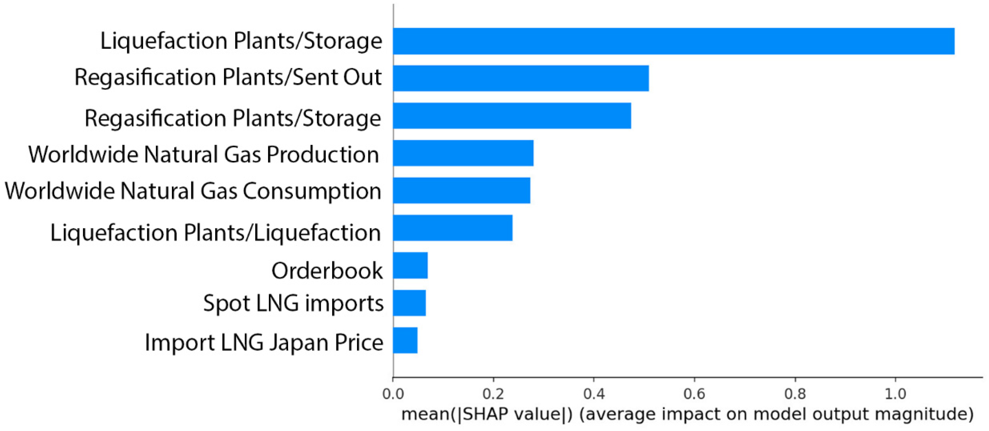
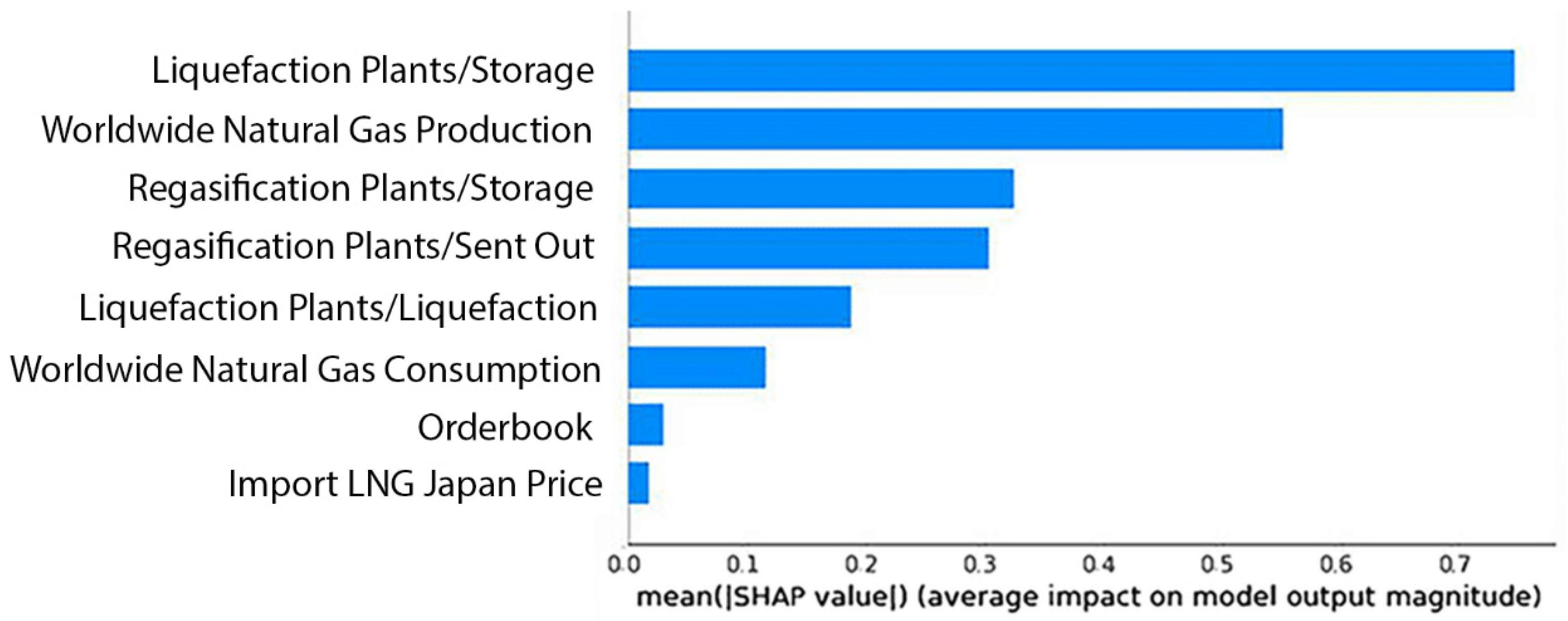
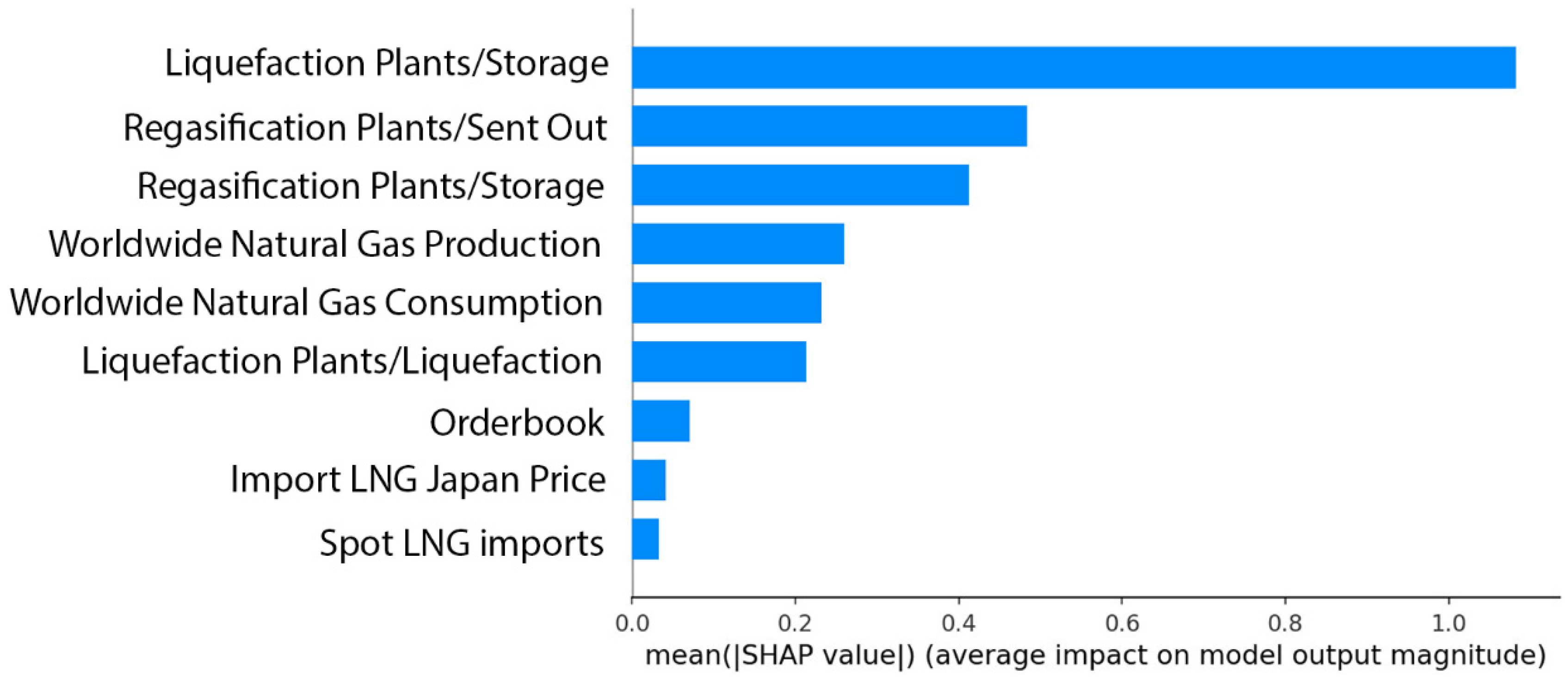
2.2.3. Post Hoc Explainability
3. Results
3.1. Evaluation Methodology
3.2. Results
4. Discussion
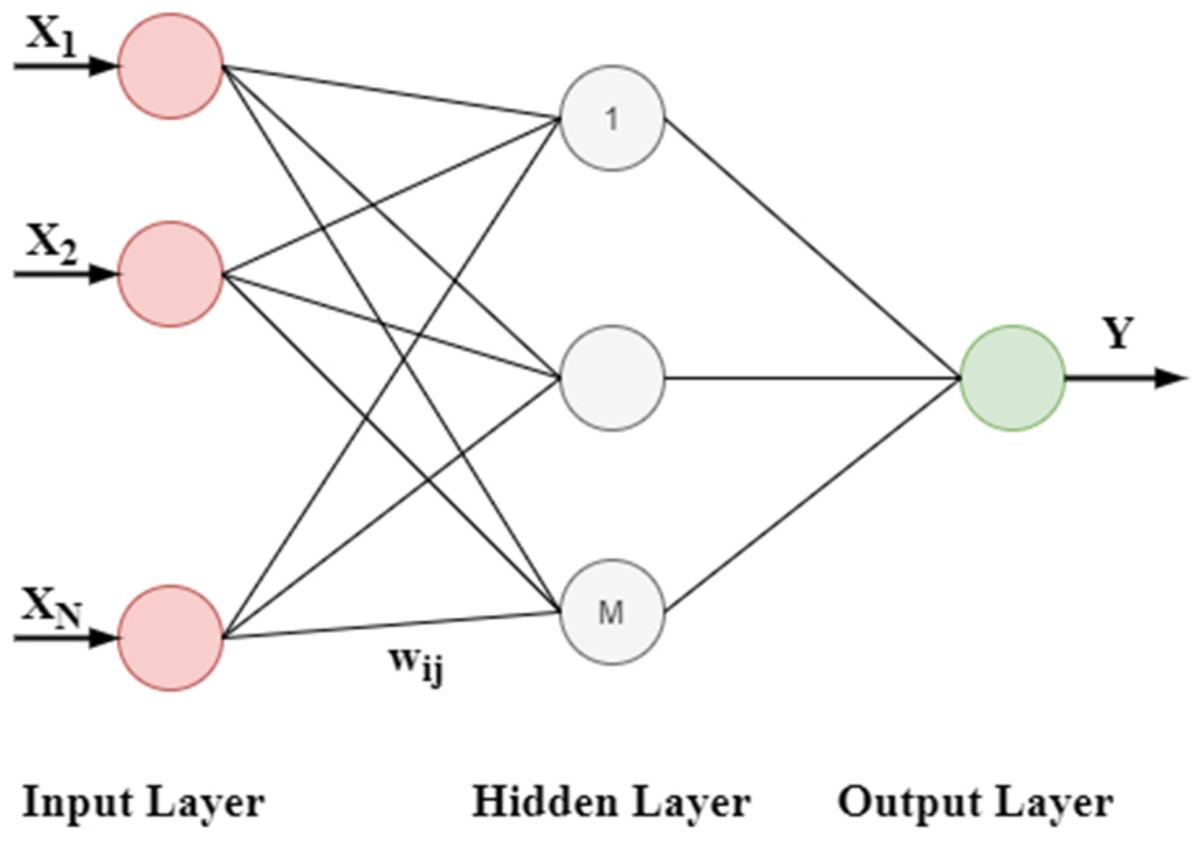
- Multilayer perceptron (MLP)
- Generalized feedforward (GFFN)
- Modular (programming)
- Jordan/Elman
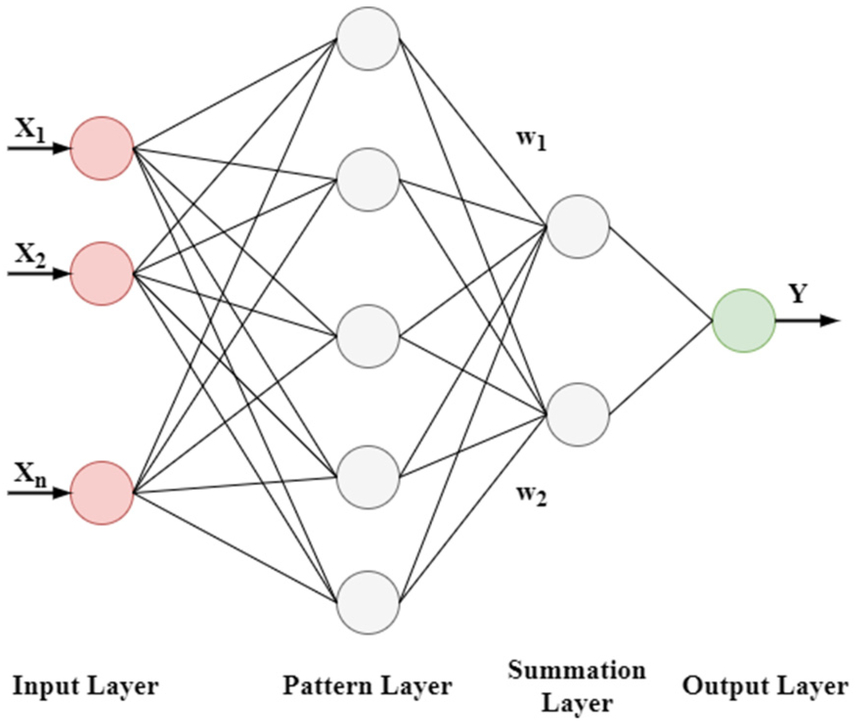
- General regression neural network (GRNN)
- Self-organizing map (SOM)
- Time-lag recurrent network (TLRN).
5. Conclusions
Funding
Institutional Review Board Statement
Informed Consent Statement
Data Availability Statement
Conflicts of Interest
References
- Awoyomi, A.; Patchigolla, K.; Anthony, E.J. Process and Economic Evaluation of an Onboard Capture System for LNG-Fueled CO2 Carriers. Ind. Eng. Chem. Res. 2020, 59, 6951–6960. [Google Scholar] [CrossRef]
- Chu Van, T.; Ramirez, J.; Rainey, T.; Ristovski, Z.; Brown, R.J. Global Impacts of Recent IMO Regulations on Marine Fuel Oil Refining Processes and Ship Emissions. Transp. Res. Part D Transp. Environ. 2019, 70, 123–134. [Google Scholar] [CrossRef]
- Seithe, G.J.; Bonou, A.; Giannopoulos, D.; Georgopoulou, C.A.; Founti, M. Maritime Transport in a Life Cycle Perspective: How Fuels, Vessel Types, and Operational Profiles Influence Energy Demand and Greenhouse Gas Emissions. Energies 2020, 13, 2739. [Google Scholar] [CrossRef]
- Pavlenko, N.; Comer, B.; Zhou, Y.; Clark, N.; Rutherford, D. The Climate Implications of Using LNG as a Marine Fuel; Swedish Environmental Protection Agency: Stockholm, Sweden, 2020.
- International Gas Union. World Lng Report; International Gas Union: Barcelona, Spain, 2020. [Google Scholar]
- GIIGNL—International Group of Liquefied Natural Gas Importers. GIIGNL Annual Report—The LNG Industry; GIIGNL: Elmwood Park, NJ, USA, 2020. [Google Scholar]
- International Energy Agency. Global Gas Security Review 2019; International Energy Agency: Paris, France, 2019. [Google Scholar]
- Atsalakis, G.S. Using Computational Intelligence to Forecast Carbon Prices. Appl. Soft Comput. J. 2016, 43, 107–116. [Google Scholar] [CrossRef]
- Dario, U. Forecasting Energy Market: An Artificial Neural Network Approach; Universita Ca’Foscari Venezia: Venice, Italy, 2015. [Google Scholar]
- Wu, Y.H.; Hua, J.; Chen, H.L. Economic Feasibility of an Alternative Fuel for Sustainable Short Sea Shipping: Case of Cross-Taiwan Strait Transport. In Proceedings of the World Congress on New Technologies, Madrid, Spain, 19–21 August 2018. [Google Scholar]
- Le Fevre, C.N. A Review of Demand Prospects for LNG as a Marine Fuel; Oxford Institute for Energy Studies: Oxford, UK, 2018. [Google Scholar]
- Merien-Paul, R.H.; Enshaei, H.; Jayasinghe, S.G. Guessing to Prediction-a Conceptual Framework to Predict LNG Bunker Demand Profile in Australia. In Proceedings of the IAMU AGA 17-Working Together: The Key Way to Enhance the Quality of Maritime Education, Training and Research, Hải Phòng, Vietnam, 26–29 October 2016; pp. 244–252. [Google Scholar]
- Aronietis, R.; Sys, C.; Van Hassel, E.; Vanelslander, T. Forecasting Port-Level Demand for LNG as a Ship Fuel: The Case of the Port of Antwerp. J. Shipp. Trade 2016, 1, 2. [Google Scholar] [CrossRef]
- Arnet, N.M.L. LNG Bunkering Operations: Establish Probabilistic Safety Distances for LNG Bunkering Operations. Master’s Thesis, Institutt for energi-Og Prosessteknikk, Trondheim, Norway, 2014. [Google Scholar]
- Jin, J.; Kim, J. Forecasting Natural Gas Prices Using Wavelets, Time Series, and Artificial Neural Networks. PLoS ONE 2015, 10, e0142064. [Google Scholar] [CrossRef]
- Al-Fattah, S.M.; Startzman, R.A. Predicting Natural Gas Production Using Artificial Neural Network. In Proceedings of the SPE Hydrocarbon Economics and Evaluation Symposium, Dallas, TX, USA, 2–3 April 2001. [Google Scholar]
- Su, M.; Zhang, Z.; Zhu, Y.; Zha, D. Data-Driven Natural Gas Spot Price Forecasting with Least Squares Regression Boosting Algorithm. Energies 2019, 12, 1094. [Google Scholar] [CrossRef]
- Busse, S.; Helmholz, P.; Weinmann, M. Forecasting Day Ahead Spot Price Movements of Natural Gas—An Analysis of Potential Influence Factors on Basis of a NARX Neural Network. In Proceedings of the Multikonferenz Wirtschaftsinformatik 2012—Tagungsband der MKWI 2012, Braunschweig, Germany, 21–22 March 2012. [Google Scholar]
- Hosseinipoor, S. Forecasting Natural Gas Prices in the United States Using Artificial Neural Networks. Master’s Thesis, University of Oklahoma, Norman, OK, USA, 2016. [Google Scholar]
- Akpinar, M.; Adak, M.F.; Yumusak, N. Day-Ahead Natural Gas Demand Forecasting Using Optimized ABC-Based Neural Network with Sliding Window Technique: The Case Study of Regional Basis in Turkey. Energies 2017, 10, 781. [Google Scholar] [CrossRef]
- Moraes, L.A.M.; Faria, L.F.T. A Stochastic Programming Approach to Liquified Natural Gas Planning. Pesqui. Oper. 2016, 36, 151–165. [Google Scholar] [CrossRef]
- Engelen, S.; Norouzzadeh, P.; Dullaert, W.; Rahmani, B. Multifractal Features of Spot Rates in the Liquid Petroleum Gas Shipping Market. Energy Econ. 2011, 33, 88–98. [Google Scholar] [CrossRef]
- Giannakopoulou, P.; Chountas, P. Forecasting the Spot Price of P1A Shipping Route. In Proceedings of the 2019 Big Data, Knowledge and Control Systems Engineering, BdKCSE 2019, Sofia, Bulgaria, 21–22 November 2019. [Google Scholar]
- von Spreckelsen, C.; von Mettenheim, H.J.; Breitner, M.H. Short-Term Trading Performance of Spot Freight Rates and Derivatives in the Tanker Shipping Market: Do Neural Networks Provide Suitable Results? In Communications in Computer and Information Science; Springer: Berlin/Heidelberg, Germany, 2012. [Google Scholar]
- von Spreckelsen, C.; von Mettenheim, H.-J.; Breitner, M.H. Spot and Freight Rate Futures in the Tanker Shipping Market: Short-Term Forecasting with Linear and Non-Linear Methods. In Operations Research Proceedings; Springer: Berlin/Heidelberg, Germany, 2014. [Google Scholar]
- Lyridis, D.V.; Manos, N.D.; Zacharioudakis, P.G. Modeling the Dry Bulk Shipping Market Using Macroeconomic Factors in Addition to Shipping Market Parameters via Artificial Neural Networks. Int. J. Transp. Econ. 2014, 41, 231–253. [Google Scholar]
- Yin, J.; Luo, M.; Fan, L. Dynamics and Interactions between Spot and Forward Freights in the Dry Bulk Shipping Market. Marit. Policy Manag. 2017, 44, 271–288. [Google Scholar] [CrossRef]
- Yip, T.L. Predicting the Shipping Market by Spreads of Timecharter Rates. Zesz. Nauk. Akad. Mor. W Szczec. 2018, 53, 9–16. [Google Scholar]
- Du, Q. Forecasting and Backtesting of VaR in International Dry Bulk Shipping Market under Skewed Distributions. Am. J. Ind. Bus. Manag. 2019, 9, 1168–1186. [Google Scholar] [CrossRef]
- Cao, J.; Li, Z.; Li, J. Financial Time Series Forecasting Model Based on CEEMDAN and LSTM. Phys. A: Stat. Mech. Appl. 2019, 519, 127–139. [Google Scholar] [CrossRef]
- Sagheer, A.; Kotb, M. Time Series Forecasting of Petroleum Production Using Deep LSTM Recurrent Networks. Neurocomputing 2019, 323, 203–213. [Google Scholar] [CrossRef]
- Schober, P.; Schwarte, L.A. Correlation Coefficients: Appropriate Use and Interpretation. Anesth. Analg. 2018, 126, 1763–1768. [Google Scholar] [CrossRef]
- Chen, P.Y.; Popovich, P.M. Correlation: Parametric and Nonparametric Measures. In Correlation; SAGE Publications, Inc.: Thousand Oaks, CA, USA, 2011. [Google Scholar]
- Herbrich, R.; Graepel, T.; Obermayer, K. Regression Models for Ordinal Data: A Machine Learning Approach; Fachbereich 13, Informatik. TR-99/03; Technische Universität Berlin: Berlin, Germany, 1999. [Google Scholar]
- Madsen, H. Time Series Analysis; Taylor & Francis eBooks: New York, NY, USA, 2007; ISBN 9781420059687. [Google Scholar]
- Wang, K.; Li, K.; Zhou, L.; Hu, Y.; Cheng, Z.; Liu, J.; Chen, C. Multiple Convolutional Neural Networks for Multivariate Time Series Prediction. Neurocomputing 2019, 360, 107–119. [Google Scholar] [CrossRef]
- Hassoun, M.H. Fundamentals of Artificial Neural Networks. Proc. IEEE 2005, 84, 906. [Google Scholar] [CrossRef]
- Buscema, P.M.; Massini, G.; Breda, M.; Lodwick, W.A.; Newman, F.; Asadi-Zeydabadi, M. Artificial Neural Networks. In Studies in Systems, Decision and Control; Springer: Berlin/Heidelberg, Germany, 2018. [Google Scholar]
- Laptev, N.; Yosinski, J.; Li, E.L.; Smyl, S. Time-Series Extreme Event Forecasting with Neural Networks at Uber. Comput. Sci. 2017, 34, 1–5. [Google Scholar]
- Che, Z.; Purushotham, S.; Cho, K.; Sontag, D.; Liu, Y. Recurrent Neural Networks for Multivariate Time Series with Missing Values. Sci. Rep. 2018, 8, 6085. [Google Scholar] [CrossRef] [PubMed]
- Caterini, A.L.; Chang, D.E. Recurrent Neural Networks. In SpringerBriefs in Computer Science; Springer: Berlin/Heidelberg, Germany, 2018. [Google Scholar]
- Hewamalage, H.; Bergmeir, C.; Bandara, K. Recurrent Neural Networks for Time Series Forecasting: Current Status and Future Directions. Int. J. Forecast. 2020, 37, 388–427. [Google Scholar] [CrossRef]
- Elman, J.L. Finding Structure in Time. Cogn. Sci. 1990, 14, 179–211. [Google Scholar] [CrossRef]
- Jordan, M.I. Chapter 25 Serial Order: A Parallel Distributed Processing Approach. In Advances in Psychology; Elsevier: Amsterdam, The Netherlands, 1997. [Google Scholar]
- Taud, H.; Mas, J.F. Multilayer Perceptron (MLP). In Geomatic Approaches for Modeling Land Change Scenarios; Springer: Cham, Switzerland, 2018; pp. 451–455. [Google Scholar]
- Zhou, Y.; Xia, J.; Shen, H.; Zhou, J.; Wang, Z. Extended Dissipative Learning of Time-Delay Recurrent Neural Networks. J. Frankl. Inst. 2019, 356, 8745–8769. [Google Scholar] [CrossRef]
- Dayhoff, J.; Omidvar, O. Locally Recurrent Networks: The Gamma Operator, Properties, and Extensions. In Neural Networks and Pattern Recognition; Oxford University Press: Cary, NC, USA, 1998. [Google Scholar]
- Cigizoglu, H.K. Generalized Regression Neural Network in Monthly Flow Forecasting. Civ. Eng. Environ. Syst. 2005, 22, 71–81. [Google Scholar] [CrossRef]
- Specht, D.F. A General Regression Neural Network. IEEE Trans. Neural Netw. 1991, 2, 568–576. [Google Scholar] [CrossRef]
- Firat, M.; Gungor, M. Generalized Regression Neural Networks and Feed Forward Neural Networks for Prediction of Scour Depth around Bridge Piers. Adv. Eng. Softw. 2009, 40, 731–737. [Google Scholar] [CrossRef]
- Nikoo, M.; Sadowski, Ł.; Khademi, F.; Nikoo, M. Determination of Damage in Reinforced Concrete Frames with Shear Walls Using Self-Organizing Feature Map. Appl. Comput. Intell. Soft Comput. 2017, 2017, 1–10. [Google Scholar] [CrossRef]
- Ntakolia, C.; Anagnostis, A.; Moustakidis, S.; Karcanias, N. Machine Learning Applied on the District Heating and Cooling Sector: A Review. Energy Syst. 2022, 13, 1–30. [Google Scholar] [CrossRef]
- Liu, H.; Yan, G.; Duan, Z.; Chen, C. Intelligent Modeling Strategies for Forecasting Air Quality Time Series: A Review. Appl. Soft Comput. 2021, 102, 106957. [Google Scholar] [CrossRef]
- Arulampalam, G.; Bouzerdoum, A. A Generalized Feedforward Neural Network Architecture for Classification and Regression. Neural Netw. 2003, 16, 561–568. [Google Scholar] [CrossRef]
- Ntakolia, C.; Kokkotis, C.; Moustakidis, S.; Tsaopoulos, D. Prediction of Joint Space Narrowing Progression in Knee Osteoarthritis Patients. Diagnostics 2021, 11, 285. [Google Scholar] [CrossRef] [PubMed]
- Lundberg, S.M.; Lee, S.-I. A Unified Approach to Interpreting Model Predictions. In Proceedings of the 31st International Conference on Neural Information Processing Systems, Long Beach, CA, USA, 4–9 December 2017; Volume 30. [Google Scholar]
- Ntakolia, C.; Kokkotis, C.; Karlsson, P.; Moustakidis, S. An Explainable Machine Learning Model for Material Backorder Prediction in Inventory Management. Sensors 2021, 21, 7926. [Google Scholar] [CrossRef] [PubMed]
- Kokkotis, C.; Ntakolia, C.; Moustakidis, S.; Giakas, G.; Tsaopoulos, D. Explainable Machine Learning for Knee Osteoarthritis Diagnosis Based on a Novel Fuzzy Feature Selection Methodology. Phys. Eng. Sci. Med. 2022, 45, 219–229. [Google Scholar] [CrossRef]
- Ntakolia, C.; Priftis, D.; Charakopoulou-Travlou, M.; Rannou, I.; Magklara, K.; Giannopoulou, I.; Kotsis, K.; Serdari, A.; Tsalamanios, E.; Grigoriadou, A.; et al. An Explainable Machine Learning Approach for COVID-19′s Impact on Mood States of Children and Adolescents during the First Lockdown in Greece. Healthcare 2022, 10, 149. [Google Scholar] [CrossRef] [PubMed]


| Data Source | Data Description of Time Series |
|---|---|
| Clarkson PLC Shipping Intelligence Network | LNG 145K CBM spot rate (USD/day): the desired prediction variable. It represents the price of the daily fare for an LNG tanker with a capacity of 145,000 CBM and a steam turbine vessel. LNG 160K CBM spot rate (USD/day): the price of the daily fare for an LNG tanker with a capacity of 160,000 CBM, tri-fuel diesel electric (TFDE). LNG 160K CBM 1 Year Timecharter Rate (USD/day) presents the price of the daily fare for one-year contracts for a ship with the same characteristics as above. World Seaborne LNG Trade (million tonnes) reveals the demand for LNG regarding the quantity that is traded internationally. World Seaborne LNG Trade (billion tonne-miles) represents the trade of LNG, multiplied by the distance that the commodity has traveled. Import LNG Japan Price (USD/mmbtu): the import price of LNG in Japan. |
| GIIGNL International Group of LNG Importers | Total LNG Fleet reveals the number of vessels that transport LNG. Total Shipping Capacity (m3—CBM) is related to the offer and shows the total capacity of all LNG vessels. Operational Capacity (m3—CBM) presents the total operating capacity for trading LNG. Its combination with the operating capacity shows the percentage of ships that are inactive at a specific time in the market. New Orders Placed indicate the attitude of shipowners toward the future of the LNG market. Orderbook shows reflects the capacity and the ability of shipyards to accept new orders in near future. Ships Delivered That Year presents the number of ships that the shipyards deliver in that year. Liquefaction Plants/Liquefaction (million tonnes per annum—MTPA) presents the amount of gas that is liquefied. While new liquefaction plants are being built, it shows that the market is on the rise. Liquefaction Plants/Storage (m3—CBM) directly affects the short-term purchase of LNG. The storage capacity was one of the main factors that led to the rise of the short-term market, allowing sellers to keep the quantities they produce and dispose of them whenever they consider it necessary. Regasification Plants/Storage (m3—CBM) shows the evolution of the ability to store LNG in regasification stations. Regasification Plants/Sent Out (billion cubic meters—bcm/year) refers to the annual quantities of LNG that is gasified. Spot LNG Imports (million tonnes) is linked with the quantities of LNG imported under the direct delivery regime. |
| U.S. Energy Information Administration (EIA) | Price of Liquefied U.S. Natural Gas Exports (USD/thousand cubic feet): the price of LNG exported by the USA. Henry Hub Natural Gas Spot Price (USD/million btu): Henry Hub is a gas pipeline located in Louisiana, USA. It is the pricing reference point for gas contracts traded on the New York Mercantile Exchange (NYMEX). Settlement prices are used as benchmarks for the entire North American gas market as well as for parts of the global LNG market. It is an important indicator as the price of natural gas is based on real supply and demand as a standalone commodity. WTI Oil Price (USD/barrel): West Texas Intermediate (WTI) crude oil is the basis for New York oil futures contracts. This indicator is important as it is a reference point for buyers and sellers of oil. Brent Oil Price (USD/barrel): Brent is a blend of crude oil exported from the North Sea. It is the reference point for most of the crude oil in the Atlantic basin and it is used to price two thirds of the crude oil traded internationally. |
| BP Statistical Review of World Energy | Worldwide Natural Gas Production (billion cubic meters—bcm) shows the global production of natural gas. Worldwide Natural Gas Consumption (billion cubic meters—bcm) shows the global consumption of natural gas. |
| LNG 145K CBM Spot Rate | Value (USD/Day) |
|---|---|
| 1 March 2017 | 31,681 |
| 1 May 2017 | 34,768 |
| 1 July 2017 | 37,854 |
| Value | Correlation |
|---|---|
| total positive linear correlation | |
| total negative linear correlation | |
| no linear correlation | |
| low–medium linear correlation | |
| medium linear correlation | |
| medium–high linear correlation | |
| high linear correlation |
| Neural Networks | |
|---|---|
| Name | Number of Parameters |
| Multilayer Perceptron (MLP) | 4 (Hidden Layers) |
| Generalized Feedforward (GFFN) | 4 (Hidden Layers) |
| Modular Neural Network (MNN) | 4 (Types) |
| Jordan/Elman Network | 4 (Types) |
| General Regression Neural Network (GRNN) | 4 (Hidden Layers) |
| Self-Organizing Feature Map Network (SOFM) | 4 (Hidden Layers) |
| Time-Lag Recurrent Network (TLRN) | 4 (Hidden Layers) |
| Variables for Prediction | |
| Name | Prediction Time |
| LNG 145K CBM Spot Rate | 2 months |
| LNG 145K CBM Spot Rate | 4 months |
| LNG 145K CBM Spot Rate | 6 months |
| Data allocation | |
| Name | Percentage |
| Training data | 75% |
| Testing data | 10% |
| Cross validation data | 15% |
| Number of epochs | |
| 1000 | |
| Name of Variable | LNG 145K CBM Spot Rate 2 Months | LNG 145K CBM Spot Rate 4 Months | LNG 145K CBM Spot Rate 6 Months |
|---|---|---|---|
| LNG 145K CBM Spot Rate | 0.987 | 0.964 | 0.933 |
| LNG 160K CBM Spot Rate | 0.964 | 0.929 | 0.889 |
| World Seaborne LNG Trade (Million Tonnes) | −0.676 | −0.690 | −0.699 |
| World Seaborne LNG Trade (Billion Tonne-Miles) | −0.115 | −0.172 | −0.222 |
| LNG 160K CBM 1 Year Timecharter Rate | 0.933 | 0.897 | 0.855 |
| Price of Liquefied U.S. Natural Gas Exports | 0.217 | 0.206 | 0.193 |
| Henry Hub Natural Gas Spot Price | 0.221 | 0.248 | 0.272 |
| Import LNG Japan Price | 0.789 | 0.742 | 0.700 |
| WTI Oil Price | 0.666 | 0.626 | 0.593 |
| Brent Oil Price | 0.729 | 0.683 | 0.639 |
| Total LNG Fleet | −0.915 | −0.929 | −0.935 |
| Total Shipping Capacity | −0.901 | −0.915 | −0.921 |
| Operational Capacity | −0.909 | −0.932 | −0.945 |
| New Orders Placed | 0.294 | 0.265 | 0.243 |
| Orderbook | −0.726 | −0.776 | −0.816 |
| Ships Delivered That Year | −0.934 | −0.925 | −0.906 |
| Liquefaction Plants/Liquefaction | −0.815 | −0.827 | −0.834 |
| Liquefaction Plants/Storage | −0.885 | −0.906 | −0.917 |
| Regasification Plants/Storage | −0.838 | −0.871 | −0.895 |
| Regasification Plants/Sent Out | −0.839 | −0.874 | −0.901 |
| Spot LNG Imports | −0.700 | −0.746 | −0.783 |
| Worldwide Natural Gas Production | −0.821 | −0.858 | −0.886 |
| Worldwide Natural Gas Consumption | −0.804 | −0.837 | −0.863 |
| Name of Variable | LNG 145K CBM Spot Rate 2 Months | LNG 145K CBM Spot Rate 4 Months | LNG 145K CBM Spot Rate 6 Months |
|---|---|---|---|
| World Seaborne LNG Trade (Billion Tonne-Miles) | no correlation | no correlation | low–medium correlation |
| Price of Liquefied U.S. Natural Gas Exports | low–medium correlation | low–medium correlation | no correlation |
| Henry Hub Natural Gas Spot Price | low–medium correlation | low–medium correlation | low–medium correlation |
| New Orders Placed | low–medium correlation | low–medium correlation | low–medium correlation |
| LNG 145K CBM Spot Rate: 2 Months | |||
|---|---|---|---|
| Neural Model | Type | Mean Squared Error (MSE) | |
| Training | Cross Validation | ||
| Multilayer Perceptron | 1 Hidden Layer | 2.04177 × 10⁻⁶ | 1.26952 × 10⁻⁴ |
| Multilayer Perceptron | 2 Hidden Layers | 1.02071 × 10⁻⁶ | 2.71574 × 10⁻⁴ |
| Multilayer Perceptron | 3 Hidden Layers | 8.30945 × 10⁻⁸ | 2.49368 × 10⁻⁴ |
| Multilayer Perceptron | 4 Hidden Layers | 4.04827 × 10⁻⁶ | 1.9093 × 10⁻⁴ |
| Generalized Feedforward | 1 Hidden Layer | 8.13606 × 10⁻⁵ | 6.953 × 10⁻⁴ |
| Generalized Feedforward | 2 Hidden Layers | 8.51169 × 10⁻⁷ | 4.92954 × 10⁻⁴ |
| Generalized Feedforward | 3 Hidden Layers | 1.22216 × 10⁻²⁵ | 1.14536 × 10⁻⁴ |
| Generalized Feedforward | 4 Hidden Layers | 4.80591 × 10⁻¹⁶ | 9.0676 × 10⁻⁵ |
| Modular Neural Network | Type 1 | 1.57247 × 10⁻¹⁰ | 1.37449 × 10⁻⁴ |
| Modular Neural Network | Type 2 | 1.34044 × 10⁻⁸ | 2.68479 × 10⁻⁴ |
| Modular Neural Network | Type 3 | 7.46558 × 10⁻⁹ | 2.95709 × 10⁻⁴ |
| Modular Neural Network | Type 4 | 1.12069 × 10⁻⁹ | 3.00228 × 10⁻⁴ |
| Jordan/Elman Network | Type 1 | 7.34076 × 10⁻⁶ | 2.84278 × 10⁻⁴ |
| Jordan/Elman Network | Type 2 | 0.000400029 | 2.2034 × 10⁻⁴ |
| Jordan/Elman Network | Type 3 | 6.49497 × 10⁻⁵ | 2.67897 × 10⁻⁴ |
| Jordan/Elman Network | Type 4 | 4.18497 × 10⁻⁶ | 1.91801 × 10⁻⁴ |
| Generalized Regression Neural Network | 1 Hidden Layer | 8.96735 × 10⁻⁷ | 2.41314 × 10⁻⁴ |
| Generalized Regression Neural Network | 2 Hidden Layers | 1.21131 × 10⁻⁹ | 1.50232 × 10⁻⁴ |
| Generalized Regression Neural Network | 3 Hidden Layers | 3.44779 × 10⁻⁹ | 2.30269 × 10⁻⁴ |
| Generalized Regression Neural Network | 4 Hidden Layers | 1.76621 × 10⁻⁷ | 9.18787 × 10⁻⁵ |
| Self-Organized Feature Map Network | 1 Hidden Layer | 5.71591 × 10⁻¹³ | 1.645705 × 10⁻³ |
| Self-Organized Feature Map Network | 2 Hidden Layers | 4.08174 × 10⁻²⁹ | 3.566318 × 10⁻³ |
| Self-Organized Feature Map Network | 3 Hidden Layers | 4.60911 × 10⁻¹¹ | 2.05648 × 10⁻⁴ |
| Self-Organized Feature Map Network | 4 Hidden Layers | 1.16882 × 10⁻⁹ | 1.31393527 × 10⁻¹ |
| Time-Lag Recurrent Network | 1 Hidden Layers | 2.074106 × 10⁻³ | 1.63206 × 10⁻³ |
| Time-Lag Recurrent Network | 2 Hidden Layers | 1.7725692 × 10⁻² | 2.3123 × 10⁻⁴ |
| Time-Lag Recurrent Network | 3 Hidden Layers | 1.0047504 × 10⁻² | 5.37872 × 10⁻⁴ |
| Time-Lag Recurrent Network | 4 Hidden Layers | 1.4389702 × 10⁻² | 2.38308 × 10⁻⁴ |
| LNG 145K CBM Spot Rate: 4 Months | |||
|---|---|---|---|
| Neural Model | Type | Mean Squared Error (MSE) | |
| Training | Cross Validation | ||
| Multilayer Perceptron | 1 Hidden Layer | 3.741 × 10⁻⁶ | 3.72 × 10⁻⁴ |
| Multilayer Perceptron | 2 Hidden Layers | 1.42506 × 10⁻⁷ | 4.28 × 10⁻⁴ |
| Multilayer Perceptron | 3 Hidden Layers | 4.28696 × 10⁻⁸ | 8.09547 × 10⁻⁵ |
| Multilayer Perceptron | 4 Hidden Layers | 1.99132 × 10⁻⁸ | 2.33 × 10⁻⁴ |
| Generalized Feedforward | 1 Hidden Layer | 6.39153 × 10⁻⁶ | 1.02 × 10⁻⁴ |
| Generalized Feedforward | 2 Hidden Layers | 2.82904 × 10⁻¹¹ | 2.42 × 10⁻⁴ |
| Generalized Feedforward | 3 Hidden Layers | 2.39175 × 10⁻²⁵ | 1.20 × 10⁻⁴ |
| Generalized Feedforward | 4 Hidden Layers | 4.44123 × 10⁻²⁶ | 9.26663 × 10⁻⁵ |
| Modular Neural Network | Type 1 | 8.50244 × 10⁻⁹ | 3.71 × 10⁻⁴ |
| Modular Neural Network | Type 2 | 4.58 × 10⁻⁴ | 1.76 × 10⁻³ |
| Modular Neural Network | Type 3 | 1.78094 × 10⁻¹⁸ | 2.84 × 10⁻⁴ |
| Modular Neural Network | Type 4 | 9.76073 × 10⁻¹⁰ | 1.28 × 10⁻⁴ |
| Jordan/Elman Network | Type 1 | 1.1566 × 10⁻⁵ | 1.18 × 10⁻⁴ |
| Jordan/Elman Network | Type 2 | 2.96119 × 10⁻⁵ | 1.52 × 10⁻⁴ |
| Jordan/Elman Network | Type 3 | 3.64 × 10⁻⁴ | 5.33 × 10⁻⁴ |
| Jordan/Elman Network | Type 4 | 1.95111 × 10⁻⁵ | 6.20 × 10⁻⁴ |
| Generalized Regression Neural Network | 1 Hidden Layer | 1.36243 × 10⁻⁶ | 1.35 × 10⁻⁴ |
| Generalized Regression Neural Network | 2 Hidden Layers | 7.19216 × 10⁻¹⁰ | 3.34 × 10⁻⁴ |
| Generalized Regression Neural Network | 3 Hidden Layers | 9.0162 × 10⁻⁸ | 2.03 × 10⁻⁴ |
| Generalized Regression Neural Network | 4 Hidden Layers | 2.48142 × 10⁻⁸ | 5.31 × 10⁻⁴ |
| Self-Organized Feature Map Network | 1 Hidden Layer | 9.06784 × 10⁻²⁷ | 1.68 × 10⁻¹ |
| Self-Organized Feature Map Network | 2 Hidden Layers | 2.23852 × 10⁻⁶ | 1.86 × 10⁻³ |
| Self-Organized Feature Map Network | 3 Hidden Layers | 8.6554 × 10⁻²⁷ | 5.98 × 10⁻² |
| Self-Organized Feature Map Network | 4 Hidden Layers | 1.16815 × 10⁻²⁷ | 8.81 × 10⁻² |
| Time-Lag Recurrent Network | 1 Hidden Layer | 2.16 × 10⁻² | 4.80 × 10⁻⁴ |
| Time-Lag Recurrent Network | 2 Hidden Layers | 6.80 × 10⁻³ | 4.45 × 10⁻⁴ |
| Time-Lag Recurrent Network | 3 Hidden Layers | 1.72 × 10⁻² | 1.71 × 10⁻³ |
| Time-Lag Recurrent Network | 4 Hidden Layers | 1.98 × 10⁻² | 6.71 × 10⁻⁴ |
| LNG 145K CBM Spot Rate: 6 Months | |||
|---|---|---|---|
| Neural Model | Type | Mean Squared Error (MSE) | |
| Training | Cross Validation | ||
| Multilayer Perceptron | 1 Hidden Layer | 2.3057 × 10⁻⁶ | 2.74 × 10⁻⁴ |
| Multilayer Perceptron | 2 Hidden Layers | 3.57161 × 10⁻⁷ | 4.2437 × 10⁻⁵ |
| Multilayer Perceptron | 3 Hidden Layers | 1.28371 × 10⁻⁶ | 4.94 × 10⁻⁴ |
| Multilayer Perceptron | 4 Hidden Layers | 2.80881 × 10⁻⁶ | 7.28 × 10⁻⁴ |
| Generalized Feedforward | 1 Hidden Layer | 4.12988 × 10⁻⁶ | 3.40 × 10⁻⁴ |
| Generalized Feedforward | 2 Hidden Layers | 2.9611 × 10⁻²⁶ | 1.59 × 10⁻⁴ |
| Generalized Feedforward | 3 Hidden Layers | 1.47921 × 10⁻²⁹ | 4.85 × 10⁻³ |
| Generalized Feedforward | 4 Hidden Layers | 3.96904 × 10⁻²⁷ | 8.58066 × 10⁻⁵ |
| Modular Neural Network | Type 1 | 5.34594 × 10⁻⁸ | 2.76 × 10⁻⁴ |
| Modular Neural Network | Type 2 | 2.00206 × 10⁻¹⁶ | 2.56 × 10⁻³ |
| Modular Neural Network | Type 3 | 8.28519 × 10⁻¹⁰ | 4.45 × 10⁻⁴ |
| Modular Neural Network | Type 4 | 8.34674 × 10⁻⁷ | 7.59 × 10⁻⁴ |
| Jordan/Elman Network | Type 1 | 1.02852 × 10⁻⁵ | 5.57 × 10⁻⁴ |
| Jordan/Elman Network | Type 2 | 7.33229 × 10⁻⁵ | 5.47 × 10⁻⁴ |
| Jordan/Elman Network | Type 3 | 3.06 × 10⁻⁴ | 9.83 × 10⁻⁴ |
| Jordan/Elman Network | Type 4 | 5.30217 × 10⁻⁶ | 6.06 × 10⁻⁴ |
| Generalized Regression Neural Network | 1 Hidden Layer | 3.00376 × 10⁻⁷ | 7.78351 × 10⁻⁵ |
| Generalized Regression Neural Network | 2 Hidden Layers | 2.59021 × 10⁻⁸ | 1.27 × 10⁻³ |
| Generalized Regression Neural Network | 3 Hidden Layers | 1.23496 × 10⁻¹⁹ | 3.51658 × 10⁻⁵ |
| Generalized Regression Neural Network | 4 Hidden Layers | 5.70 × 10⁻² | 8.91 × 10⁻³ |
| Self-Organized Feature Map Network | 1 Hidden Layer | 3.77435 × 10⁻¹⁵ | 3.70 × 10⁻³ |
| Self-Organized Feature Map Network | 2 Hidden Layers | 3.99304 × 10⁻²⁷ | 9.17 × 10⁻⁴ |
| Self-Organized Feature Map Network | 3 Hidden Layers | 1.50628 × 10⁻²³ | 7.75 × 10⁻² |
| Self-Organized Feature Map Network | 4 Hidden Layers | 2.97364 × 10⁻¹⁵ | 8.74 × 10⁻³ |
| Time-Lag Recurrent Network | 1 Hidden Layer | 3.71 × 10⁻² | 7.72 × 10⁻⁴ |
| Time-Lag Recurrent Network | 2 Hidden Layers | 1.20 × 10⁻² | 2.10 × 10⁻⁴ |
| Time-Lag Recurrent Network | 3 Hidden Layers | 1.50 × 10⁻² | 7.79 × 10⁻⁴ |
| Time-Lag Recurrent Network | 4 Hidden Layers | 2.85 × 10⁻² | 7.56 × 10⁻⁴ |
Publisher’s Note: MDPI stays neutral with regard to jurisdictional claims in published maps and institutional affiliations. |
© 2022 by the author. Licensee MDPI, Basel, Switzerland. This article is an open access article distributed under the terms and conditions of the Creative Commons Attribution (CC BY) license (https://creativecommons.org/licenses/by/4.0/).
Share and Cite
Lyridis, D.V. Spot Charter Rate Forecast for Liquefied Natural Gas Carriers. J. Mar. Sci. Eng. 2022, 10, 1270. https://doi.org/10.3390/jmse10091270
Lyridis DV. Spot Charter Rate Forecast for Liquefied Natural Gas Carriers. Journal of Marine Science and Engineering. 2022; 10(9):1270. https://doi.org/10.3390/jmse10091270
Chicago/Turabian StyleLyridis, Dimitrios V. 2022. "Spot Charter Rate Forecast for Liquefied Natural Gas Carriers" Journal of Marine Science and Engineering 10, no. 9: 1270. https://doi.org/10.3390/jmse10091270
APA StyleLyridis, D. V. (2022). Spot Charter Rate Forecast for Liquefied Natural Gas Carriers. Journal of Marine Science and Engineering, 10(9), 1270. https://doi.org/10.3390/jmse10091270