On the Functionality of Radar and Laser Ocean Wave Sensors

Abstract

Ocean wave design criteria are required for the design of offshore platforms and floating systems, which are derived using in situ measurements. However, there is uncertainty regarding the performance of the instruments used for the in situ measurements. The main instruments used by the offshore industry are the Datawell Directional Waverider buoy and Rosemount WaveRadar, with Laser instruments also having been used for specific studies. Recent reports indicate measurements from these three instruments differ in the order of 10% but given the quite disparate nature of the measurements made by these instruments, it is far from clear what the source of this difference is. This paper investigates the wave measurement principles of Radar and Laser instruments using linear wave field simulations to better understand how the instruments perform. The Radar and Laser simulations include modeling electromagnetic signal beam reflections from water surfaces of an area equal to their footprint sizes, considering their beam characteristics and antenna pattern. The study confirms that the Radar underestimates spectral levels at frequencies above 0.5 Hz due to its significantly larger footprint at the water sea surface compared to the Laser (5.25 m vs. 0.15 m). The Laser performs well for almost the entire frequency range for all the cases considered.

1. Introduction

Accurate wave measurements are required for the optimal design and safe operation of offshore facilities. It has been reported that good quality data reduce the annual cost of offshore engineering construction by approximately USD 200 million to USD 1000 million each year worldwide [1]. Wave measurements are made with a number of different instrument types, depending on various needs, such as understanding wave physics [2,3,4,5,6,7,8,9,10], calibration/validation of numerical wave forecasting models [11,12], design of offshore oil and gas platforms [13,14,15,16], and climate monitoring [17,18,19,20]. Eulerian instrument types, such as lasers, radars, and wave staffs are used by the offshore industry. Lagrangian measurements are commonly made using directional buoys. Lasers and radars provide surface elevation measurements from their respective platforms, without being in contact with the water, unlike wave staffs, which makes their installation and maintenance relatively easy [21,22]. Principal among the instruments used by the industry are the Datawell Directional Waverider buoy, the Rosemount WaveRadar (Radar), and the Optech Laser (Laser) systems. The comparative performance of these instruments in time and frequency domains can be found in [23,24].

Recent studies have reported that Radar significant wave heights are lower than the Laser and the Waverider by an order of 10% [13,16,25]. According to [16], in the most energetic bands, Radar spectral energy estimates are lower ($\approx$10%), and the Laser has 2–3% higher spectral energy compared to the Waverider. However, the cause of these differences between the instruments is still far from clear. The study in [26] claimed that two instruments making concurrent measurements would have systematic differences due to sampling and calibration errors [15], temporal and spatial offsets, and intrinsic limitations associated with the wave measurements principles. Among oceanographic communities, Radars, due to their large beamwidth, are often perceived to provide an average wave height over a circular footprint on the sea surface [15]. In contrast, the study in [13] claimed that the Radar does not provide measurements based on a simple, average over the footprint; instead, the measurements are based on picking a signal based on the maximum gain reflected over the footprint, which is usually from a point on the surface that is very close to the vertical. The study reported that the Radar performs well for frequencies between 0.06 and 0.6 Hz.

The Laser and Radar signals may be affected by sea spray, fog [14], and beam scattering [27]. Their signals may also be affected by strong wind forcing, due to the increased wave steepness that results. The higher steepness is expected to reflect more of the radar or laser electromagnetic signal away from the vertical, resulting in a lower-intensity signal received by the instruments [28]. On the other hand, the Waverider, due to its Lagrangian motion, spends more time in a wave crest than trough compared to a fixed sensor, making its mean water level slightly higher than the actual situation, resulting in canceling out the second-order non-linearity of wave crests [29,30,31]. The lower sampling frequency (1.28 Hz), low and high pass filters, and the use of double integration to obtain displacements from the measured accelerations, might each contribute to the underestimation of wave crests by the Waverider [32,33,34]. However, the study in [35] claimed that Waverider Lagrangian motion compares well with the Lagrangian motion in the second-order theories proposed by [36,37,38].

This study examines the functionality of the Radar and Laser instruments theoretically, using a linear simulation approach described in [13]. The simulations are based on modeling the reflections from the surfaces of regions equal in size to their footprints (diameters of 0.15 m and 5.25 m, respectively), which are further converted into ranges, and the surface elevations estimated. The simulations are performed for two relatively steep wind sea states: (1) $H_{m0}$= 5.2 m, $T_P$ = 10 s, steepness ($ka$) = 0.104 and (2) $H_{m0}$= 1.1 m, $T_{P }$= 4.5 s, steepness ($ka$) = 0.109 and a swell sea state: $H_{m0}$= 5.8 m, $T_P$= 14.3 s, steepness ($ka$) = 0.057, to investigate theoretically how the footprints may affect the Radar and the Laser measurements during varying wind and wave conditions. The present analysis considers relatively steep water surface conditions (H/L = 0.033 $\approx$1/30) in order to assess the performance of the instruments in demanding, but realistic ocean conditions, similar to what might be expected from higher-order water surface simulations. In the present application, our focus is on a “snapshot” of the water surface at an instant in time. We model the interaction of the electromagnetic radiation with this surface. For such an application, a linear (Fourier) model is appropriate, as it can represent any desired surface at that instant in time. The linear model will evolve differently in time to a fully nonlinear model. However, this has no bearing on the present results. Additionally, we investigate the Radar signal reflections at specific time steps, indicating how signal intensity/gain is distributed while measuring crests and troughs.

The organization of the paper is as follows. This introduction is followed by a brief description of the instrumentation setups of the Radar and Laser in Section 2. Section 3 describes the methods used for surface wave simulations and range-footprint based simulations of the Laser and the Radar. The results are presented in Section 4. Conclusions are given in Section 5.

2. Instruments

This section covers a brief description of the functionality of the Rosemount WaveRadar (Radar) and the Optech^TM Laser (Laser) manufactured by RS Aqua Ltd, Aberdeen, Scotland, U.K. and Optech Incorporated, Vaughan, Ontario, Canada, respectively.

2.1. Rosemount WaveRadar

The Rosemount WaveRadar is a direct downward looking sensor that uses the Frequency Modulated Continuous Wave (FMCW) method to measure range to the sea surface. It has a transmitter and a parabolic dish antenna with a diameter of 0.44 m, which transmits a microwave signal modulated from 9.7 to 10.3 GHz to determine the distance to the sea surface. The beam divergence angle (beamwidth) of the microwave signal is 10°, which, for the Radar Antenna mounted at 30 m height $\left(h\right)$ from the surface, makes a circular footprint with a diameter $\left(d\right)$ of 5.25 m ($d=2h \tan \left(5°\right)$). The specified measurement accuracies of the Radar for ranges less than and greater than 50 m are ±6 mm and ±12 mm, respectively (see [39]). A detailed description and full signal processing of the Radar can be found in [13,22].

2.2. Optech^TM Laser

The Optech Laser transmits a rapid pulse of the narrow laser beam of wavelength 905 nm (invisible infrared) with a divergence angle of 0.28° to measure the distance to the sea surface. The transmitted laser pulses are reflected from the surface and received by the system receiver. The Laser assembly has a high-speed counter which measures the time of flight, which, combined with the speed of light, provides the range to the sea surface. The footprint diameter $\left(d\right)$ of the laser unit mounted at 30 m height $\left(h\right)$ from the mean sea level is 0.15 m ($d=2h \tan \left(0.14°\right)=0.15 \mathrm{m}$). A more detailed description of the Laser can be found in [40].

3. Methods

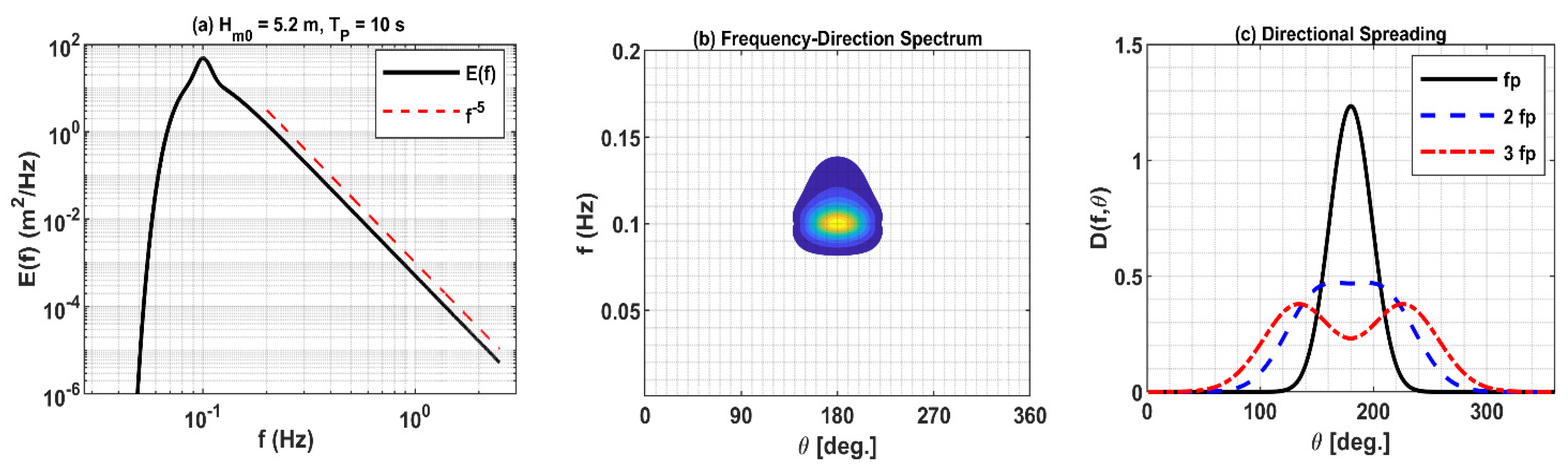
3.1. Surface Wave Simulations

Linear simulations are performed to produce water surface regions with a spatial resolution of 0.01 m and area approximately equal to the footprints of the Radar ($5 \mathrm{m}\times 5 \mathrm{m}$) and the Laser ($0.15 \mathrm{m}\times 0.15 \mathrm{m}$) using linear numerical (Fourier) modeling (Figure 1). For both the instruments, JONSWAP spectra representing wave fields of significant wave heights ($H_{m0}$) 5.2 m, 1.1 m, and 5.8 m, and corresponding peak frequencies ($f_P$) of 0.1 Hz, 0.22 Hz, and 0.07 Hz, with bimodal directional spreading [41] and 1° directional resolution, are used as input to the simulations. The water depth is 125 m. The swell simulations (third case) are run using the JONSWAP parameterization proposed in [42] with peak enhancement factors ($\gamma$) for swell and wind components of 15.0 and 3.3, respectively. The frequency resolution and range for the simulations are chosen to provide a time series of 4096 points with a time step of 0.2 s (5 Hz sampling frequency). The one-dimensional frequency spectrum (Figure 2a), frequency-direction spectrum (Figure 2b), and directional distribution at $f_P$, 2$f_P$, and 3$f_P$ (Figure 3c) representing the wave field of sea states with 5.2 m significant wave height ($H_{m0}$) and peak wave period of 10 s, are given in Figure 2. The color contours in Figure 2b represent spectral energy density in m² Hz⁻¹ deg⁻¹.

3.2. Radar and Laser Simulations

The simulations of the Radar and Laser returns from the water surface follow the laws of reflection and involve a number of modeling steps defined by the design parameters for Radar antenna, the range to points at the sea surface at an instant of time, the modeled attenuation as a function of range, and modeled surface reflection from each point on the surface. Because of the small footprint (0.15 m diameter), the effect of the antenna beam pattern is not considered for the Laser simulations. Both the Lase and Radar simulations use an ideal diffuse reflector, which is termed a Lambertian reflector, producing the same reflection intensity signals at all reflection angles. In numerical simulations, the Lambertian reflection is used as a model for diffuse reflection [43]. However, according to [13], all reflector types (Lambertian, Diffuse, and Specular) produce similar spectral energy levels for frequencies up to 0.8 Hz. The maximum reflection is expected at zero degrees. The complete signal processing method is described in [13]. The basic steps involved in the Radar and Laser simulations are summarized as follows:

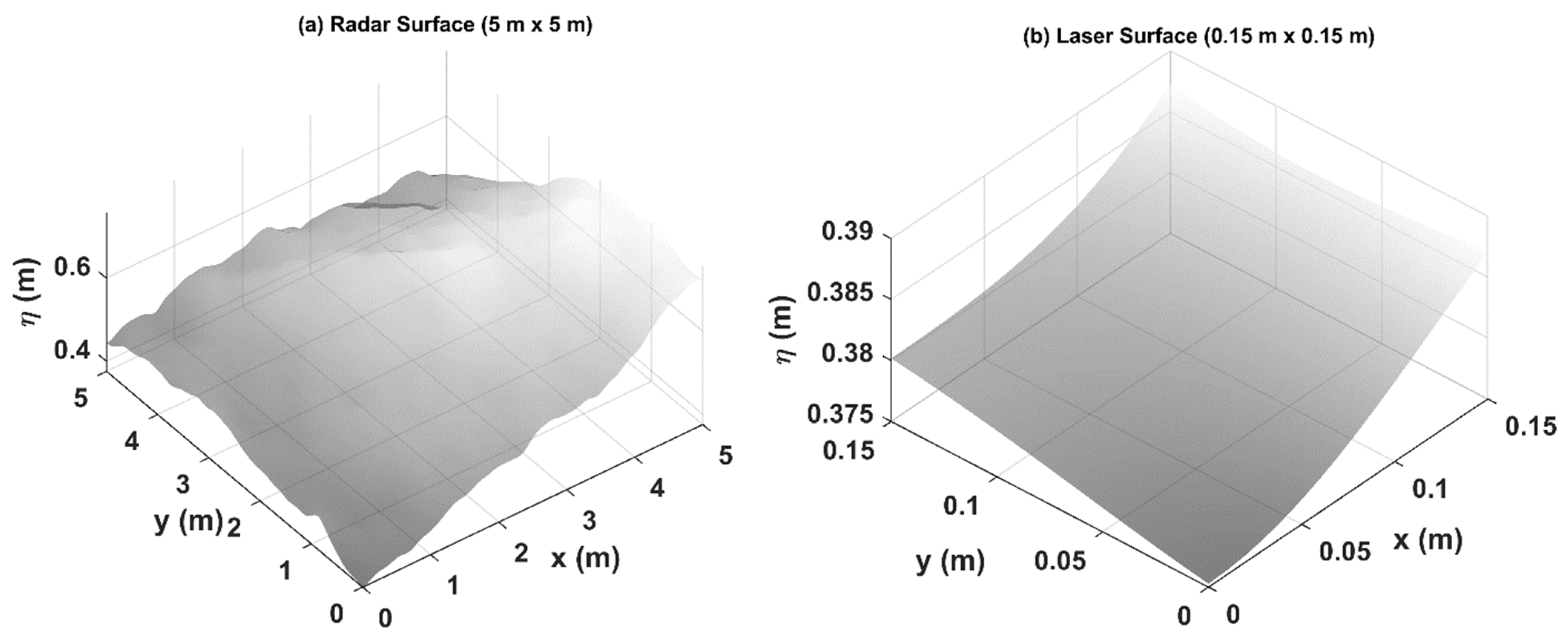
• At each time step, simulated water surface regions (footprints) of the Radar ($5 \mathrm{m}\times 5 \mathrm{m}$) and the Laser ($0.15 \mathrm{m}\times 0.15 \mathrm{m}$) (Figure 1) with a spatial resolution of 0.01 m having a total of 251,001 and 256 grid points, respectively, are converted into a coordinate matrix.
• The location of the Radar and the Laser is fixed in space at the coordinate origin (0,0,0), located horizontally at the center of the water surface (footprint), and 30 m above mean water level for these simulations.
• The distance, $r,$ of each grid point from the position of the instrument is calculated from the geometry.
• At each time step, the signal strength $\left(E\right)$ in terms of gain (intensity), which is a function of range $\left(r\right)$ and beam divergence angle $\left(\theta \right),$ is given as: $E_i\left(x_i,y_i,z_i\right)=E\left({\theta }_i\right)A\left(2r_i\right)R\left({\theta }_i\right)$, where $E\left({\theta }_i\right)$ is the signal strength at the angle ${\theta }_i$ subtended by the point $x_i,y_i,z_i$ to downward vertical at the antenna location (0,0,0), where $z_i=\eta \left(x_i,y_i\right)$. $A\left(2r_i\right)$ is the gain attenuation associated with the path loss over the range ($r_i)$. $R\left({\theta }_i\right)$ is the diffuse reflection coefficient.
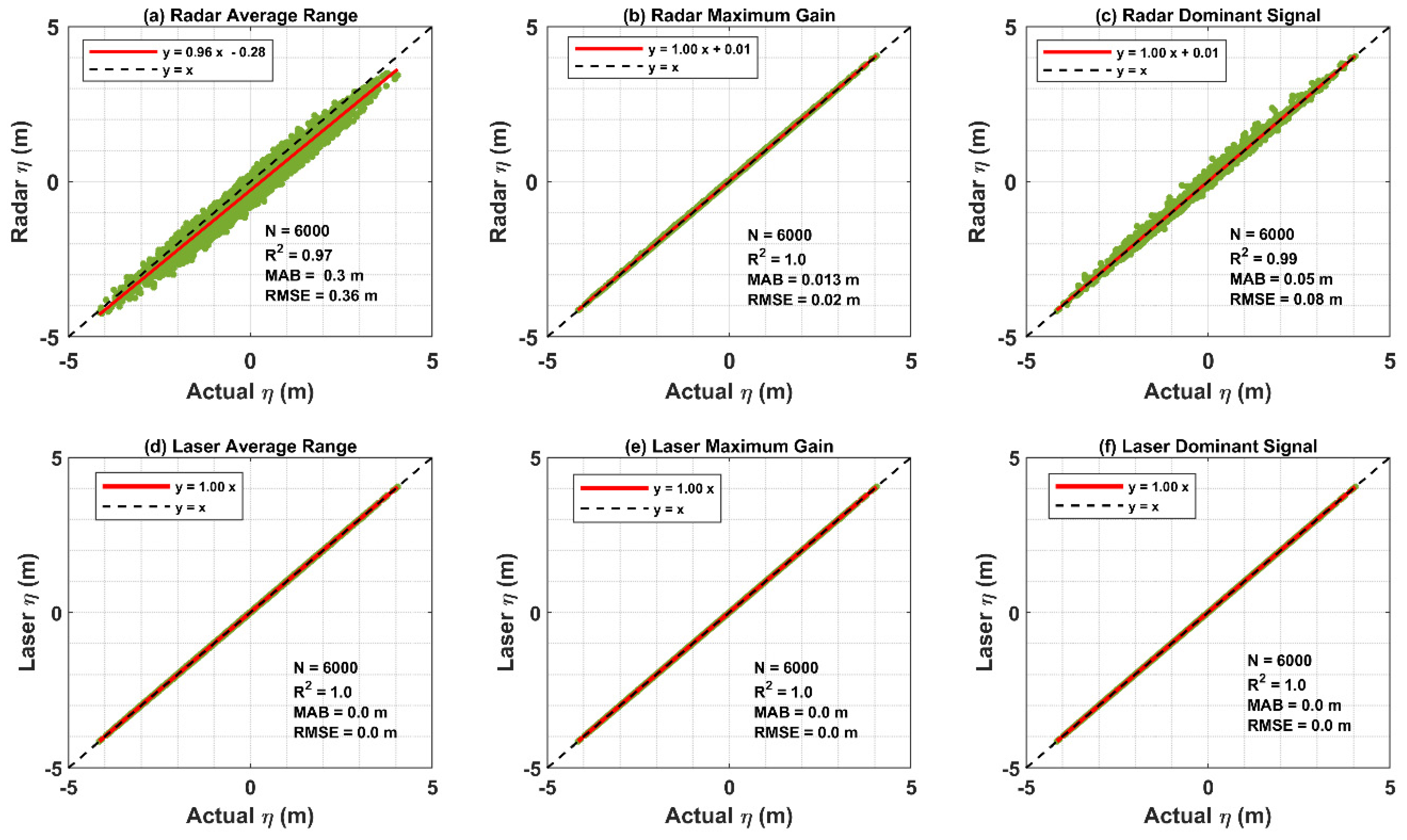
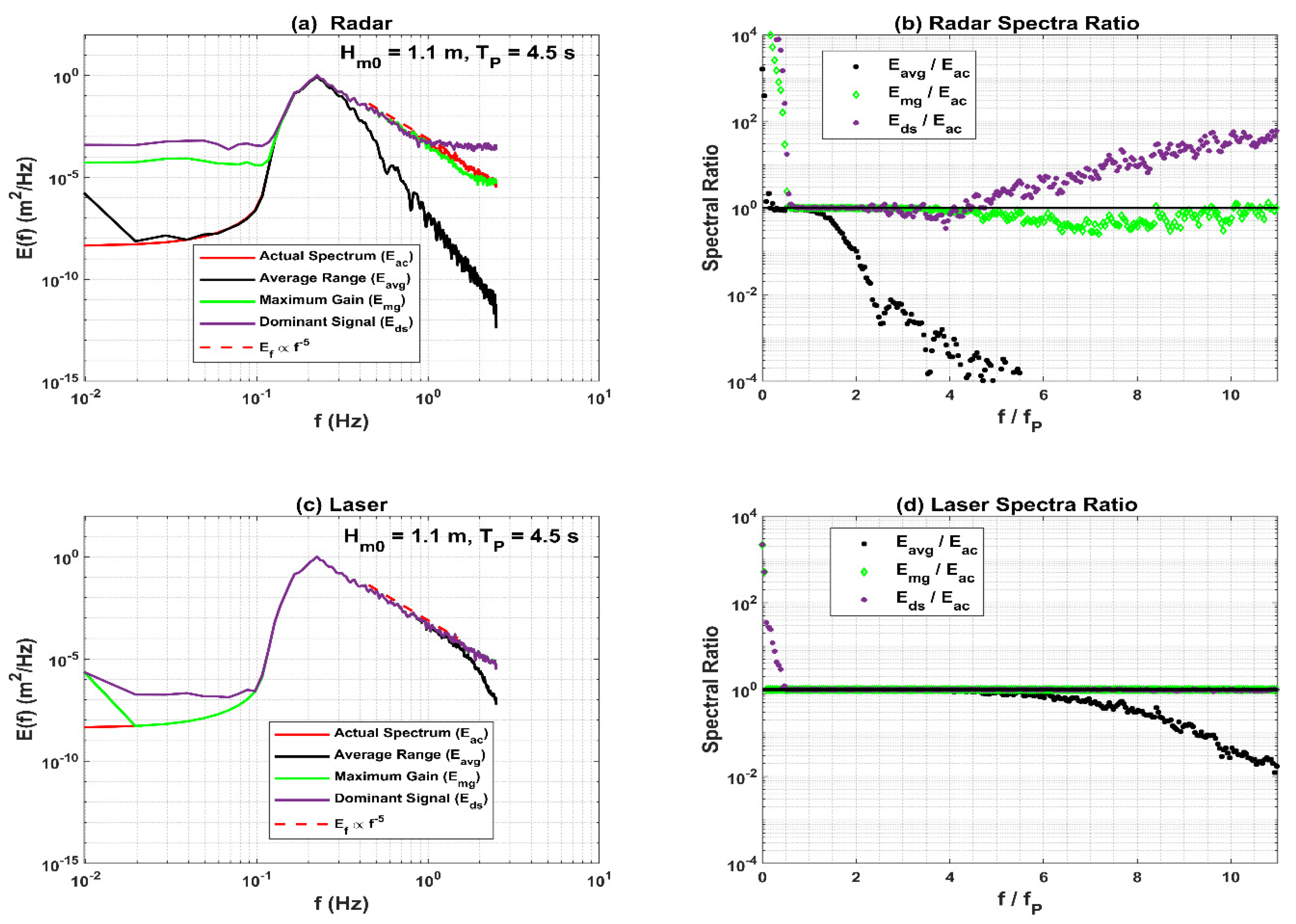
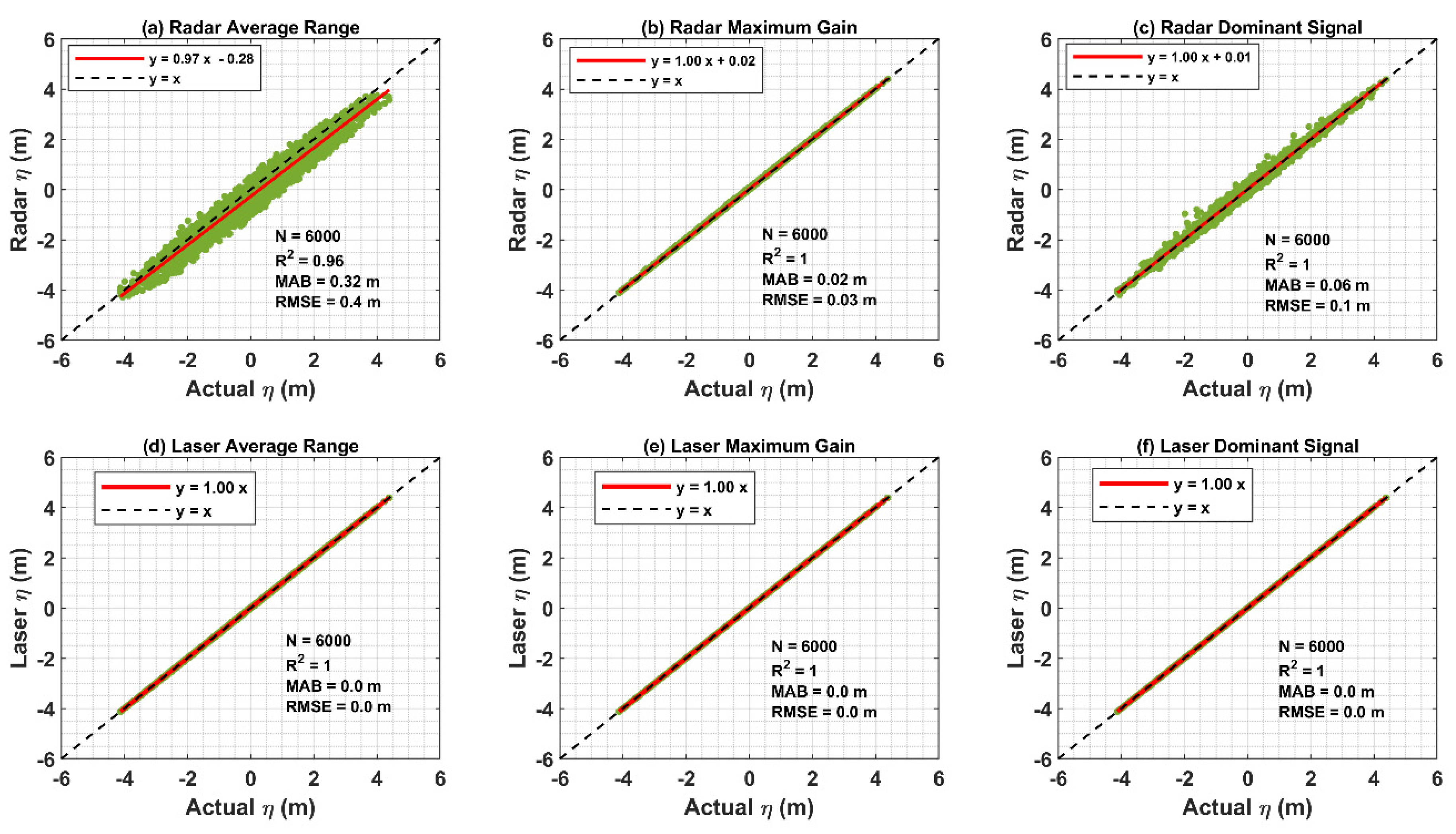
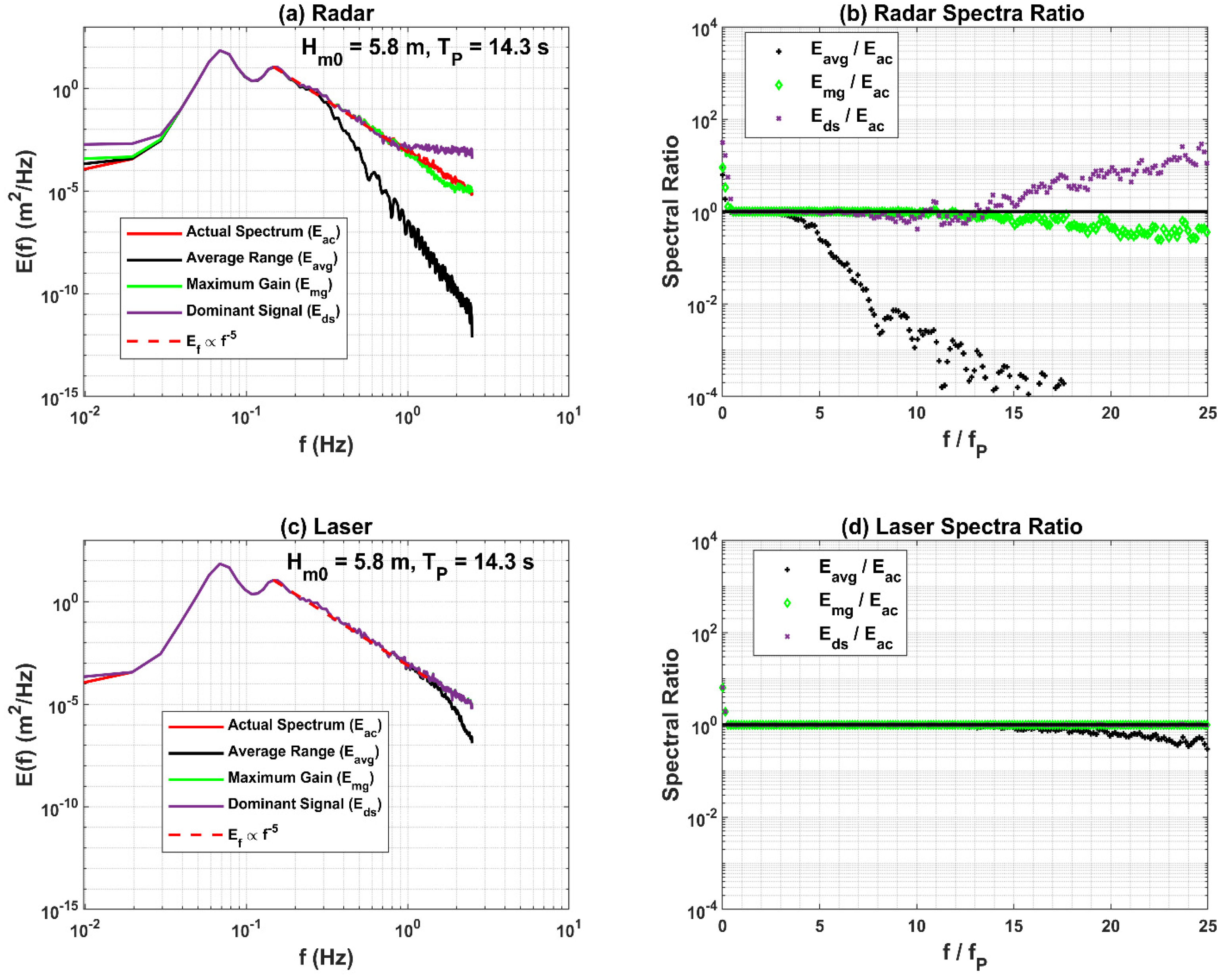
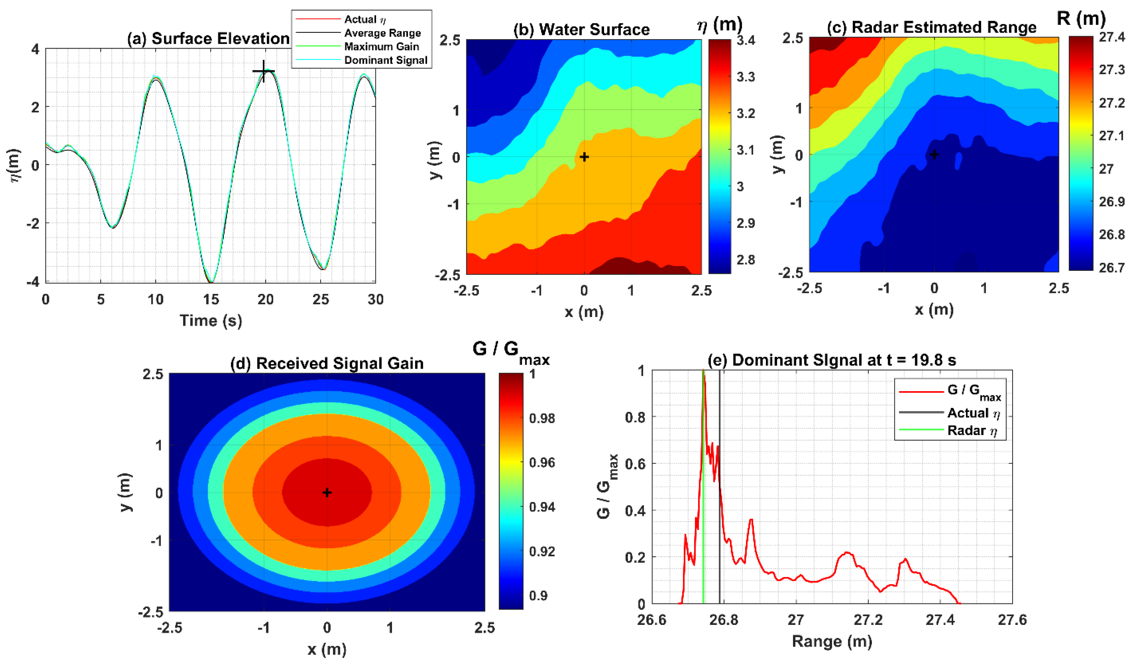
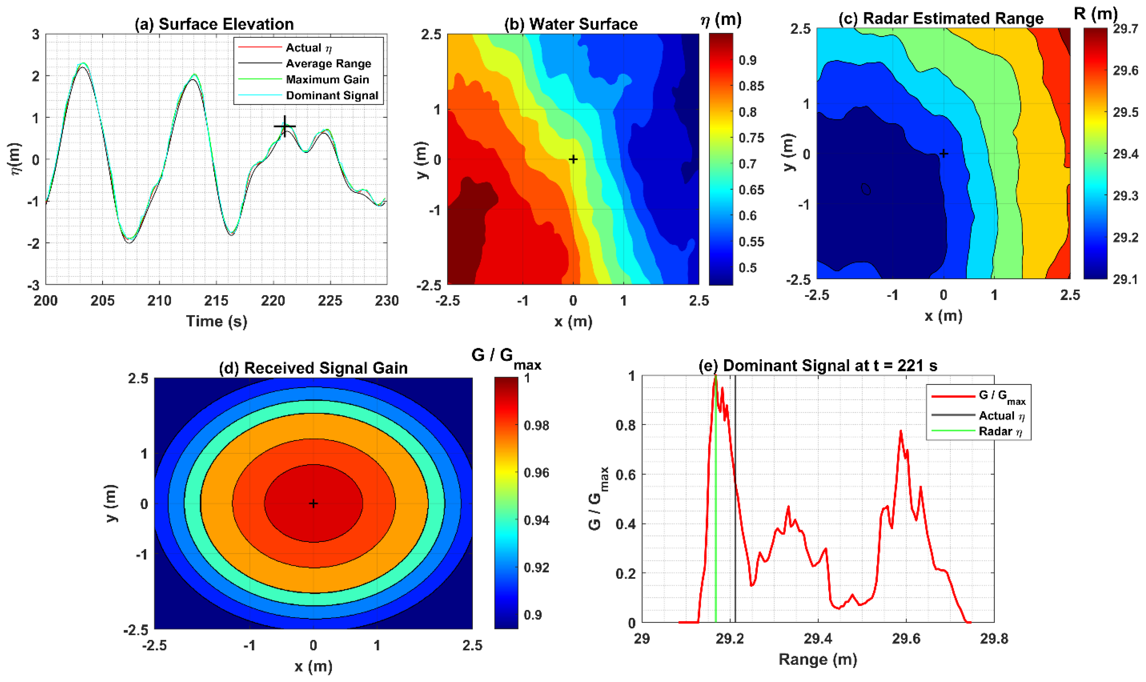
• The reflected signals at each time step are ordered in terms of range, and a cumulative sum of the gains is calculated. The cumulative sum is smoothed, and the density function is derived. The estimated surface elevation is associated with the maximum of the density function. We call this signal the dominant signal (dominant range).
• Additionally, we record the averaged signal, which is the mean of the ranges estimated at each time step.
• As discussed, we have gain values for each range at each time step. We record the signal associated with the maximum gain, which is called the maximum gain signal (not maximum of the density function).
• We compare these simulated signal elevations with the actual surface elevations at the Radar and Laser locations of the water surface (0,0). The actual surface elevations are the time series of surface elevations produced from linear simulations at the positions of the instruments (0,0).

4. Results and Discussion

4.1. Actual Surface Elevation vs. Radar and Laser Simulation

This section compares actual surface elevations with the Radar and Laser simulated surface elevations for three different wind sea and swell conditions. The Radar and Laser simulations include surface elevations estimated from averaged signals (Average Range), maximum gain, and dominant signals processed over their footprints. All three signals are compared against actual surface elevations in time and frequency domains. The power spectral density is computed using the Welch method [44], with a Blackman–Harris window and 50% overlap. First, we examine the performance of the Radar and Laser for a higher sea state representing significant wave height $\left(H_{m0}\right)$ of 5.2 m and peak frequency ($f_P$) 0.1 Hz, and then for a relatively low sea state with $H_{m0}$ and $f_P$ equal to 1.1 m and 0.22 Hz, respectively. Next, we investigate their performance for a swell component with a significant wave height ($H_{m0}$) of 5.8 m and peak frequency ($f_P$) of 0.07 Hz. These simulations indicate how the footprints of the Radar and Laser might affect their performance for varying wind–sea and swell conditions.

4.1.1. High Sea State: $H_{m0}$ = 5.2 m, $f_P$ = 0.10 Hz, $ka=0.104$

Figure 3a–c compare actual surface elevations derived from the simulated water surfaces produced at the horizontal location (0,0) of the vertical to the Radar with the average range and, ranges associated with the maximum gain, and dominant signals over the Radar footprint (water surface of size $5 \mathrm{m}\times 5 \mathrm{m}$) representing a sea state of significant wave height ($H_{m0}$) of 5.2 m and peak frequency of 0.1 Hz, respectively. A similar comparison for the Laser (footprint: $0.15 \mathrm{m}\times 0.15 \mathrm{m}$) is given in Figure 3d–f (for more details, see Section 3.2). The comparisons are made using scatter plots with summary statistics in terms of a total number of data points (N), coefficient of determination (R²), mean absolute bias (MAB) and root mean square error (RMSE).

Figure 3 shows that actual surface elevations ($\eta$) are in excellent agreement with the surface elevations associated with the maximum gain over its footprint (RMSE = 0.02 m) (Figure 3b). The dominant signal (Figure 3c) also agrees well with actual surface elevations compared to the averaged ranges (Figure 3a). The scatter is clearly higher for the averaged signal compared to the other three signals, and as indicated by the RMSE values (Average range RMSE = 0.36 m, Maximum gain RMSE = 0.02 m, Dominant Signal RMSE = 0.08 m). The study in [13] reported that the Radar measures the ranges associated with the dominant signal (maximum of the density function derived), but these simulations suggest that its measurement accuracy would be increased if the signal associated with the direct maximum gain is used (not with the maximum of the density function). However, given such a large footprint and the associated backscatter, the signal maximum is practically not possible to measure with any degree of accuracy and is given only for comparison. On the other hand, because of the significantly smaller footprint (diameter = 0.15 m), all three signals of the Laser provide very accurate estimates of the actual surface elevations (Figure 3d–f). The effect of the reduced beam width is clear in Figure 3a,d, showing the surface elevation from the Laser averaged ranges are in much better agreement with the actual surface elevations ($\eta$) than those from the Radar.

To examine these signals in the frequency domain, Figure 4 compares one-dimensional frequency spectra estimated using surface elevations from averaged ranges, maximum gain, and dominant signals derived from the Radar (Figure 4a) and Laser (Figure 4c) simulations. In Figure 4b,d, we present ratios of spectral energy estimated from averaged ranges (E_avg), maximum gain (E_mg), and dominant signal (E_ds) to the spectral energy estimated using actual surface elevations referred to as the actual spectrum (E_ac), denoted by a black plus (+), green diamond, and purple cross (x) markers, respectively. The ratios are compared as a function of $\frac{f}{f_P}$, where $f_P$ is the peak frequency in Hz.

Figure 4 shows that the Radar dominant signal spectral levels agree well with those of the actual spectrum for frequencies up to 0.5 Hz $\left(\frac{f}{f_P}\approx 5\right)$, but between 0.5 Hz to 1 Hz $\left(\frac{f}{f_P}\approx 10\right)$, it slightly underestimates the spectral levels (purple marker in Figure 4b). Due to the significantly large footprint (diameter = 5.25 m), at higher frequencies, this underestimation is conjectured to be caused by the higher frequencies affecting the gain distribution of the Radar signal, resulting in the estimated range being lower than the actual range. Such behavior was observed for the Radar signals at specific time steps when crests were relatively lower, and troughs were deeper. The overestimation above 1 Hz might be caused by higher frequencies affecting the distribution of signal gain over the Radar footprint. Interestingly, the results from the dominant signal of the Radar agree well with field measurements compared to the Waverider examined in [16,23,24] and agree well with what was reported by [13]. These simulations suggest that the Radar performance, however, can be improved if the Radar provides the ranges associated with the maximum gain signal (not with the maximum of the density function) as it reproduces the spectral levels of the actual spectrum with superior accuracy for frequencies up to 1.2 Hz $\left(\frac{f}{f_P}\approx 12\right)$ (green markers in Figure 4b). However, as discussed above, this signal cannot practically be measured. The spectral levels from the averaged ranges (black marker in Figure 4b) are significantly lower than the actual spectral levels for frequencies above 0.28 Hz $\left(\frac{f}{f_P}\approx 2.8\right)$, which suggests that if the Radar performed averaging of the signals over its footprint, it would provide inaccurate measurement above 0.28 Hz, which does not agree with the results from field measurements [16,23,24]. These studies have reported Radar spectral levels for frequencies above 0.25 Hz being lower than the Waverider by only approximately 10%, compared with an underestimation of more than 50% in case of the simulations. This difference further increases at higher frequencies (more than 100%). A common misconception is that the measurements are representative of an average over the footprint, but it is clear that the results here show how this would result in large inaccuracies.

Figure 4c,d suggest that spectral levels from all three signals processed over the Laser footprint (0.15 m $\times$ 0.15 m) are in very good agreement with those from the actual surface elevations (actual spectrum) over the entire frequency range (up to 2.5 Hz). However, the spectral levels from the averaged signal underestimate above 1.5 Hz.

These simulations suggest that for sea states with significant wave heights ($H_{m0}$) and peak wave periods around 5 m and 10 s, respectively, the footprint affects the wave measurements made at frequencies above approximately 0.5 Hz. This suggests that, at higher frequencies, the Laser measurements might be expected to be more reliable compared to the Radar. Similar results were observed for linear simulations derived for a sea state with $H_{m0}$ and peak wave period of 6.3 m and 10 s, respectively, using the Donelan spectrum [45], which has a high frequency $f^{-4}$ tail, as input. It was found that the underestimation of spectral energy by the Radar for frequencies between 0.5 and 1 Hz for the Donelan spectrum is slightly higher than the JONSWAP spectrum, as given in Figure 4b.

4.1.2. Low Sea State: $H_{m0}$ = 1.1 m, $f_P$ = 0.22 Hz, $ka=0.109$

A similar comparison of the Radar and Laser performance at a relatively low sea state is given in Figure 5 and Figure 6. Figure 5 suggests that at lower sea states, the performance of the Radar slightly decreases as the dominant signal (Figure 5c) agreement with the actual surface elevations is relatively weaker compared to that at higher sea states (see Figure 3c). The performance of the averaged signal also decreases (Figure 5a). However, the Radar maximum gain signal performance is almost unchanged (Figure 5b). Again, this suggests that if the Radar could measure the range associated with the maximum intensity (gain) over its footprint, it could reproduce the actual surface elevations with the highest accuracy in both low and high sea states. The surface elevation estimates for this sea state, from all three Laser signals (Figure 5d–f) compare closely with the actual surface elevations, which may be a consequence of the small sea surface footprint (0.15 m) (Figure 5d–f).

Examining these trends in the frequency domain (Figure 6), the ratios of the spectral levels from the simulated signals to the actual spectral levels show that the spectral levels from the Radar dominant signal agree well with the actual spectral levels for frequencies up to 3.5 times the peak frequency ($f=3.5 f_P=3.5\times 0.22=0.77 \mathrm{Hz}$) (Figure 6b). Above $\frac{f}{f_P}\approx 4$, the dominant signal spectral levels are significantly higher than the actual spectral levels. As shown in Figure 5, the performance of the maximum gain signal is relatively better than the dominant signal. However, at frequencies above five times the peak frequency, its spectral levels are slightly lower than the actual spectral levels. The spectral levels from the averaged ranges agree well with actual spectral levels for frequencies up to approximately 1.5 times the peak frequency (1.5 $\times$ 0.22 = 0.33 Hz). Above 0.33 Hz, the averaged signal underestimates the spectral levels.

4.1.3. Swell: $H_{m0}$ = 5.8 m, $f_P$ = 0.07 Hz, $ka=0.057$

Similarly, we examine the Radar and Laser performance for a swell dominating sea state with a significant wave height ($H_{m0}$) and peak frequency ($f_P$) of 5.8 m and 0.07 Hz, respectively (Figure 7 and Figure 8). Figure 7 and Figure 8 indicate that all three Radar signals (averaged, maximum gain, and dominant) compare relatively well with the actual surface elevations (Figure 7a–c) and their spectral levels (Figure 8). Both in time and frequency domains compared well to the wind sea state conditions, particularly the high sea state (Figure 3 and Figure 5). The dominant and maximum gain spectral levels agree well with actual spectral levels for almost the frequency range, $\left(\frac{f}{f_P}=18\right)$. However, the averaged (Figure 7a) and dominant signal RMSE values shown in scatter plots (Figure 7a,c) are slightly larger than the results for high and low wind-sea states (Figure 3 and Figure 5), but their spectral performance is slightly better (the differences are lower than seen in the wind sea states) (Figure 7 and Figure 8). The values of RMSE and mean absolute bias (MAB) increase with the increase in the significant wave height (Swell > High Sea State > Low Sea State), particularly for the Radar averaged and dominant signals. As above, all three Laser signals compare well with the actual surface elevations, both in time and frequency domains (Figure 7d–f and Figure 8). Overall, the results for both instruments are almost the same.

In summary, these simulations suggest that at higher sea states (Figure 3 and Figure 4), the Radar’s dominant signal performs well for frequencies up to 0.5 Hz ($f=5f_P=0.5$ Hz); however, above 0.5 Hz, it underestimates the spectral levels, which is believed to be caused by its relatively large footprint (5.25 m diameter, when sensor is 30 m above mean water level), affecting signal gain distribution at the sea surface, particularly at higher frequencies. At lower sea states (Figure 5 and Figure 6), its performance slightly decreases (shown by increased scatter in Figure 5); however, its spectral levels still agree well with those from actual surface elevations for frequencies up to 3.5 times the peak frequency ($f=3.5f_P=0.77 \mathrm{Hz}$) (Figure 6). Notably, the Radar performance is superior for the swell dominating higher sea state (Figure 7 and Figure 8): performing well for frequencies up to 15 times the peak frequency ($f=15f_P=1.05 \mathrm{Hz}$). All three Laser signals compare well with actual surface elevations due to the tiny footprint (0.15 m), irrespective of the sea states, but the simulations suggest that the footprint size might affect wave measurements made at frequencies above 0.5 Hz. We believe the spectral energy overestimation (2–3%) by Laser, and as found also in [16], is associated with the poor quality of the Laser data used for the analysis. The Laser data must go through an exhaustive quality control procedure before a detailed analysis can be performed [23]. In addition, the simulations confirm that the Radar does not perform averaging over its footprint, also substantiated by [13], contrary to what has sometimes been speculated (that the Radar provides averaged ranges over its footprint), e.g., in [15].

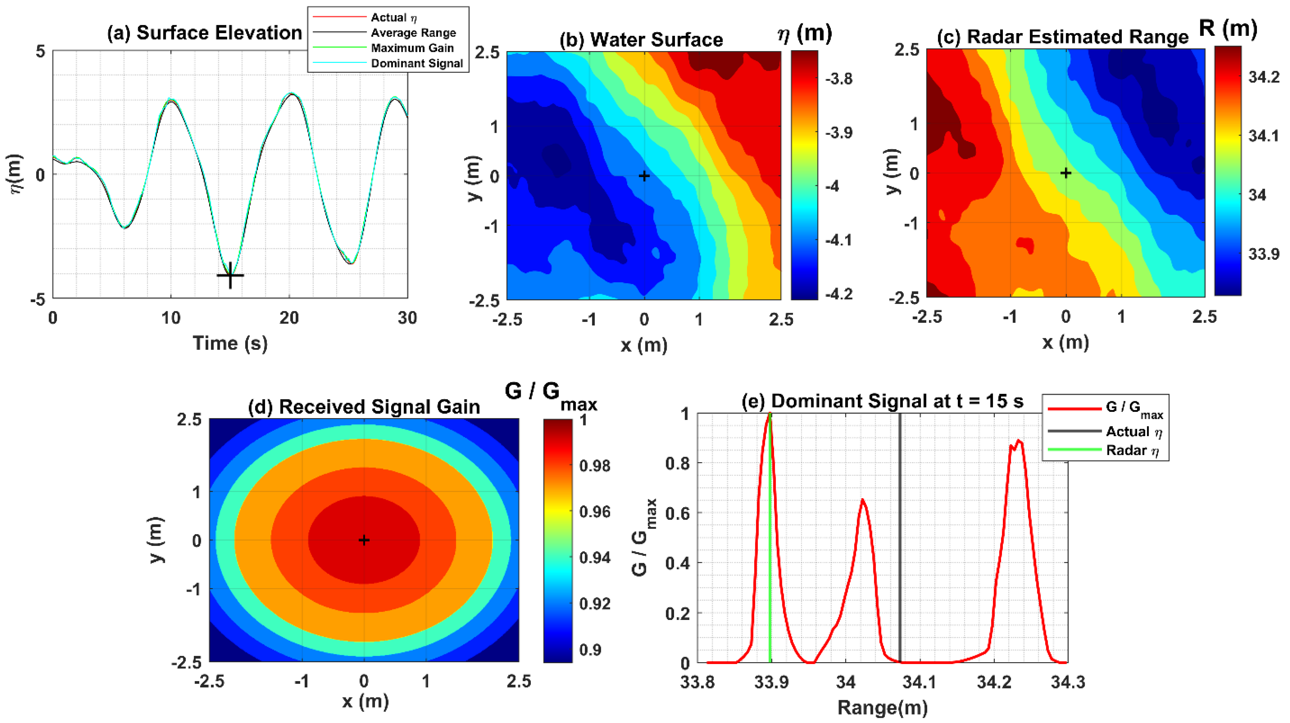
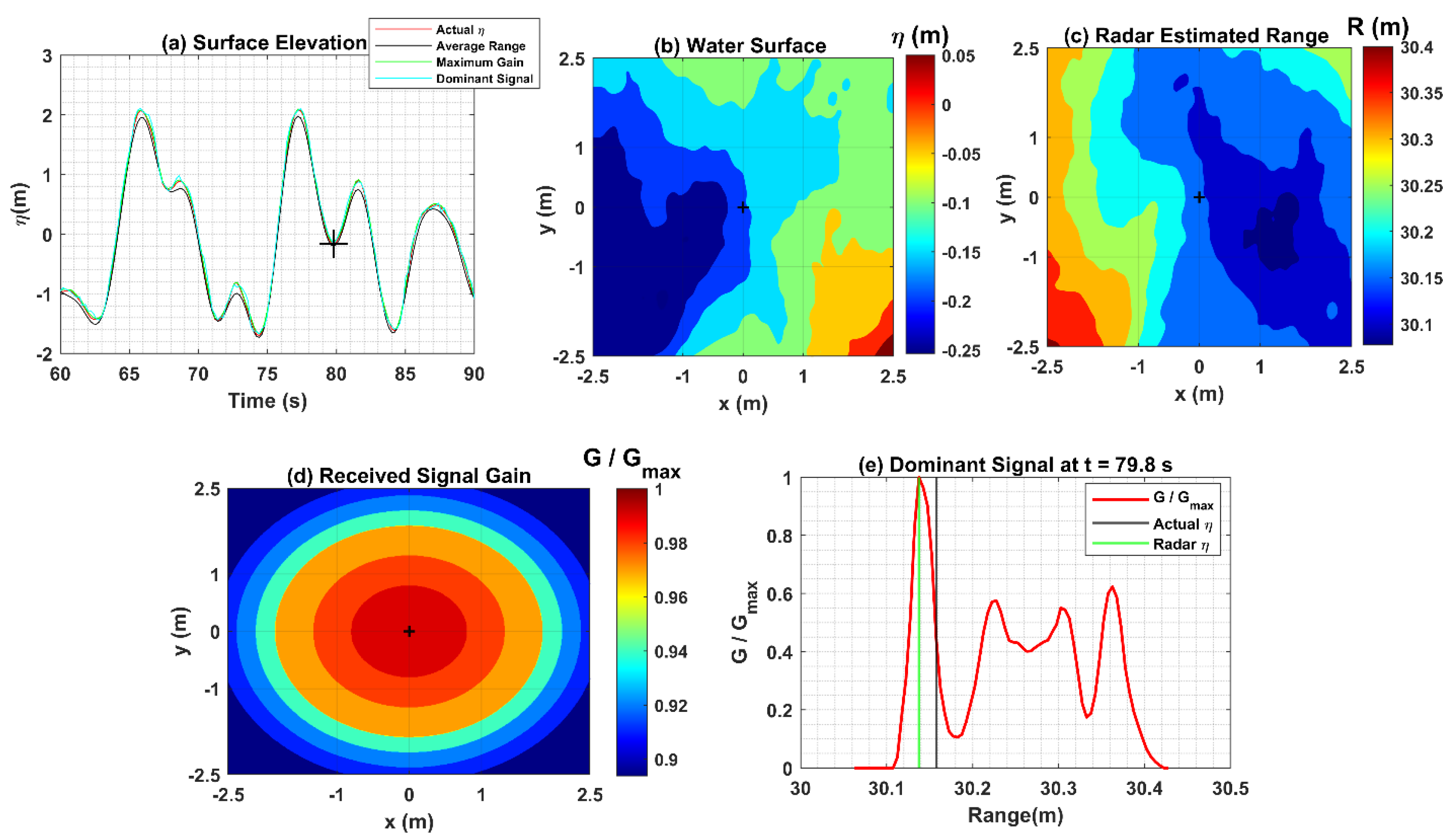
4.2. Radar Dominant Signal at Specific Time Steps

Ref. [13] modelled the Radar using the dominant signal to measure the vertical distance to the sea surface. In the sections above, we have investigated three different models for the signal processed over water surfaces of sizes 5 m $\times$ 5 m at each time step, including the dominant, but the analysis above does not provide details on how the dominant signal gain distribution is affected for specific surface elevations around crests and troughs as a function of range. Therefore, in this section, we examine the dominant signal gain distribution and associated range, comparing it with actual surface elevation ($\eta$), for two relatively different crests: 3.2 m and 0.78 m, and troughs: −4.1 m and −0.2 m, which occurred at 19.8, 221, 15, and 79.8 s, respectively, from the start of the record of the high sea state condition (Figure 3 and Figure 4). In all four cases, each figure has time series plots of the actual surface elevation ($\eta$), average range, maximum gain, and dominant signal with black plus (+) marker, indicating the crest or trough vertically below the sensor location. Color contour plots show the water surface and Radar range over its footprint (5 m $\times$ 5 m) with black plus (+) markers at the center, indicating the crest or trough at that time step. A color contour plot shows the normalized received signal gain (G/G_max) over the Radar footprint. The normalized dominant signal gain is shown as a function of range with green and black lines indicating the ranges associated with the maximum of the gain density function (solid red line) (Radar $\eta$) and actual surface elevation (actual $\eta$) denoted by the black plus (+) markers in time series and all color contour plots. The (0,0) is the location of the Radar in space.

The Radar signal reflections using the antenna beam pattern (see [13]) are processed over these water surfaces; the ranges are estimated using geometry and received signal gain (G) from the equation, $E\left(x,y,z\right)=E\left(\theta \right)A\left(2r\right)R\left(\theta \right)$ (described in Section 3.2), and are normalized by dividing by the maximum gain (G_max). The estimated ranges and normalized received signal gain are shown in the color contour plots separately at 19.8 and 221 s. Figure 9d and Figure 10d indicate that the maximum gain is at the center, the location of the Radar (0,0) or at zero degrees divergence angle, which, as per the antenna beam pattern, is accurate. The cumulative sum of the received signal gain is estimated, smoothed, and a density function is derived. The normalized signal gain density function (G/G_max) as a function of the range is given in Figure 9e and Figure 10e at these crest elevations. The range associated with the maximum of the density function derived is measured by the Radar (solid green line) and is called the dominant signal. The solid black line is the range (30 − 3.21 = 26.79 m) associated with the actual surface elevation ($\eta =3.21$ m) expected to be measured by the Radar.

4.2.1. Crest Elevations

Figure 9 and Figure 10 represent the Radar full signal processing to measure a crest elevation of 3.2 m and 0.78 m occurring at 19.8 and 221 s, respectively, shown by black plus (+) markers in the time series plots (Figure 9a and Figure 10a).

As per the antenna Received Signal Gain beam pattern, the Radar has its maximum signal intensity (gain) underneath the sensor at zero degrees beam divergence angle (Figure 9d and Figure 10d center). The Radar antenna signal intensity decreases at angles away from the antenna center (see Figure 4 in ref [13]). Figure 9e and Figure 10e show that the maximum of the dominant signal gain (G/G_max = 1) occurs at a slightly shorter range than the actual position of the Radar (0,0) (solid black lines), resulting in a slightly larger value of surface elevation than the actual. It is possible that this is caused by the change in position of the highly intense signal over the large Radar footprint, probably associated with the crest that occurs a second or so later. Given the inherent inaccuracies with the simulations, minor deviations in the signal gain distribution are expected. For a 3.2 m high crest, the dominant signal gain is appropriately distributed as per the Radar antenna beam pattern, decreasing with the increase in the range away from the Radar position (0,0) (Figure 9e). However, for a relatively small 0.78 m high crest, the signal gain decreases with an increase in the range up to 29.5 m (Figure 10), but after this, it again significantly increases and then decreases towards the range end. It appears the Radar antenna beam pattern has two separate maxima over its footprint, suggesting the Radar signal gain might not be appropriately distributed for such small crests over such a large footprint. For such small crests, path loss over range increases, which decreases the intensity of the reflected signal. Therefore, the high-intensity signal might not be underneath the Radar at zero degrees angle and would result in the selection of a point away from the actual position of the Radar (0,0). For smaller crests, the change in the angle of reflection might also affect the position of the high-intensity signal.

4.2.2. Trough Depths

The dominant signal is similarly examined for two relatively different troughs with depths of −4.1 m and −0.2 m, respectively. The time steps at which these troughs occurred, denoted by black plus (+) markers, are given in the time series plots (Figure 11a and Figure 12a). At these time steps, the water surface regions, estimated ranges, and normalized received signal gains over the Radar footprint are shown using color contours in Figure 11b–d (−4.1 m) and Figure 12b–d (−0.2 m). For these troughs, the processed normalized dominant signal gains as a function of the range are given in Figure 11e and Figure 12e.

As seen in Figure 11d and Figure 12d, the maximum signal intensity (gain) is at the location of the Radar (0,0) (black plus (+) at the center) corresponding to the surface elevations at the centers of the water surface regions shown in Figure 11b and Figure 12b. The ranges corresponding to these surface elevations are shown at the centers of Figure 11c and Figure 12c and solid black lines in Figure 11e and Figure 12e, which are expected to be provided by the dominant signal. However, these figures suggest that the ranges corresponding to the maximum of the normalized signal gain density function (solid green) are slightly different from the actual ranges (solid black). The difference is higher for the relatively deeper trough (Figure 11e). In a similar manner to that observed for the 0.78 m crest elevation, the signal gain distribution for these troughs does not follow the Radar received signal beam pattern (antenna beam pattern). The signal gain fluctuates with an increase in the range, indicated by several peaks (gain maximum) over its footprint due to the attenuation associated with loss over range and the change in reflection angle with wave slope. This problem is relatively more pronounced for the deeper trough (depth = −4.1 m).

In summary, the dominant signal follows the Radar beam antenna pattern accurately for the 3.2 m high crest, which corresponds to the lowest range (Range = 30 − 3.2 = 26.8 m) (Figure 9e). However, for the deepest trough (depth −4.1 m) corresponding to the highest range (Range = 30 − (−4.1) = 34.1 m) (Figure 11e), it does not follow the Radar antenna beam pattern accurately. The dominant signal gain distribution is approximately the same for the 0.78 m high crest (Range = 30 − 0.78 = 29.22 m) (Figure 10e) and −0.2 m deep trough (Range = 30 − (−0.2) = 30.2 m) (Figure 12e), both partially following the Radar antenna beam pattern. This analysis suggests that the dominant Received Signal Gain distribution deviates from the Radar antenna beam pattern at higher ranges. This might be caused by the increase in path loss (gain loss) over range, decreasing the overall signal intensity at higher ranges [13], suggesting the Radar dominant signal will provide relatively better measurements of higher crests (low range) compared to lower crests and deeper troughs (high range). The path loss over range might also be responsible for why the Radar underestimates spectral levels for frequencies above 0.5 Hz (see Section 4.1). In all four cases, the Radar ranges are slightly lower than the actual ranges (underestimating), indicated by the solid green and black lines (Figure 9e, Figure 10e, Figure 11e and Figure 12e), respectively, which is a consequence of the antenna beam width, and due to the highly attenuated signal with azimuth. The effective footprint is small in comparison to that estimated from the beam width.

5. Conclusions

This paper presents the results of an investigation of wave measurement principles of a Rosemount WaveRadar (Radar) and an Optech^TM Laser (Laser) using linear simulations. Their simulations are based on the approach described in [13], which includes modeling the electromagnetic signal reflections from the water surface to estimate the range (vertical distance) for sensors located at a 30 m height from the sea surface. The simulations are performed for two relatively steep wind seas (1. $H_{m0}$= 5.2 m, $T_P$ = 10 s, $ka$ = 0.104, 2. $H_{m0 }$= 1.1 m, $T_P$ = 4.5 s, $ka$ = 0.109) and a swell (3. $H_{m0}$= 5.8 m, $T_P$ = 14.3 s, $ka$ = 0.057) condition.

The Laser and Radar simulations confirm the dominant signal, which is believed to be the signal that the radar measurements record, performs well for frequencies up to 0.5 Hz. However, above 0.5 Hz, Radar underestimates the actual spectral levels (Figure 4b, Figure 6b and Figure 8b). Its performance is slightly better for the swell condition (up to 0.77 Hz) (Figure 8b). Due to the relatively smaller footprint (0.15 m), all three Laser signals perform well for almost the entire frequency range for all three cases (Figure 4d, Figure 6d and Figure 8d). This is consistent with the decreased performance of the Radar dominant signal at higher frequencies, resulting from the significantly larger footprint (5.25 m) at the sea surface. This affects the signal gain distribution by randomly shifting the maximum of density function. Another consequence of the larger footprint is that at higher ranges (smaller crests or troughs), the dominant signal does not follow the Radar antenna beam pattern as accurately as the lower ranges (higher crests). At higher ranges (smaller waves), the signal path loss increases [13], and there is increased reflected signal returns at a larger distance from the vertical to the sensor.

References

1. Measuring Ocean Waves: Proceedings of a Symposium and Workshop on Wave Measurement Technology; The National Academies Press: Washington, DC, USA, 1982.
2. Allender, J.; Audunson, T.; Barstow, S.F.; Bjerken, S.; Krogstad, H.E.; Steinbakke, P.; Vartdal, L.; Borgman, L.E.; Graham, C. The WADIC Project: A Comprehensive Field Evaluation of Directional Wave Instrumentation. Ocean. Eng. 1989, 16, 505–536. [Google Scholar] [CrossRef]
3. Dysthe, K.; Krogstad, H.E.; Müller, P. Oceanic Rogue Waves. Annu. Rev. Fluid Mech. 2008, 40, 287–310. [Google Scholar] [CrossRef]
4. Young, I.R. Directional Spectra of Hurricane Wind Waves. J. Geophys. Res. Oceans 2006, 111. [Google Scholar] [CrossRef]
5. Young, I.R. On the Measurement of Directional Wave Spectra. Appl. Ocean Res. 1994, 16, 283–294. [Google Scholar] [CrossRef]
6. Banner, M.L.; Young, I.R. Modeling Spectral Dissipation in the Evolution of Wind Waves. Part I: Assessment of Existing Model Performance. J. Phys. Oceanogr. 1994, 24, 1550–1571. [Google Scholar] [CrossRef]
7. Young, I.R.; van Vledder, G.P. A Review of the Central Role of Nonlinear Interactions in Wind—Wave Evolution. Philos. Trans. R. Soc. London. Ser. A Phys. Eng. Sci. 1993, 342, 505–524. [Google Scholar]
8. Young, I.R.; Verhagen, L.A.; Banner, M.L. A Note on the Bimodal Directional Spreading of Fetch-limited Wind Waves. J. Geophys. Res. Ocean 1995, 100, 773–778. [Google Scholar] [CrossRef]
9. Young, I.R.; Zieger, S.; Babanin, A.V. Global Trends in Wind Speed and Wave Height. Science 2011, 332, 451–455. [Google Scholar] [CrossRef]
10. Young, I.R.; Vinoth, J.; Zieger, S.; Babanin, A.V. Investigation of Trends in Extreme Value Wave Height and Wind Speed. J. Geophys. Res. Oceans 2012, 117. [Google Scholar] [CrossRef]
11. Janssen, P.A.E.M.; Hansen, B.; Bidlot, J.-R. Verification of the ECMWF Wave Forecasting System against Buoy and Altimeter Data. Weather 1997, 12, 763–784. [Google Scholar] [CrossRef]
12. Bidlot, J.-R.; Holmes, D.J.; Wittmann, P.A.; Lalbeharry, R.; Chen, H.S. Intercomparison of the Performance of Operational Ocean Wave Forecasting Systems with Buoy Data. Weather 2002, 17, 287–310. [Google Scholar] [CrossRef]
13. Ewans, K.; Feld, G.; Jonathan, P. On Wave Radar Measurement. Ocean Dyn. 2014, 64, 1281–1303. [Google Scholar] [CrossRef]
14. Christou, M.; Ewans, K. Examining a Comprehensive Dataset Containing Thousands of Freak Wave Events: Part 1—Description of the Data and Quality Control Procedure. In Proceedings of the International Conference on Offshore Mechanics and Arctic Engineering, Rotterdam, The Netherlands, 19–24 June 2011; Volume 44342, pp. 815–826. [Google Scholar]
15. Barstow, S.F.; Krogstad, H.E. Procedures and Problems Associated with the Calibration of Wave Sensors. J. Eval. Comp. Calibration Oceanogr. Instrum. Proc. Int. Conf. (Ocean Data) 1985, 4, 55–82. [Google Scholar]
16. Magnusson, A.K.; Jensen, R.; Swail, V. Spectral Shapes and Parameters from Three Different Wave Sensors. Ocean Dyn. 2021, 71, 893–909. [Google Scholar] [CrossRef]
17. Hasselmann, D.E.; Dunckel, M.; Ewing, J.A. Directional Wave Spectra Observed during JONSWAP 1973. J. Phys. Oceanogr. 1980, 10, 1264–1280. [Google Scholar] [CrossRef]
18. Pontes, M.T. Assessing the European Wave Energy Resource. ASME. J. Offshore Mech. Arct. Eng. 1998, 120, 226–231. [Google Scholar] [CrossRef]
19. Fedele, F.; Arena, F. Long-Term Statistics and Extreme Waves of Sea Storms. J. Phys. Oceanogr. 2010, 40, 1106–1117. [Google Scholar] [CrossRef]
20. Lenee-Bluhm, P.; Paasch, R.; Özkan-Haller, H.T. Characterizing the Wave Energy Resource of the US Pacific Northwest. Renew. Energy 2011, 36, 2106–2119. [Google Scholar] [CrossRef]
21. Tucker, M.J.; Pitt, E.G. Waves in Ocean Engineering; The National Academies of Sciences, Engineering, and Medicine: Washington, DC, USA, 2001; ISBN 0080435661. [Google Scholar]
22. Gronlie, O. Wave Radars-a Comparison of Concepts and Techniques. Hydro Int. 2004, 8, 24–27. [Google Scholar]
23. Jangir, P.K.; Ewans, K.; Young, I.R. Comparative Performance of Radar, Laser, and Waverider Buoy measurements of ocean waves—Part 1: Frequency domain Analysis. J. Atmos. Ocean. Technol. 2022; submitted. [Google Scholar]
24. Jangir, P.K.; Ewans, K.; Young, I.R. Comparative Performance of Radar, Laser, and Waverider Buoy measurements of ocean waves—Part 2: Time domain Analysis. J. Atmos. Ocean. Technol. 2022; submitted. [Google Scholar]
25. Noreika, S.; Beardsley, M.; Lodder, L.; Brown, S.; Duncalf, D. Comparison of Contemporaneous Wave Measurements with a Rosemount Waveradar REX and a Datawell Directional Waverider Buoy. In Proceedings of the 12th International Workshop on Wave Hindcasting and Forecasting & 3rd Coastal Hazard Symposium, Kohala Coast, HI, USA, 30 October–4 November 2011. [Google Scholar]
26. Krogstad, H.E.; Wolf, J.; Thompson, S.P.; Wyatt, L.R. Methods for Intercomparison of Wave Measurements. Coast. Eng. 1999, 37, 235–257. [Google Scholar] [CrossRef]
27. Forristall, G.Z.; Barstow, S.F.; Krogstad, H.E.; Prevosto, M.; Taylor, P.H.; Tromans, P.S. Wave Crest Sensor Intercomparison Study: An Overview of WACSIS. J. Offshore Mech. Arct. Eng. 2004, 126, 26–34. [Google Scholar] [CrossRef]
28. Longuet-Higgins, M.S. On the Skewness of Sea-Surface Slopes. J. Phys. Oceanogr. 1982, 12, 1283–1291. [Google Scholar] [CrossRef]
29. James, I.D. A Note on the Theoretical Comparison of Wave Staffs and Wave Rider Buoys in Steep Gravity Waves. Ocean Eng. 1986, 13, 209–214. [Google Scholar] [CrossRef]
30. Srokosz, M.A.; Longuet-Higgins, M.S. On the Skewness of Sea-Surface Elevation. J. Fluid Mech. 1986, 164, 487–497. [Google Scholar] [CrossRef]
31. Longuet-Higgins, M.S. Eulerian and Lagrangian Aspects of Surface Waves. J. Fluid Mech. 1986, 173, 683–707. [Google Scholar] [CrossRef]
32. Forristall, G.Z. Wave Crest Distributions: Observations and Second-Order Theory. J. Phys. Oceanogr. 2000, 30, 1931–1943. [Google Scholar] [CrossRef]
33. Marthinsen, T.; Winterstein, S.R. On the Skewness of Random Surface Waves. In Proceedings of the Second International Offshore and Polar Engineering Conference, San Francisco, CA, USA, 14–19 June 1992. [Google Scholar]
34. Prevosto, M.; Krogstad, H.E.; Robin, A. Probability Distributions for Maximum Wave and Crest Heights. Coast. Eng. 2000, 40, 329–360. [Google Scholar] [CrossRef]
35. McAllister, M.L.; van den Bremer, T.S. Lagrangian Measurement of Steep Directionally Spread Ocean Waves: Second-Order Motion of a Wave-Following Measurement Buoy. J. Phys. Oceanogr. 2019, 49, 3087–3108. [Google Scholar] [CrossRef]
36. Herbers, T.H.C.; Janssen, T.T. Lagrangian Surface Wave Motion and Stokes Drift Fluctuations. J. Phys. Oceanogr. 2016, 46, 1009–1021. [Google Scholar] [CrossRef]
37. Herbers, T.H.C.; Elgar, S.; Guza, R.T. Infragravity-Frequency (0.005–0.05 Hz) Motions on the Shelf. Part I: Forced Waves. J. Phys. Oceanogr. 1994, 24, 917–927. [Google Scholar] [CrossRef]
38. Herbers, T.H.C.; Jessen, P.F.; Janssen, T.T.; Colbert, D.B.; MacMahan, J.H. Observing Ocean Surface Waves with GPS-Tracked Buoys. J. Atmos. Ocean. Technol. 2012, 29, 944–959. [Google Scholar] [CrossRef]
39. Aqua-Ltd. WaveRadar REX Operating and Installation Manual—Issue K1; Rosemount WaveRadar Manual, RS Aqua Ltd.: Scotland, UK, 2014. [Google Scholar]
40. Optech. Sentinal 3100 User Manual DV and CP Models. Available online: https://vdocuments.net/sentinel-3100-user-manual-dv-and-cp-manualsoptech-sentinel-3100-user-manual.html?page=1 (accessed on 17 July 2022).
41. Ewans, K.C. Observations of the Directional Spectrum of Fetch-Limited Waves. J. Phys. Oceanogr. 1998, 28, 495–512. [Google Scholar] [CrossRef]
42. Ewans, K.C.; Bitner-Gregersen, E.M.; Soares, C.G. Estimation of Wind-Sea and Swell Components in a Bimodal Sea State. J. Offshore Mech. Arct. Eng. 2006, 128, 265–270. [Google Scholar] [CrossRef]
43. Sanjeev, J.K. Lambertian Reflectance. In Computer Vision: A Reference Guide; Ikeuchi, K., Ed.; Springer: Boston, MA, USA, 2014; pp. 441–443. [Google Scholar]
44. Welch, P. The Use of Fast Fourier Transform for the Estimation of Power Spectra: A Method Based on Time Averaging over Short, Modified Periodograms. IEEE Trans. Audio Electroacoust. 1967, 15, 70–73. [Google Scholar] [CrossRef] [Green Version]
45. Donelan, M.A.; Hamilton, J.; Hui Mathematical, W.S.A.; Sciences, P. Directional Spectra of Wind-Generated Ocean Waves. Ser. A Math. Phys. Sci. 1985, 315, 509–562. [Google Scholar]
Figure 1. Examples of water surface regions simulated using linear (Fourier) numerical modeling approximately covered by the footprints of (a) the Radar ( 5   m   × 5   m ) and (b) the Laser ( 0.15   m   × 0.15   m ) beams.
Jmse 10 01260 g001
Figure 2. JONSWAP one-dimensional frequency spectrum (a), frequency-direction spectrum (b), and directional spreading (c). The color contours represent spectral energy density in m 2 Hz 1   deg 1 .
Jmse 10 01260 g002
Figure 3. Comparisons of actual surface elevation with average range (a,d), maximum gain (b,e), and dominant signal (c,f) estimated from the Radar and Laser simulations for a sea state with a significant wave height ( H m 0 ) and peak frequency of 5.2 m and 0.1 Hz, respectively.
Jmse 10 01260 g003
Figure 4. Comparison of one-dimensional frequency spectra estimated from actual surface elevations with the spectra derived from the simulated surface elevations of the Radar (a,b) and the Laser (c,d) from averaged ranges, ranges associated with maximum gain and dominant signals for a sea state with a significant wave height ( H m 0 ) and peak frequency of 5.2 m and 0.1 Hz, respectively.
Jmse 10 01260 g004
Figure 5. Comparisons of actual surface elevation with average range (a,d), maximum gain (b,e), and dominant signal (c,f) estimated from the Radar and Laser simulations for a sea state with a significant wave height ( H m 0 ) and peak frequency ( f P ) of 1.1 m and 0.22 Hz, respectively.
Jmse 10 01260 g005
Figure 6. Comparison of one-dimensional frequency spectra estimated from actual surface elevations with the spectra derived from the simulated surface elevations of the Radar (a,b) and the Laser (c,d) from averaged ranges, ranges associated with maximum gain and dominant signals for a sea state with a significant wave height ( H m 0 ) and peak frequency ( f P ) of 1.1 m and 0.22 Hz, respectively.
Jmse 10 01260 g006
Figure 7. Comparisons of actual surface elevation with average range (a,d), maximum gain (b,e), and dominant signal (c,f) estimated from the Radar and Laser simulations for a swell dominating sea state with a significant wave height ( H m 0 ) and peak frequency ( f P ) of 5.8 m and 0.07 Hz, respectively.
Jmse 10 01260 g007
Figure 8. Comparison of one-dimensional frequency spectra estimated from actual surface elevations with the spectra derived from the simulated surface elevations of the Radar (a,b) and the Laser (c,d) from averaged ranges, ranges associated with maximum gain and dominant signals for a swell dominating sea state with a significant wave height ( H m 0 ) and peak frequency ( f P ) of 5.8 m and 0.07 Hz, respectively.
Jmse 10 01260 g008
Figure 9. Radar dominant signal processing for a crest elevation of 3.2 m occurred at 19.8 s: (a) time series plots of actual surface elevations and that from the Radar signals; (b) water surface covered by the Radar footprint (5 m × 5 m); (c) Radar estimated ranges over its footprint; (d) normalized received signal gain over the Radar footprint; (e) normalized dominant signal gain as a function of range.
Jmse 10 01260 g009
Figure 10. Radar dominant signal processing for a crest elevation of 0.78 m which occurred at time step of 221 s: (a) time series plots of actual surface elevations and that from the Radar signals; (b) water surface covered by the Radar footprint (5 m × 5 m); (c) Radar estimated ranges over its footprint; (d) normalized received signal gain over the Radar footprint; (e) normalized dominant signal gain as a function of range.
Jmse 10 01260 g010
Figure 11. Radar dominant signal processing for a trough of depth −4.1 m occurred at a time step of 15 s: (a) time series plots of actual surface elevations and that from the Radar signals; (b) water surface covered by the Radar footprint (5 m × 5 m); (c) Radar estimated ranges over its footprint; (d) normalized received signal gain over the Radar footprint; (e) normalized dominant signal gain as a function of range.
Jmse 10 01260 g011
Figure 12. Radar dominant signal processing for a trough of depth −0.2 m occurred at time step of 79.8 s: (a) time series plots of actual surface elevations and that from the Radar signals; (b) water surface covered by the Radar footprint (5 m × 5 m); (c) Radar estimated ranges over its footprint; (d) normalized received signal gain over the Radar footprint; (e) normalized dominant signal gain as a function of range.
Jmse 10 01260 g012
Publisher’s Note: MDPI stays neutral with regard to jurisdictional claims in published maps and institutional affiliations.