Three-Dimensional Path Planning for AUVs Based on Standard Particle Swarm Optimization Algorithm

Abstract

This paper proposes an improved standard particle swarm optimization 2011 for autonomous underwater vehicles (AUVs). A mutation operator with a threshold is introduced to solve the problem of particles falling into the local extreme, and a nonlinear adaptive parameter strategy is introduced to accelerate the convergence speed. The proposed algorithm considers “path length”, “path safety”, “path smoothness” and “physical constraints” synthetically. For the specific navigation environment of AUVs, the path planning simulation is conducted based on MATLAB/Simulink, and the navigation guidance and control closed-loop simulation system is established. Simulation results show the effectiveness of the proposed algorithm.

1. Introduction

Nowadays, autonomous underwater vehicles (AUVs) are extensively employed in military and civilian areas, such as geological sampling [1], mine clearance [2], ocean floor survey [3], oil and gas exploration [4,5], and so on [6]. Because AUVs always need to be fully self-contained accomplish intelligently, and decision-making action during its mission, much research has been carried out worldwide with particular emphasis on autonomy, control, and navigation [7]. Recently, the development in the field of navigation, guidance and control systems has contributed significantly to the progress achieved in the development of AUVs. Naeem W. et al. [8] extensively discussed some effective guidance laws applicable to AUVs such as Lyapunov-based guidance, Proportional Navigation guidance (PNG), and Line-of-Sight (LOS) guidance. M. Breivik et al. [9] proposed the Pure Pursuit (PP) guidance and the Constant Bearing (CB) guidance in the case of AUVs. With an appropriate guidance strategy, an AUV can effectively perform its tasks by successively passing through the fixed waypoints toward the destination.

Path planning is an essential problem in autonomous control technology. To a certain extent, it reflects the intelligent level of AUVs [10]. At present, path planning can be divided into two categories: global and local path planning. The goal of global path planning is to find a feasible path in a known static environment, while local path planning aims at searching for an optimal or suboptimal path in unknown environments. In past decades, many approaches have been proposed for path planning of AUVs, including the Dijkstra algorithm [11], A* algorithm [12], artificial potential field algorithm (APF) [13], genic algorithm (GA) [14], particle swarm optimization (PSO) algorithm [15,16], neural network [17] and reinforcement learning [18,19]. However, the single path planning algorithm has limitations in specific scenarios. Therefore, combining different algorithms to solve the path planning problem for AUVs becomes more and more important. For example, Lim et al. proposed a PSO algorithm for the path planning of AUVs by introducing a selective differential evolution strategy where the complexity of computation was reduced significantly [20]. In [21], an ant colony optimization algorithm was developed by employing the pheromone elimination method, which can overcome the local extremum easily. To solve the premature problem in the conventional genetic algorithm, Yan and Pan presented a modified genetic algorithm by building a route planning model, which can quickly find the optimal path [22]. Therefore, the combination of different path planning algorithms attracted more and more researchers’ attention [23].

To quickly and accurately plan the safe optimal paths for AUVs in complex navigation environments, this paper proposes an improved standard PSO 2011 (SPSO-2011) algorithm. The contributions of this article are as follows:

• The proposed algorithm introduces a mutation operator with a threshold and a nonlinear adaptive parameter strategy, which can effectively shorten the length of the path and accelerate convergence speed compared with the PSO algorithm and the SPSO-2011 algorithm.
• A 3D guidance and control system is carried out to verify the effectiveness of the proposed algorithm. Simulation results show that the proposed algorithm has certain advantages in terms of path length and path rationality.

The remainder of this article is organized as follows. Section 2 establishes the AUV kinematic and dynamic models. Section 3 proposes a 3D guidance and control system for AUVs. Section 4 establishes the fitness function of the path. Section 5 proposes an improved SPSO-2011 algorithm. Simulation results are presented in Section 6. Finally, we offer some concluding remarks in Section 7.

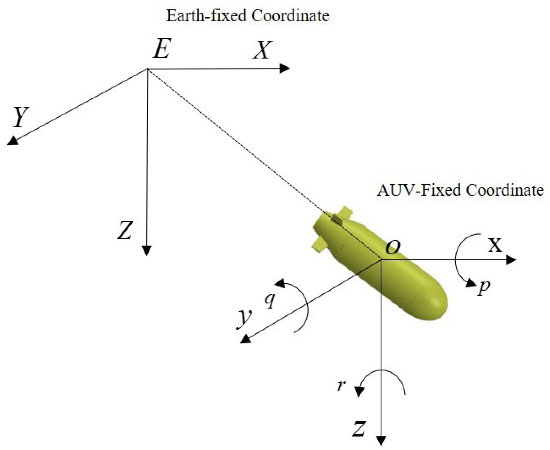
2. AUV Kinematic and Dynamic Models

According to the AUV motion properties and neglecting the roll dynamics, the 5-degree-of-freedom (DOF) kinematic and dynamics models of an underactuated AUV can be expressed as [24]:

$$\begin{array}{cc}\hfill \dot{x}& =ucos\left(\theta \right)cos\left(\psi \right)-vsin\left(\psi \right)+wsin\left(\theta \right)cos\left(\psi \right),\hfill \\ \hfill \dot{y}& =ucos\left(\theta \right)sin\left(\psi \right)+vcos\left(\psi \right)+wsin\left(\theta \right)sin\left(\psi \right),\hfill \\ \hfill \dot{z}& =-usin\left(\theta \right)+wcos\left(\theta \right),\hfill \\ \hfill \dot{\theta }& =q,\hfill \\ \hfill \dot{\psi }& =r/cos\left(\theta \right),\hfill \end{array}$$

(1)

$$\begin{array}{cc}\hfill \dot{u}& =\frac{m_{22}}{m_{11}}vr-\frac{m_{33}}{m_{11}}wq-\frac{d_{11}}{m_{11}}u+\frac{1}{m_{11}}{\tau }_u,\hfill \\ \hfill \dot{v}& =-\frac{m_{11}}{m_{22}}ur-\frac{d_{22}}{m_{22}}u,\hfill \\ \hfill \dot{w}& =\frac{m_{11}}{m_{33}}uq-\frac{d_{33}}{m_{33}}w,\hfill \\ \hfill \dot{q}& =\frac{m_{33}-m_{11}}{m_{55}}uw-\frac{d_{55}}{m_{55}}q-\frac{\rho g▽G{M}_{L}sin\left(\theta \right)}{m_{55}}+\frac{1}{m_{55}}{\tau }_q,\hfill \\ \hfill \dot{r}& =\frac{m_{11}-m_{22}}{m_{66}}uv-\frac{d_{66}}{m_{66}}r+\frac{1}{m_{66}}{\tau }_r,\hfill \end{array}$$

(2)

where x, y, z, $\theta$ and $\psi$ are the positions and attitude of the AUV in the earth-fixed frame in Figure 1; u, v, w, q and r are the corresponding linear and angular velocities in the body-fixed frame; ${\tau }_u$, ${\tau }_q$ and ${\tau }_r$ are the control forces and moments of the AUV produced by thrusters and propellers; $m_{ii}$ ($i=1,2,3,5,6$) denote the inertia and added mass parameters of the AUV, and $d_{ii}$$(i=1,2,3,5,6$) denote the hydrodynamic damping coefficients, ∇ denotes the volume of fluid displaced by the AUV, g denotes the acceleration of gravity, $\rho$ denotes the fluid density, G denotes the gravity of the AUV, and $M_L$ denotes the distance between the center of gravity and the center of buoyancy [25].

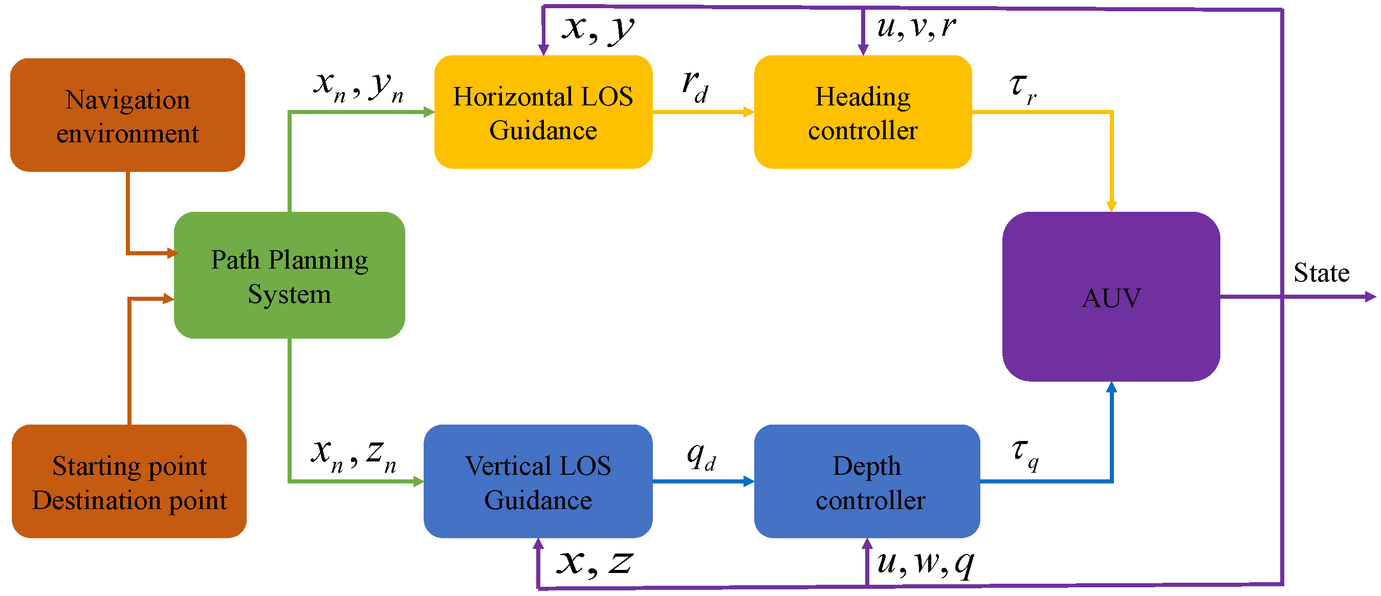
3. Three-Dimensional Guidance System

The 3D guidance system is motivated by the 2D guidance law. This paper simplifies a 3D guidance system into two independent and decoupled 3-DOF cases; namely, the horizontal-plane guidance and the vertical-plane guidance. The horizontal-plane guidance strategy makes AUVs converge to a straight line on the horizontal plane via generating the reference heading angle; similarly, the vertical-plane guidance strategy generates the reference pitch angle to converge to a straight line on the vertical plane. The block diagram of the 3D guidance system is given in Figure 2.

To obtain the 3D guidance algorithm, the original 2D guidance algorithm is extended. The inertial frame is transformed into the path frame by two rotations, and the tracking error vector is built to clearly represent the distance from the AUV to the path.

The first step is to rotate the inertial frame by $\alpha$ around the z axis, and the second step is to rotate the resulting frame from the first rotation by $\beta$ around the y axis, where $\alpha$ and $\beta$, defined by (3) and (4), are the slope of the trajectory straight line before each rotation. The rotations can be described by two rotation matrices, ${\mathit{R}}_z\left(\alpha \right)$ and ${\mathit{R}}_y\left(\beta \right)$, given in (5) and (6), respectively.

$$\begin{array}{ccc}\hfill \alpha & =\hfill & \hfill arctan\left(\frac{y_{i+1}-y_i}{x_{i+1}-x_i}\right),\end{array}$$

(3)

$$\begin{array}{ccc}\hfill \beta & =\hfill & \hfill arctan\left(\frac{z_i-z_{i+1}}{\sqrt{{(x_{i+1}-x_i)}^2+{(y_{i+1}-y_i)}^2}}\right),\end{array}$$

(4)

$$\begin{array}{cc}\hfill {\mathit{R}}_z\left(\alpha \right)& =\left(\begin{array}{ccc}cos\left(\alpha \right)& sin\left(\alpha \right)& 0\\ -sin\left(\alpha \right)& cos\left(\alpha \right)& 0\\ 0& 0& 1\end{array}\right),\hfill \end{array}$$

(5)

$$\begin{array}{cc}\hfill {\mathit{R}}_y\left(\beta \right)& =\left(\begin{array}{ccc}cos\left(\beta \right)& 0& -sin\left(\beta \right)\\ 0& 1& 0\\ sin\left(\beta \right)& 0& cos\left(\beta \right)\end{array}\right).\hfill \end{array}$$

(6)

Then, the tracking error vector $\mathit{e}={[e_x,e_y,e_z]}^T$ can be computed in the path frame as (7), where $e_x$, $e_y$ and $e_z$ are the along, cross and vertical tracking errors, respectively.

$$\begin{array}{cc}\hfill \mathit{e}& ={\mathit{R}}_y\left(\beta \right){\mathit{R}}_z\left(\alpha \right)(\mathit{p}-{\mathit{W}}_i).\hfill \end{array}$$

(7)

In order to make the AUV follow the desired path, the lookahead guidance algorithm is employed by introducing a virtual target [26]. In this algorithm, the error components $e_y$ and $e_z$ are used to guide the AUV to the virtual target. To guarantee that the tracking errors $e_y$ and $e_z$ converge to zero, the guidance angles ${\psi }_d$ and ${\theta }_d$ are set as

$$\begin{array}{ccc}\hfill {\psi }_d& =\hfill & \hfill \alpha +arctan\left(\frac{-e_y}{{\delta }_y}\right),\end{array}$$

(8)

$$\begin{array}{ccc}\hfill {\theta }_d& =\hfill & \hfill \theta +arctan\left(\frac{e_z}{{\delta }_z}\right).\end{array}$$

(9)

where ${\delta }_y$ and ${\delta }_z$ are designed to force the position of the AUV to the $xz$ and $xy$ planes of the path frame, respectively. Then, we can obtain the desired angular velocities $q_d$ and $r_d$ by proportional controller gains $k_{\psi }$ and $k_{\theta }$.

The steps of the lookahead guidance algorithm for AUVs are listed in Algorithm 1.

Algorithm 1: Lookahead guidance algorithm.

Input:$({\mathit{W}}_i={[x_i,y_i,z_i]}^T,{\mathit{W}}_{i+1}={[x_{i+1},y_{i+1},z_{i+1}]}^T,\mathit{p}={[x,y,z]}^t,\psi ,\theta ,{\delta }_y,{\delta }_z,k_{\psi },k_{\theta },i=(1,2\cdots ,n))$ Output:$(r_d,q_d)$ 1: for$i=1$ to $n-1$ do 2:     $\alpha \leftarrow arctan\left(\frac{y_{i+1}-y_i}{x_{i+1}-x_i}\right)$ 3:     ${\mathit{W}}_i^R={\mathit{R}}_z\left(\alpha \right){\mathit{W}}_i$ 4:     $⊳{\mathit{W}}_i^R={[x_i^R,y_i^R,z_i^R]}^T$ 5:     ${\mathit{W}}_{i+1}^R\leftarrow {\mathit{R}}_z\left(\alpha \right){\mathit{W}}_{i+1}$ 6:     $\beta \leftarrow arctan\left(\frac{z_i^R-z_{i+1}^R}{x_{i+1}^R-x_i^R}\right)$ 7:     $⊳\mathit{e}={[e_x,e_y,e_z]}^T$ 8:     $\mathit{e}={\mathit{R}}_y\left(\beta \right){\mathit{R}}_z\left(\alpha \right)(\mathit{p}-{\mathit{W}}_i)$ 9:     ${\psi }_d=\alpha +arctan\left(\frac{-e_y}{{\delta }_y}\right)$ 10:    ${\theta }_d=\theta +arctan\left(\frac{e_z}{{\delta }_z}\right)$ 11:    $r_d=k_{\psi }({\psi }_d-\psi )$ 12:    $q_d=k_{\theta }({\theta }_d-\theta )$ 13:    return $(r_d,q_d)$

This paper designs two independent controllers for the underactuated AUV based on the desired surge velocity $u_d$, the desired pitch angle rate $q_d$, and the desired heading angle rate $r_d$ to control the horizontal-plane and vertical-plane motions, respectively [27].

Define the surge velocity error $z_1$, the pitch angle rate error $z_2$ and the heading angle rate error $z_3$ as:

$$\begin{array}{cc}\hfill z_1:& =u-u_d,\hfill \\ \hfill z_2:& =q-q_d,\hfill \\ \hfill z_3:& =r-r_d.\hfill \end{array}$$

(10)

Step 1: Differentiating (10) with respect to time, respectively, and we have

$$\begin{array}{cc}\hfill m_{11}{\dot{z}}_1& =m_{11}\dot{u}-m_{11}\dot{u_d},\hfill \\ \hfill m_{55}{\dot{z}}_2& =m_{55}\dot{q}-m_{55}{\dot{q}}_d,\hfill \\ \hfill m_{66}{\dot{z}}_3& =m_{66}\dot{r}-m_{66}{\dot{r}}_d.\hfill \end{array}$$

(11)

Step 2: The control law can be designed as:

$$\begin{array}{cc}\hfill {\tau }_u& =-k_1{z}_1-m_{22}vr+m_{33}wq+d_{11}u+m_{11}\dot{u_d},\hfill \\ \hfill {\tau }_q& =-k_2{z}_2-(m_{33}-m_{11})uw+d_{55}q+(\rho g▽G{M}_{L}sin\left(\theta \right))+m_{55}{\dot{q}}_d,\hfill \\ \hfill {\tau }_r& =-k_3{z}_3-(m_{11}-m_{22})uv+d_{66}r+m_{66}{\dot{r}}_d,\hfill \end{array}$$

(12)

where $k_1>0$, $k_2>0$ and $k_3>0$ are the parameters to be designed.

Step 3: Define a Lyapunov function candidate as:

$$\begin{array}{cc}\hfill V(z_1,z_2,z_3)& =\frac{1}{2}{m}_{11}{z_1}^2+\frac{1}{2}{m}_{55}{z_2}^2+\frac{1}{2}{m}_{66}{z_3}^2.\hfill \end{array}$$

(13)

Differentiating the Lyapunov function with respect to time, and we have

$$\begin{array}{cc}\hfill \dot{V}(z_1,z_2,z_3)& =z_1{m}_{11}{\dot{z}}_1+z_2{m}_{55}{\dot{z}}_2+z_3{m}_{66}{\dot{z}}_3.\hfill \end{array}$$

(14)

Substituting Equations (2), (11) and (12) into (15), and we have

$$\begin{array}{cc}\hfill \dot{V}(z_1,z_2,z_3)& =z_1{m}_{11}{\dot{z}}_1+z_2{m}_{55}{\dot{z}}_2+z_3{m}_{66}{\dot{z}}_3\hfill \\ \hfill & =z_1{m}_{55}(\dot{u}-\dot{u_d})+z_2{m}_{55}(\dot{q}-{\dot{q}}_d)+z_3{m}_{66}(\dot{r}-{\dot{r}}_d)\hfill \\ \hfill & =-k_1{z_1}^2-k_2{z_2}^2-k_3{z_3}^2\le 0.\hfill \end{array}$$

(15)

According to the Lyapunov stability theorem, the errors $z_1$, $z_2$ and $z_3$ can converge to zero, and the closed-loop system is asymptotically stable.

4. Multi-Objective Optimization

If ${\mathit{P}}_0$ is the starting point and ${\mathit{P}}_N$ is the destination point, then the path can be expressed as follows:

$$\begin{array}{cc}\hfill \mathit{W}& =({\mathit{P}}_0,x_1,y_1,z_1,\dots ,x_n,y_n,z_n,{\mathbf{P}}_N),\hfill \end{array}$$

(16)

where ${\mathit{P}}_n=(x_n,y_n,z_n)$ is a middle waypoint of the path, both the line segment from $(x_{n-1},y_{n-1},z_{n-1})$ to $(x_n,y_n,z_n)$ and the line segment from $(x_n,y_n,z_n)$ to $(x_{n+1},y_{n+1},z_{n+1})$ do not cut obstacle areas.

According to the given navigation environment and the physical property of AUVs, some formal constraints are formulated as follows:

$$\begin{array}{ccc}\hfill x_{min}& <x_n<x_{max},\hfill & \hfill n=\overline{1,n},\\ \hfill y_{min}& <y_n<y_{max},\hfill & \hfill n=\overline{1,n},\\ \hfill z_{min}& <z_n<z_{max},\hfill & \hfill n=\overline{1,n},\\ \hfill \gamma & <{\gamma }_{max},\hfill \\ \hfill \phi & >{\phi }_{min},\hfill \end{array}$$

(17)

where $x_{min}$ and $x_{max}$ are constraints for $x_n$, $y_{min}$ and $y_{max}$ are constraints for $y_n$, $z_{min}$ and $z_{max}$ are constraints for $z_n$, ${\gamma }_{max}$ is the maximum allowed angle of the planning path on the horizontal plane, and ${\phi }_{min}$ is the minimal allowed angle of the planning path on the vertical plane.

4.1. Path Length

The total length of the path is usually discussed because it determines the sailing time and energy expenditure. The total length of the path can be calculated by:

$$\begin{array}{cc}\hfill L& =\sum _{n=1}^N\parallel {\mathit{P}}_n-{\mathit{P}}_{n-1}\parallel ,\hfill \end{array}$$

(18)

where $\parallel {\mathit{P}}_n-{\mathit{P}}_{n-1}\parallel$ indicates the Euclidean distance between ${\mathit{P}}_n=(x_n,y_n,z_n)$ and ${\mathit{P}}_{n-1}=(x_{n-1},y_{n-1},z_{n-1})$.

During path planning, the path length ratio is usually used to calculate the path length, specifically as follows:

$$\begin{array}{cc}\hfill A_1& =\frac{L}{\parallel {\mathit{P}}_N-{\mathit{P}}_0\parallel },\hfill \end{array}$$

(19)

where $\parallel {\mathit{P}}_N-{\mathit{P}}_0\parallel$ represents the Euclidean distance between the starting point ${\mathit{P}}_0$ and the destination point ${\mathit{P}}_N$.

4.2. Path Smoothness

Path smoothness should be considered to avoid the mutations in navigation direction in path planning. Mutations in navigation direction will not only increase energy consumption, but also reduce navigation accuracy. Therefore, in order to avoid the mutations in navigation direction, the fitness function is defined as:

$$\begin{array}{cc}\hfill A_2& =\sum _{n=1}^N\frac{{\gamma }_n}{min(\parallel (x_{n-1},y_{n-1}),(x_n,y_n)\parallel ,\parallel (x_n,y_n),(x_{n+1},y_{n+1})\parallel )}\hfill \\ \hfill & +\sum _{n=1}^N\frac{{\phi }_n}{\sqrt{{(z_n-z_{n-1})}^2+\left({(x_n-x_{n-1})}^2\right)}},\hfill \end{array}$$

(20)

where $\parallel ·\parallel$ represents the Euclidean distance, ${\gamma }_n$ and ${\phi }_n$ represent the angle of the planning path on the horizontal plane and the angle of the planning path on the vertical plane, which are calculated according to the following formula:

$$\begin{array}{cc}\hfill {\gamma }_n& =\left|arctan\left[\frac{z_n-z_{n-1}}{\sqrt{{(x_n-x_{n-1})}^2+{(y_n-y_{n-1})}^2}}\right]\right|,\hfill \\ \hfill {\phi }_n& =\pi -\left|arccos\left[\frac{(x_n-x_{n-1})(x_{n+1}-x_n)+(y_n-y_{n-1})(y_{n+1}-y_n)}{\sqrt{{(x_n-x_{n-1})}^2+{(y_n-y_{n-1})}^2}+\sqrt{{(x_{n+1}-x_n)}^2+{(y_{n+1}-y_n)}^2}}\right]\right|.\hfill \end{array}$$

(21)

4.3. Path Safety

A safe path must avoid all the obstacles. The obstacles are assumed to be static with known position. The underwater obstacle is usually assumed to be a stationary target and positioned. The solutions should be penalized when the generated path cuts any obstacles. The safety fitness function of the path can be expressed as:

$$\begin{array}{c}\hfill A_3=\left\{\begin{array}{cc}\hfill +\infty ,& \mathrm{if}{\mathit{P}}_n{\mathit{P}}_{n-1}\bigcap OB\ne \varnothing ,\hfill \\ \hfill 0,& \mathrm{if}{\mathit{P}}_n{\mathit{P}}_{n-1}\bigcap OB=\varnothing ,\hfill \end{array}\right.\end{array}$$

(22)

where $A_3$ is the fitness function of the path, $OB$ represents the collection of all obstacle areas, if the planned path does not intersect all obstacles, the fitness function of the path is 0, conversely, it is $+\infty$.

4.4. The Construction of the Total Fitness Function

The path planning algorithm takes the path length, the path safety and the path smoothness as the main optimization goal. It is common to aggregate the multiple objectives into a single fitness function, which is nonzero and monotonic. The total fitness function of the path comes from a weighted sum of objectives above, and the smaller fitness function value represents a better path. Define the total fitness function as:

$$\begin{array}{cc}\hfill & F={\eta }_1{A}_1+{\eta }_2{A}_2+{\eta }_3{A}_3,\hfill \\ \hfill & \sum _{i=1}^{}{\eta }_i=1,\hfill \end{array}$$

(23)

where F represents the total fitness function of the path, ${\eta }_i$ (i = 1, 2, 3) are weight factors that determine the importance of each objective.

5. The Improved SPSO-2011 Algorithm

Evolutionary algorithms have been widely applied to solve multi-objective optimization engineering problems. One of the most popular evolutionary algorithms is the particle swarm optimization (PSO) algorithm.

The SPSO-2011 exploits the idea of rotational invariance to improve the standard PSO. The improved SPSO-2011 algorithm still utilizes the update rules of the SPSO-2011 algorithm and uses the uniform random initialization. Velocity and position of the particle are updated by

$$\begin{array}{cc}\hfill {\mathit{V}}_i(t+1)& =\omega {\mathit{V}}_i\left(t\right)-\frac{c1+c2}{3}{\mathit{X}}_i\left(t\right)+\frac{c1{\mathit{P}}_{bes{t}_i}\left(t\right)+c2{\mathit{G}}_{best}}{3},\hfill \\ \hfill {\mathit{X}}_i(t+1)& ={\mathit{X}}_i\left(t\right)+{\mathit{V}}_i(t+1),\hfill \end{array}$$

(24)

where $i=1,2,\cdots ,M$, with M equal to swarm size and $t=1,2,\cdots ,T$ with T equal to the maximum number of iterations, $\mathit{V}$ represents the velocity of the particle, $\mathit{X}$ the position of the particle, $\omega$ is the inertia weight, $c1$ is the cognitive learning factor, $c2$ is the social learning factor, ${\mathit{G}}_{best}$ denotes the best position that the whole swarm has found so far, and ${\mathit{P}}_{best}$ denotes the best position that the particle has found so far.

5.1. The Improved Adaptive Parameters

The inertia weight $\omega$ is applied to balance the global and local search capabilities. The larger the w, the faster the particle convergence rate and the stronger the global search ability, but it reduces the local search ability of the particles and ultimately leads to lower global convergence accuracy. The smaller w will improve the convergence accuracy of the particles, but reduces the convergence speed of the particles, which easily makes the particle into the local optimum in the search process and cannot jump out of the local extreme value [28]. In the SPSO-2011 algorithm, the inertia weight is a fixed value, but it cannot consider both the search accuracy and the search range. A nonlinear adaptive strategy can ensure that all particles can quickly spread into the whole search space in the early search stage to determine the approximate range of the global extrema, accelerating the particle convergence in the late search stage [29]. In the improved SPSO-2011 algorithm, the inertia weight w linearly increases in the early stage, which increases the search range, prevents falling into the local optimum, and then the inertia weight w nonlinearly reduces in the late stage to improve the search accuracy. The nonlinear adaptive inertia weight was proposed as the followed formula:

$$\begin{array}{cc}\hfill \omega & ={\omega }_r+(\frac{t}{T})*({\omega }_{max}-{\omega }_{min}),0<t<\frac{T-ite{r}_{min}}{2},\hfill \\ \hfill \omega & ={\omega }_{min}+e^{\frac{-{(k*t)}^2}{T}}*({\omega }_{max}-{\omega }_{min}),\frac{T-ite{r}_{min}}{2}<t<T,\hfill \\ \hfill \omega & ={\omega }_{max},\omega >{\omega }_{max},\hfill \end{array}$$

(25)

where ${\omega }_r$ represents the initial value, ${\omega }_{min}$ is the minimum value, ${\omega }_{max}$ is the maximum value, and $ite{r}_{min}$ represents the minimum number of iterations.

In the SPSO-2011 algorithm, the update speed of the particle swarm is mainly adjusted through the cognitive learning factor and the social learning factor, but due to the lack of changes in learning factors, it is easy to make the particle fall into the local optimum. In the improved SPSO-2011 algorithm, two learning factors are devised with dynamic adjustment methods to avoid the local optimum. The dynamic adjustment methods are as follows:

$$\begin{array}{cc}\hfill c1& =c{1}_{max}-K_1*\frac{t}{T}*(c{1}_{max}-c{1}_{min}),\hfill \\ \hfill c2& =c{2}_{min}+K_2*\frac{t}{T}*(c{2}_{max}-c{2}_{min}),\hfill \end{array}$$

(26)

where $c{1}_{min}$ represents the minimum value of the cognitive learning factor, $c{2}_{min}$ represents the minimum value of the social learning factor, $c{1}_{max}$ represents the maximum value of the cognitive learning factor, $c{2}_{max}$ represents the maximum value of the social learning factor, and $K_1$ and $K_2$ represent two adjustable and positive constants.

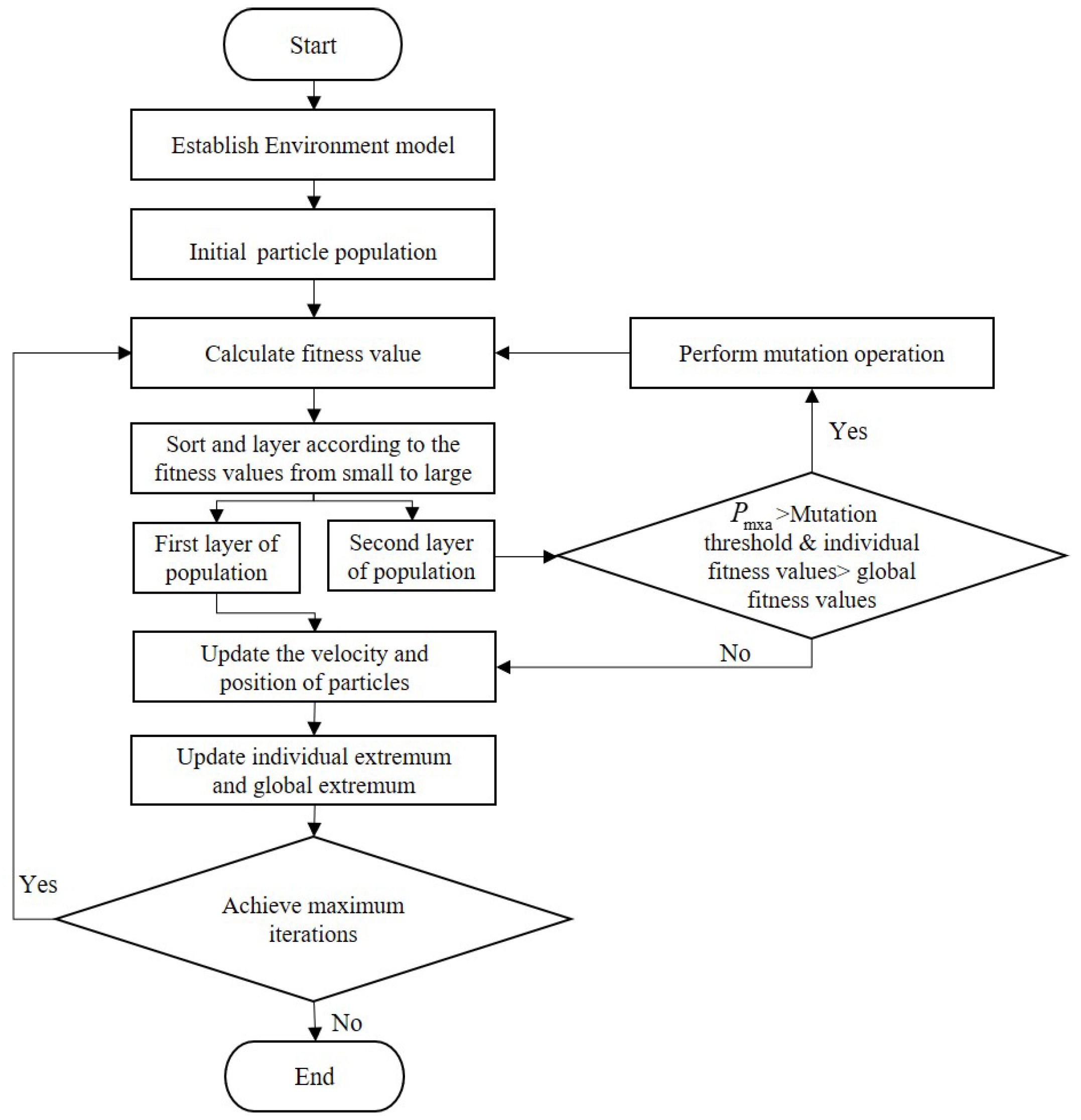
5.2. Mutation Operator

The mutation is employed to give new information to the population and increase population diversity. In this paper, the improved SPSO-2011 algorithm introduces a mutation operator with a threshold. In the improved SPSO-2011 algorithm, when the cumulative number of iterations is greater than the threshold and the individual fitness function value is always greater than the global fitness function in the cumulative process, the mutation is performed. Otherwise, the cumulative number of iterations is 0. The improved method can effectively increase global search ability and avoid falling into the local optimum. The random mutation can be expressed by the following equation:

$$\begin{array}{cc}\hfill X_i(t+1)& =rand*D,\hfill \end{array}$$

(27)

where $rand$ is the random number in the $[0,1]$ and D is the range of map.

The flow chart of the improved SPSO-2011 algorithm is shown in Figure 3.

6. Simulation Results

To verify the effectiveness of the proposed algorithm, this paper contrasts with the PSO and SPSO-2011 algorithms in terms of planning time and path length. For certain AUV, a 3D guidance and control strategy is designed, and a closed-loop simulation system is established based on MATLAB/Simulink. Comparative simulations are carried out to verify the effectiveness of the proposed algorithm.

The simulations are carried out in different 3D spaces with different obstacles and different starting and destination points. In general, the underwater obstacles mainly include sea ridges, underwater shipwrecks, marine suspended matter and other objects. To facilitate the problem description, the sphere and cuboids are used to describe the underwater obstacles. The parameters of the proposed Improved SPSO-2011 algorithm are given in

Table 1. The parameters of the improved SPSO-2011 algorithm.

Variables	Value
${\gamma }_{max}$	$\pi /3$
${\phi }_{min}$	$\pi /6$
${\omega }_r$	$0.7$
${\omega }_{min}$	$0.4$
${\omega }_{max}$	$0.9$
$ite{r}_{min}$	70
$c{1}_{min}$	$0.9$
$c{2}_{min}$	$0.9$
$c{1}_{max}$	$2.1$
$c{2}_{max}$	$2.1$
$P_{max}$	7
$K_1$	$0.2$
$K_2$	$0.2$
M	200
T	100
k	$1.5$

. The simulations are carried out on a 500 m × 500 m × 100 m 3D space with some equivalent obstacles. In 3D space, the starting point is $(2,10,7)$, and the destination point is $(480,430,30)$. All obstacles are replaced by regular balls or cuboids. The main parameters of the improved SPSO-2011 algorithm are: ${\gamma }_{max}<|\pm \pi /3|$, ${\phi }_{min}>|\pm \pi /6|$, $M=200$, ${\omega }_r=0.7$, ${\omega }_{min}=0.4$, ${\omega }_{max}=0.9$, $c{1}_{min}=c{2}_{min}=0.9$, $c{1}_{max}=c{2}_{max}=2.2$, $K_1=K_2=0.2$, $ite{r}_{min}=70$, $T=100$, $k=1.5$ and $P_{max}=7$. Model parameters of the AUV are given by $m_{11}=25$ kg, $m_{22}=17.5$ kg, $m_{33}=30$ kg, $m_{55}=22.5$ kgm${}^2$, $m_{66}=15$ kgm${}^2$, $d_{11}=30$ kgs${}^{-1}$, $d_{22}=30$ kgs${}^{-1}$, $d_{33}=30$ kgs${}^{-1}$, $d_{55}=25$ kgm${}^2$s${}^{-1}$, $d_{66}=25$ kgm${}^2$s${}^{-1}$, and $\rho g\nabla G{M}_L=5$[30,31]. The initial states of the AUV are set as $\left[x\right(0),y(0),z(0),\theta (0),\psi (0\left)\right]=\left[2\right(m),10(m),7(m),0(rad),0(rad\left)\right]$. The constant surge velocity of the AUV is set as $u_d$ = 1.5 ms${}^{-1}$. The 3D guidance algorithm and controller parameters are chosen as $k_1=1$, $k_2=1$, $k_3=1$, $k_{\psi }=1$, $k_{\theta }=1$, ${\delta }_y=10$ and ${\delta }_z=10$.

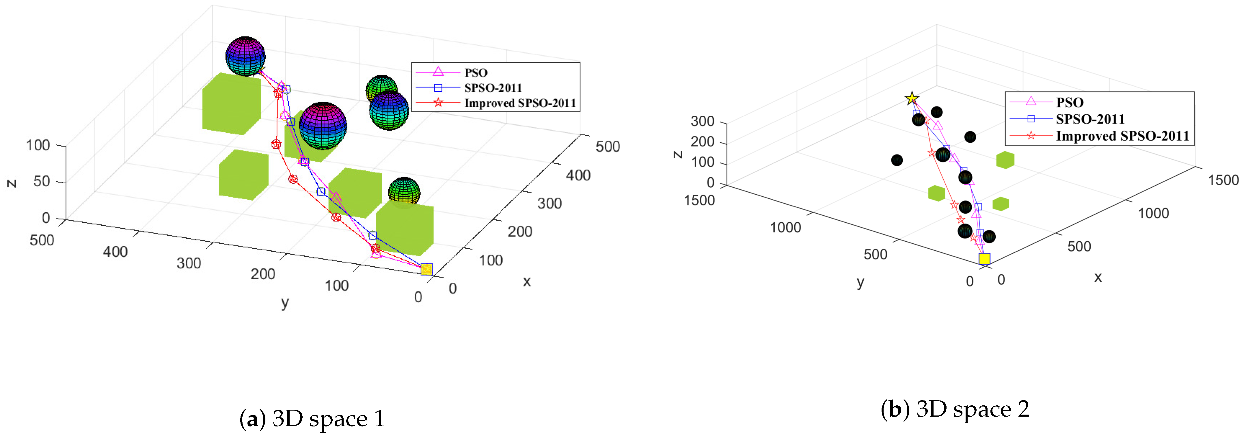
The parameters of 3D space and the positions of starting and destination points are shown in

Table 2. Performance comparisons of path planning algorithms in different 3D spaces.

Algorithm	3D Spaces	The Shortest Distance of Paths (Meters)	The Average Distance of Paths (Meters)
PSO	3D space1: 500 m × 500 m × 100 m	663.54	665.98
SPSO-2011	The starting point: $(2,10,7)$	660.10	669.99
Improved SPSO-2011	The destination point: $(480,430,30)$	655.12	657.26
PSO	3D space2: 1500 m × 1500 m × 300 m	1828.35	1834.77
SPSO-2011	The starting point: $(18,20,25)$	1829.83	1836.91
Improved SPSO-2011	The destination point: $(1200,1400,60)$	1820.89	1827.71

. Simulations of the PSO algorithm, the SPSO-2011 algorithm and the improved SPSO-2011 algorithm are performed using MATLAB, and each three path planning algorithms were performed eight times. The optimal fitness function values of three path planning algorithms in different 3D spaces with different obstacles and different starting and destination points are shown in Figure 4. It can be clearly observed that the proposed improved SPSO-2011 algorithm has a faster convergence rate and the minimum fitness function values 0.9145 and 0.8926 for 3D space 1 and 2, respectively. This confirms that the proposed improved SPSO-2011 algorithm has better performance than the PSO and SPSO-2011 algorithms. The optimal planned paths of three path planning algorithms are shown in Figure 5. The shortest distance of the paths, and the average distance of the paths of three path planning algorithms, are shown in Table 2. As seen in Figure 5 and Table 2, under the proposed improved SPSO-2011 algorithm, the planned path has the shorter path length and higher path smoothness in 3D spaces 1 and 2. From the values of the average distance of the paths in Table 2, the proposed algorithm has the shortest average distance of the paths, and thus can effectively avoid falling into the local optimum.

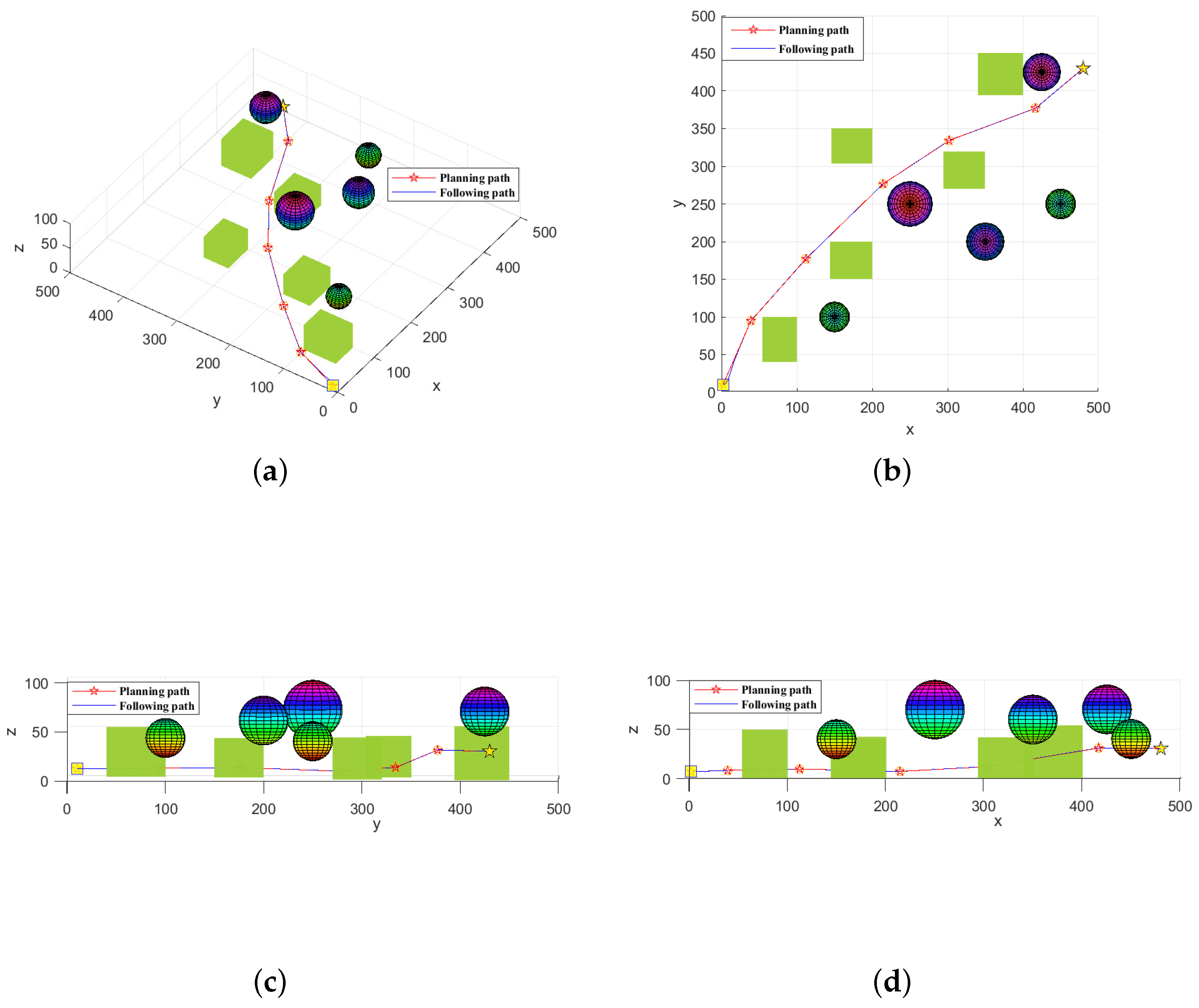
To verify the path performability, the planned path in the 3D space 1 is selected for tracking control by employing the proposed 3D guidance and control algorithm. The simulation results are illustrated in Figure 6 and Figure 7. The 3D following trajectory of the AUV is illustrated in Figure 6a. The corresponding following trajectories in the xy, xz and yz planes are illustrated in Figure 6b–d, respectively. 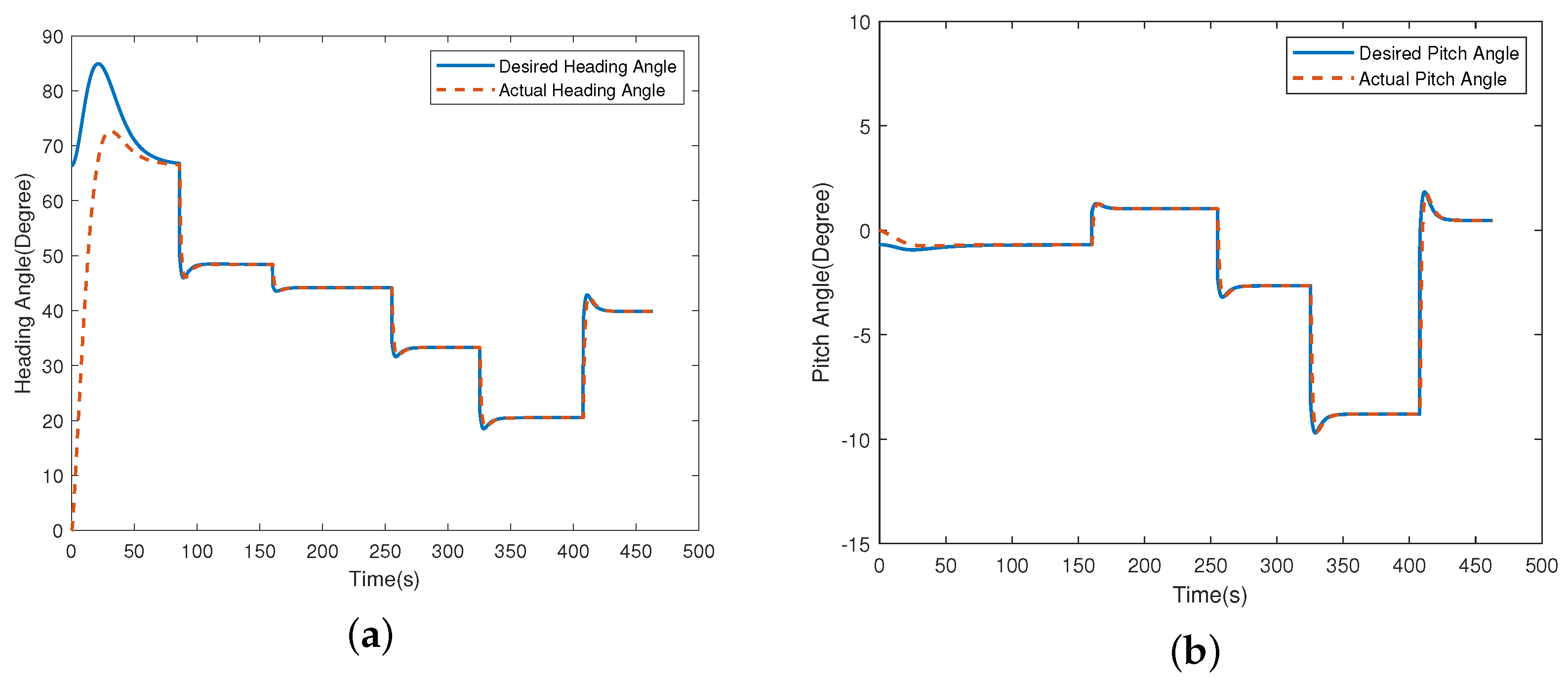Figure 7a shows the desired heading angle and actual heading angle. Figure 7b shows the desired pitch angle and actual pitch angle. From Figure 6 and Figure 7, we can observe that the proposed 3D guidance and control algorithm can make the AUV track the planned path accurately and the desired heading and pitch angles are reasonable.

Simulation results demonstrate the effectiveness of the proposed algorithm. Compared with the PSO algorithm and SPSO-2011 algorithm, the proposed algorithm has the following advantages:

• Under the proposed algorithm, the phenomenon of local optima can be avoided effectively and thus plan shorter path lengths.
• The proposed algorithm has the faster convergence rate and higher accuracy.
• The proposed 3D guidance algorithm can accurately track the planned path, indicating that the planned path has good performability.

7. Conclusions

This paper proposes an improved SPSO-2011 algorithm. A mutation operator with a threshold is introduced to prevent falling into local optima and a nonlinear adaptive parameter strategy is introduced to accelerate convergence speed. The construction of the total fitness function considers “path length”, “path smoothness”, “path safety” and “physical constraints”, which can effectively avoid collision with threats, obtain a shorter path, and save energy consumption. Compared with the PSO algorithm and the SPSO-2011 algorithm, simulation results show that the proposed algorithm has greater advantages in terms of path length and planning time. To verify the performability of the planned path, a 3D guidance algorithm and controller are designed for AUVs. Simulation results show that the AUV can accurately track the planned path based on the improved SPSO-2011 algorithm.