Improved Fractional-Order PID Controller of a PMSM-Based Wave Compensation System for Offshore Ship Cranes

Abstract

Wave compensation technology is crucial to the safety of the ship operation and the accurate placement of load. Its compensation efficiency and the gentle change of the rope tension are particularly important. In this paper, we adopt permanent magnet synchronous machine (PMSM) as the actuator to construct the basic wave compensation system. Firstly, the motion model of ship and load under wave action is established, and the fractional-order PID (FOPID) controller for the position loop of the PMSM is introduced. Then, the parameters of FOPID are optimized by genetic algorithm-particle swarm optimization (GAPSO) algorithm, which is based on genetic algorithms (GA) and particle swarm optimization (PSO) algorithms for better compensation performance. The wave synchronization strategy is used to simulate the load, when it needs to be taken into the water. The non-linear dynamic equations of the rope are solved by Lagrange mechanics and the heave displacement is obtained by time series prediction algorithm. Finally, the effect of wave compensation and wave synchronization strategy are verified on MATLAB/Simulink. The results show that after the compensation, the crane load can follow the set height value very well, the compensation efficiency can reach more than 94%, and the wave synchronization strategy significantly reduces the change of the rope tension.

1. Introduction

The offshore oil and gas industry includes activities related to the exploration, extraction, transportation, and processing of offshore oil and gas. With the depletion of onshore oil and gas resources, exploration and development of offshore oil and gas has become an important strategy for many countries and regions. Consequently, the safety of marine operations above the sea surface and the safety oil and gas operations below the sea surface is a key feature [1,2].

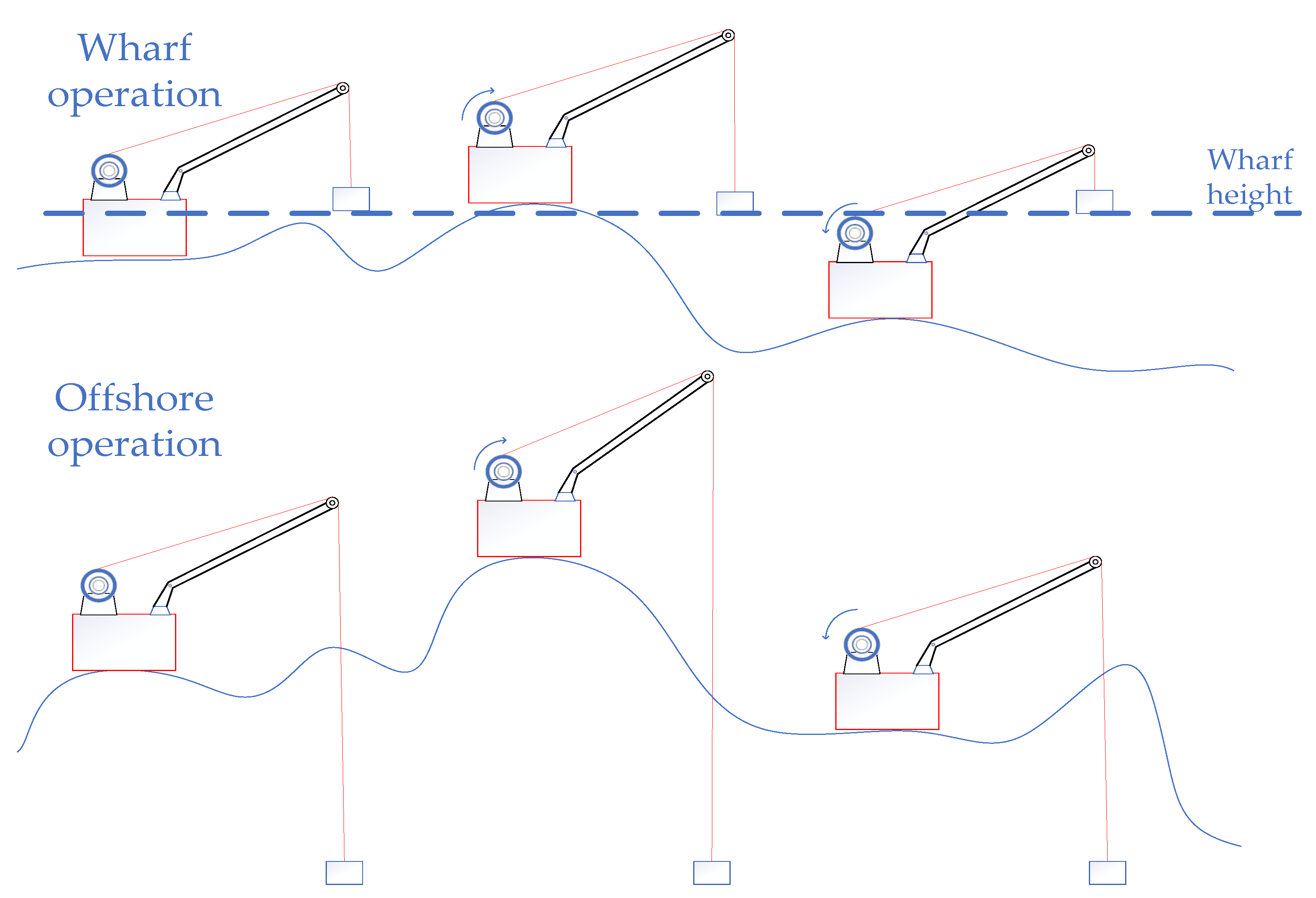
When the vessel is disturbed by wind and waves, 6 degrees of freedom (DOF) motion will make the crane load deviate from its desired position. This phenomenon will highly affect the system’s controllability and lead to system damage. In the 6 DOF motion, the heave motion has the most significant impact on the load when the vessel crane is lifting objects at the wharf or offshore. Consequently, when the vessel rises and falls with the waves, in order to keep the load at the set position, as shown in Figure 1, the vessel heave compensation system is particularly important. The current heave compensation systems are mainly divided into two categories: a passive compensation system (PCS) and an active compensation system (ACS) [3].

Although PCS is relatively simple in structural design, there are still many shortcomings: PCS does not have a closed loop, which makes feedback control impossible; PCS also has a large delay, which brings a lag in compensation effects [4]. PCSs use only mechanical equipment for buffering and has an efficiency less than 80%. If higher compensation efficiency and accuracy is desired, the use of ACS is needed [5]. Generally, the compensation efficiency of ACS can reach more than 90%. Compared with PCS, it has a better timely compensation performance, better regulation ability for over-compensation, and can drastically reduce the heave motion of the load coupling.

In 1970, A. Southerland designed a hybrid heave compensation system: a passive system to maintain constant rope tension and an active system to control the heave motion [6]. Later, developments in the oil and gas industry led to further research into heave compensation systems. A circuit system was proposed to compensate for gravitational movement, but due to the limitations of the technology at the time, this circuit structure could not be changed once the design was completed. Another limitation was linked to the fact that the accuracy of the measurement system was low. To ensure the accuracy of the system, the use of a more expensive inertial measurement unit (IMU) to measure the vessel’s motion is needed. A GPS-based measurement scheme that can reduce costs has therefore been proposed instead, using a GPS comparable to the IMU but with a limited sampling frequency.

To cope with the disturbance of wind and waves, assorted control strategies have been proposed for the actuator. Pan et al. explored a Lyapunov’s direct method based nonlinear control strategy to adjust the distance from the upper end of the riser to the seabed to reduce the effect of the heave motion of the vessel [7]. Johansen et al. introduced wave synchronization for active control strategy to use a wave-amplitude measurement to minimize variation in the relative vertical velocity between the load and water. The results indicated that the reduction in the standard deviation of the rope tension may be up to 50% [8]. Yan et al. designed an adaptive robust integral sliding mode control (ARISMC) based on the back-stepping control method strategy to realize constant tension control of hybrid active-passive heave compensator (HAHC) applied to heavy deep-sea towing systems [9]. Sandre-Hernandez et al. introduced a PSO algorithm to identify the direct and quadrature stator inductances and the stator resistance of a PMS compensation motor [10], nevertheless, PSO algorithm is prone to find local optima when dealing with parameter optimization.

For the typical three-loop control of the compensation PMSM, Sun et al. proposed an improved model predictive current control (MPCC) scheme to select the optimal voltage vector based on a current track circle instead of a cost function to improve the steady state and dynamic performance [11]. Gao et al. proposed a new single-loop model predictive control (MPC) based on back-electromotive force and I-F control to simplify the system structure and control algorithm. It has a high dynamic and steady-state performance [12]. Zhang et al. designed an asymmetric space vector modulation (ASVM) method to improve the calculated position estimate [13]. Liu et al. proposed a closed-loop detection system to accurately extract harmonics and to use a compensation algorithm to suppress harmonics in winding currents [14].

The paper’s main contributions to address the previously presented issues are the following:

To accurately obtain the load motion information, this paper solves the non-linear dynamic equations of the rope by using the Lagrange mechanics principle, and the length of the rope is thought to be variable.

To solve the traditional FOPID parameter adjustment difficulties, this paper introduces the GAPSO algorithm to optimize parameters. This FOPID has a better dynamic response than the classical PID controller. It allows for carrying out a more rapid and extensive optimization search. The controller parameters will be optimized and the system’s anti-interference ability will be improved.

To solve the violent changes in rope tension, a wave synchronization strategy is introduced. It can make the rope tension change slowly, when the load passes through the splash zone.

This paper uses MATLAB/Simulink software to model the motion of the vessel and the crane under wave excitation. It also simulates the effects for the heave displacements of the crane using the proposed active wave compensation system. This solution shows capabilities to allow the crane to better follow the set position. The outline of the paper is organized as follows: Section 2 presents the detailed mathematical model and system analysis, Section 3 presents the PMSM-based compensation control system, Section 4 discusses the overall simulation results of the system, and finally the conclusions are given in Section 5. The movement form of the system is shown in Figure A1 in Appendix A.

2. Mathematical Models

To study the active compensation system of the vessel, this paper has established a mathematical model of the system mechanical behavior using MATLAB/Simulink. The work in this article carries out under some reasonable assumptions, which are as follows:

• Assuming the vessel is operating in the level 4 sea state;
• Assuming that the lifting vessel is a square box and that the crane boom is not deformed during operation;
• The mass of the rope is negligible compared to the mass of the load being lifted;
• The influence of air resistance on the load being lifted is neglected.

In order to better describe each part of the system and their relationships, we use Figure 1 to show:

The position setting module in the above figure is shown in Figure A2 in Appendix A. and other parts correspond to the following sections.

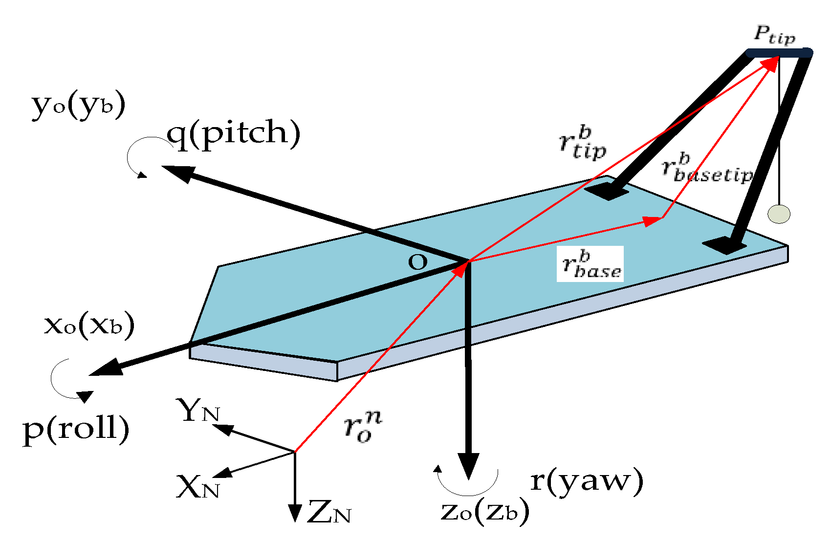
2.1. Motion Coordinate System

During the operation of the vessel on the sea surface, it is affected by the waves and generates six DOF of displacement: surge, sway, heave, roll, pitch, and yaw. To accurately describe the motion state of the system, reference coordinate systems are used in this paper: the North East Down (NED) frame (O–X_NY_NZ_N), the translation coordinate system frame (O–X_OY_OZ_O), and the Body-axis coordinate system (BODY) frame (O–X_bY_bZ_b); the positions of these coordinate systems are shown in Figure 2:

Equation (1) presents the mechanical equation of ship motion.

$$\left[\mathrm{M}+\mathrm{A}\left({\mathsf{\omega }}_1\right)\right]\ddot{x}+\mathrm{B}\left({\mathsf{\omega }}_1\right)\dot{x}+\mathrm{C}x=\mathrm{F}\left({\mathsf{\omega }}_1\right)$$

(1)

where x is the displacement vector of the vessel in all DOF (m); ω₁ is the oscillation frequency (Hz); M is the mass of the vessel (Kg); A(ω₁) is the additional quality (Kg); B(ω₁) is the damping ratio; C is the resilience factor; F(ω₁) is the harmonic excitation force (N).

Using Equation (1), the Amplitude Response Operator (RAO) can be employed to simulate the motion of the crane vessel under different sea conditions after wave disturbance [15].

It leads to:

$$\mathrm{RAO}\left({\mathsf{\omega }}_1\right)=\frac{x}{{\mathsf{\zeta }}_{\mathrm{a}}}=\frac{F_0}{\mathrm{C}-\left(\mathrm{M}+\mathrm{A}\left({\mathsf{\omega }}_1\right)\right){\mathsf{\omega }}_1{}^2+\mathrm{iB}\left({\mathsf{\omega }}_1\right){\mathsf{\omega }}_1}$$

(2)

where F₀ is the wave linear excitation force (N); ζ_a is the amplitude of the harmonic vector (m); using the MSS toolbox module in MATLAB, the response of the vessel in the different DOF can be modeled using the RAO principle.

In the coordinate system of Figure 2, the vector from the origin of the lifting vessel to the bottom of the crane is r^b_base; the vector from the bottom to the top lifting point of the crane is r^b_basetip.

The vector from the vessel’s origin to the lifting point of the crane can be obtained as:

$$r_{tip}^b=r_{base}^b+r_{basetip}^b$$

(3)

According to

Table 1. Vessel’s six DOF displacement.

6 DOF	Linear Velocity and Angular Velocity	Displacement and Offset Angle
surge	u	x
sway	v	y
heave	w	z
roll	p	ϕ
pitch	q	θ
yaw	r	Ψ

, the roll transformation matrix is:

$${\mathrm{R}}_{\mathrm{x},\mathsf{\varphi }}=\left[\begin{array}{ccc}1& 0& 0\\ 0& \cos \left(\mathsf{\varphi }\right)& -\sin \left(\mathsf{\varphi }\right)\\ 0& \sin \left(\mathsf{\varphi }\right)& \cos \left(\mathsf{\varphi }\right)\end{array}\right]$$

(4)

Similarly, the pitch and yaw transformation matrices can be drawn as:

$${\mathrm{R}}_{\mathrm{y},\mathsf{\theta }}=\left[\begin{array}{ccc}\cos \mathsf{\theta }& 0& \sin \mathsf{\theta }\\ 0& 1& 0\\ -\sin \left(\mathsf{\theta }\right)& 0& \cos \left(\mathsf{\theta }\right)\end{array}\right]$$

(5)

$${\mathrm{R}}_{\mathrm{y},\mathsf{\theta }}=\left[\begin{array}{ccc}\cos \mathsf{\theta }& 0& \sin \mathsf{\theta }\\ 0& 1& 0\\ -\sin \left(\mathsf{\theta }\right)& 0& \cos \left(\mathsf{\theta }\right)\end{array}\right]$$

(6)

The vessel’s rotation transformation matrix can be calculated as:

$$\begin{gathered} {\mathrm{R}}_{\mathrm{b}}^{\mathrm{n}}= \\ \left[\begin{array}{ccc}\cos \mathsf{\psi }\cos \mathsf{\theta }& -\sin \mathsf{\psi }\cos \mathsf{\varphi }+\cos \mathsf{\psi }\sin \mathsf{\theta }\sin \mathsf{\varphi }& \sin \mathsf{\psi }\sin \mathsf{\varphi }+\cos \mathsf{\psi }\cos \mathsf{\varphi }\sin \mathsf{\theta }\\ \sin \mathsf{\psi }\cos \mathsf{\theta }& \cos \mathsf{\psi }\cos \mathsf{\varphi }+\sin \mathsf{\varphi }\sin \mathsf{\theta }\sin \mathsf{\psi }& -\cos \mathsf{\psi }\sin \mathsf{\varphi }+\sin \mathsf{\theta }\sin \mathsf{\psi }\cos \mathsf{\varphi }\\ -\sin \mathsf{\theta }& \cos \mathsf{\theta }\sin \mathsf{\varphi }& \cos \mathsf{\theta }\cos \mathsf{\varphi }\end{array}\right] \end{gathered}$$

(7)

where ϕ is the angle of rotation of the x-axis; θ is the angle of rotation of the y-axis; ψ is the angle of rotation of the z-axis.

The coordinates of the lifting point can be expressed in the NED frame as:

$$P_{tip}^n=r_o^n+{\mathrm{R}}_{\mathrm{b}}^{\mathrm{n}}{r}_{tip}^b$$

(8)

When calculating the velocity in the NED frame, the fork product operator S is introduced to facilitate the calculation:

$$\mathrm{a}\times \mathrm{b}=S\left(a\right)\mathrm{b}$$

(9)

where S(a) is defined as:

$$S\left(a\right)=\left[\begin{array}{ccc}0& -a_3& a_2\\ a_3& 0& -a_1\\ -a_2& a_1& 0\end{array}\right]$$

(10)

$$a={\left[\begin{array}{ccc}{\mathrm{a}}_1& {\mathrm{a}}_2& {\mathrm{a}}_3\end{array}\right]}^{\mathrm{T}}$$

(11)

The velocity of the lifting point in the NED frame and the velocity of the crane vessel in the translation coordinate system are expressed as:

$${\dot{P}}_{tip}^{ n}=R_b^n{V}_{tip}^{ b}=R_b^n\left[V_o^b+{\mathsf{\omega }}_{nb}^{ b}\times r_{tip}^{ b}\right]=R_b^n\left[V_o^b+S({\mathsf{\omega }}_{nb}^{ b})r_{tip}^{ b}\right]$$

(12)

The rotation matrix relationship between the BODY frame and NED frame is:

$${\dot{R}}_b^n=R_b^n S\left({\mathsf{\omega }}_{nb}^b\right)$$

(13)

The acceleration of the lifting point is:

$$\begin{array}{l}{\ddot{P}}_{tip}^n=R_b^n\left[{\dot{V}}_o^b+S\left({\dot{\mathsf{\omega }}}_{nb}^b\right)r_{tip}^b+S\left({\mathsf{\omega }}_{nb}^b\right){\dot{r}}_{tip}^b+S\left({\mathsf{\omega }}_{nb}^b\right)V_o^b+S^2\left({\mathsf{\omega }}_{nb}^b\right)r_{tip}^b\right]\\ =R_b^n\left\{{\dot{V}}_o^b+\left[S\left({\dot{\mathsf{\omega }}}_{nb}^b\right)+S^2\left({\mathsf{\omega }}_{nb}^b\right)\right]r_{tip}^b+S\left({\mathsf{\omega }}_{nb}^b\right)\left[{\dot{r}}_{tip}^b+V_o^b\right]\right\}\end{array}$$

(14)

2.2. Wave Model

In this paper, the Guidance, Navigation and Control (GNC) module in the Marine Systems Simulator (MSS) MATLAB Simulink toolbox (version number 2020; Natick, MA, USA) is used. Waves are modelled using the JONSWAP wave energy spectrum. In order to simulate the effect of waves on the vessel, the wave elevation at any (x, y) position can be represented by superposition using the statistical principle.

$$\mathsf{\zeta }\left(\mathrm{x},\mathrm{y},\mathrm{t}\right)={\displaystyle \sum }_1^{\infty }{\mathsf{\zeta }}_{\mathrm{a}}\left(\mathrm{i}\right)\cos \left[\mathsf{\omega }\left(\mathrm{i}\right)\mathrm{t}+\mathsf{\phi }\left(\mathrm{i}\right)-\mathrm{k}\left(\mathrm{i}\right)\left(\mathrm{xcos}\left(\mathsf{\psi }\left(\mathrm{i}\right)\right)+\mathrm{ysin}\left(\mathsf{\psi }\left(\mathrm{i}\right)\right)\right)\right]$$

(15)

where ω(i) is the frequency of the harmonic vector (rad/s); φ(i) is the initial phase of the harmonic vector (rad); ψ(i) is the direction of the harmonic vector (rad); i is the number of the harmonic vector, t is the time (s). The relationship between the amplitude ζ_a (i) in equation (15) and wave frequency spectrum (S_ζ) is:

$${\mathsf{\zeta }}_{\mathrm{a}}=\sqrt{2{\mathrm{S}}_{\mathsf{\zeta }}\left({\mathsf{\omega }}_{\mathrm{i}}\right)\mathrm{d}\mathsf{\omega }}$$

(16)

In this paper, the JONSWAP wave energy spectrum is used to model and simulate the waves in level 4 sea state.

$$\mathrm{S}\left(\mathsf{\omega }\right)={\mathsf{\alpha }}_n\frac{{\mathrm{g}}^2}{{\mathsf{\omega }}^5}{e}^{[-\frac{5}{4}\left(\frac{{\mathsf{\omega }}_{\mathrm{p}}}{\mathsf{\omega }}{)}^4\right]}{\mathsf{\gamma }}^{\mathrm{e}[-\frac{1}{2}[\frac{\mathsf{\omega }-{\mathsf{\omega }}_{\mathrm{p}}}{{\mathsf{\sigma }\mathsf{\omega }}_{\mathrm{p}}}{)}^2]}$$

(17)

The spectral parameters of this spectrum are:

$$\mathsf{\sigma }=\left\{\begin{array}{c}0.07 \mathsf{\omega }⩽{\mathsf{\omega }}_{\mathrm{p}}\\ 0.09 \mathsf{\omega }⩾{\mathsf{\omega }}_{\mathrm{p}}\end{array}\right.$$

(18)

$$\mathsf{\alpha }=0.0076{\left(\frac{\mathrm{gx}}{{\mathrm{U}}^2}\right)}^{-0.22}$$

(19)

$${\mathsf{\omega }}_{\mathrm{p}}=22\left(\frac{\mathrm{g}}{\mathrm{U}}\right){\left(\frac{\mathrm{gx}}{{\mathrm{U}}^2}\right)}^{-0.33}$$

(20)

where α_n is a causeless constant; g is the acceleration of gravity (m/s²); U is the average wind speed (m/s); γ is the spectral peak factor and takes the value 3.3; ω_p is the spectral peak frequency (Hz).

2.3. Model of the Vessel Crane Load Motion System

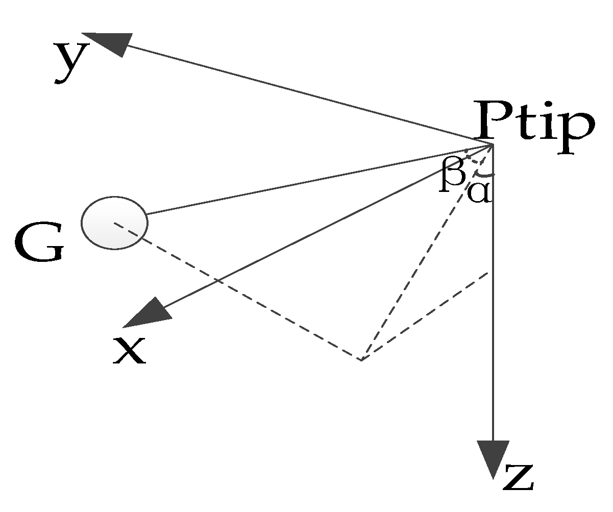
When the vessel crane is disturbed by waves, its motion is non-linear, and the system model is shown in Figure 3.

To be able to determine the position of the load, define its position in the NED system is Gⁿ, and G^p is the position of the load in the coordinate system with the lifting point (P_tip) as the original point; α, β is the inner angle of the plane and the outer angle of the plane. The vector relationship gives:

$$G^n=P_{tip}^n+G^P$$

(21)

G^p is expressed as:

$$\left\{\begin{array}{l}{\mathrm{x}}_{\mathrm{G}}\left(\mathrm{t}\right)=\left(\mathrm{L}+\mathrm{s}\left(\mathrm{t}\right)\right)\sin \mathsf{\alpha }\left(\mathrm{t}\right)\cos \mathsf{\beta }\left(\mathrm{t}\right)\\ {\mathrm{y}}_{\mathrm{G}}\left(\mathrm{t}\right)=-\left(\mathrm{L}+\mathrm{s}\left(\mathrm{t}\right)\right)\sin \mathsf{\beta }\left(\mathrm{t}\right)\\ {\mathrm{z}}_{\mathrm{G}}\left(\mathrm{t}\right)=\left(\mathrm{L}+\mathrm{s}\left(\mathrm{t}\right)\right)\cos \mathsf{\alpha }\left(\mathrm{t}\right)\cos \mathsf{\beta }\left(\mathrm{t}\right)\end{array}\right.$$

(22)

The total kinetic energy of the vessel crane system is:

$$\mathrm{T}=\frac{1}{2}{\mathrm{m}\dot{\mathrm{x}}}_{\mathrm{G}}^2\left(\mathrm{t}\right)+\frac{1}{2}{\mathrm{m}\dot{\mathrm{y}}}_{\mathrm{G}}^2\left(\mathrm{t}\right)+\frac{1}{2}{\mathrm{m}\dot{\mathrm{z}}}_{\mathrm{G}}^2\left(\mathrm{t}\right)$$

(23)

The total potential energy of the system is:

$$\mathrm{V}=\frac{1}{2}\mathrm{k}{\left(\mathrm{s}\left(\mathrm{t}\right)\right)}^2+\mathrm{mg}\left(\mathrm{L}+\mathsf{\lambda }\right)-\mathrm{mg}\left(\mathrm{L}+\mathrm{s}\left(\mathrm{t}\right)\right)\cos \mathsf{\alpha }\left(\mathrm{t}\right)\cos \mathsf{\beta }\left(\mathrm{t}\right)$$

(24)

The Lagrange function of the system is:

$$\mathrm{L}=\mathrm{T}-\mathrm{V}$$

(25)

According to the Lagrange equation:

$$\frac{\mathrm{d}}{\mathrm{dt}}\left(\frac{\partial {\mathrm{L}}_{\mathrm{a}}}{\partial { \dot{\mathrm{q}}}_{\mathrm{j}}}\right)-\frac{\partial {\mathrm{L}}_{\mathrm{a}}}{\partial {\mathrm{q}}_{\mathrm{j}}}=0$$

(26)

The second order differential equation for the dynamics of the vessel crane system is derived by simplification:

$$\begin{array}{cc}\hfill \ddot{\mathrm{s}}\left(\mathrm{t}\right)& =\left(\mathrm{L}+\mathrm{s}\left(\mathrm{t}\right)\right){\dot{\mathsf{\alpha }}}^2\left(\mathrm{t}\right){\cos }^2\mathsf{\beta }\left(\mathrm{t}\right)-\frac{\mathrm{k}}{\mathrm{m}}\mathrm{s}\left(\mathrm{t}\right)\hfill \\ & +\left(\mathrm{L}+\mathrm{s}\left(\mathrm{t}\right)\right){\dot{\mathsf{\beta }}}^2\left(\mathrm{t}\right)+\mathrm{gcos}\mathsf{\alpha }\left(\mathrm{t}\right)\cos \mathsf{\beta }\left(\mathrm{t}\right)\hfill \end{array}$$

(27)

$$\ddot{\mathsf{\alpha }}\left(\mathrm{t}\right)=-\frac{2 \dot{\mathrm{s}}\left(\mathrm{t}\right) \dot{\mathsf{\alpha }}\left(\mathrm{t}\right)}{\mathrm{L}+\mathrm{s}\left(\mathrm{t}\right)}+2 \dot{\mathsf{\alpha }}\left(\mathrm{t}\right) \dot{\mathsf{\beta }}\left(\mathrm{t}\right)\frac{\sin \mathsf{\beta }\left(\mathrm{t}\right)}{\cos \mathsf{\beta }\left(\mathrm{t}\right)}-\frac{\mathrm{gsin}\mathsf{\alpha }\left(\mathrm{t}\right)}{\left(\mathrm{L}+\mathrm{s}\left(\mathrm{t}\right)\right)\cos \mathsf{\beta }\left(\mathrm{t}\right)}$$

(28)

$$\begin{array}{cc}\hfill \ddot{\mathsf{\beta }}\left(\mathrm{t}\right)& =-\frac{2 \dot{\mathrm{s}}\left(\mathrm{t}\right) \dot{\mathsf{\beta }}\left(\mathrm{t}\right)}{\mathrm{L}+\mathrm{s}\left(\mathrm{t}\right)}-{ \dot{\mathsf{\alpha }}}^2\left(\mathrm{t}\right)\sin \mathsf{\beta }\left(\mathrm{t}\right)\cos \mathsf{\beta }\left(\mathrm{t}\right)\hfill \\ & -\frac{\mathrm{g}}{\left(\mathrm{L}+\mathrm{s}\left(\mathrm{t}\right)\right)}\cos \mathsf{\alpha }\left(\mathrm{t}\right)\sin \mathsf{\beta }\left(\mathrm{t}\right)\hfill \end{array}$$

(29)

where L is the length of the rope at rest (m); λ is the extension of the rope at rest (m); s is the rope elongation in motion (m); m is the mass of the load (kg).

2.4. Hydrodynamic Calculations of Splash Zones

During offshore operations, the load is subject to hydrodynamic force that may break the rope when it passes through the splash zone. The equation of motion can be derived from the force applied to the load as follows:

$$\mathrm{mg}={\mathrm{F}}_{\mathrm{t}}+{\mathrm{F}}_{\mathrm{h}}$$

(30)

where F_t is the elasticity of the rope (N); F_h is the hydrodynamic force on the rope (N).

From the differential equation for the second-order dynamics of the rope crane, the elongation of the rope can be determined as s. The elasticity of the rope can therefore be expressed as:

$${\mathrm{F}}_{\mathrm{t}}=\mathrm{m}\ddot{\mathrm{s}}+\mathrm{z} \dot{\mathrm{s}}+\mathrm{ks}$$

(31)

where z is the damping factor (N·s/m); k is the elasticity factor (N/m).

Since the modelling of waves has been done in the previous section, the hydrodynamic forces can be obtained here:

$${\mathrm{F}}_{\mathrm{h}}={\mathrm{F}}_{\mathrm{B}}+{\mathrm{F}}_{\mathrm{A}}+{\mathrm{F}}_{\mathrm{D}}$$

(32)

where F_B, F_A, and F_D are the forces caused by buoyancy, added mass, and drag effects, respectively (N). In this paper it is assumed that the load is a sphere with a diameter of d = 2 m. The hydrodynamic force can therefore be simplified as [16]:

When d_p > 0:

$${\mathrm{F}}_{\mathrm{h}}={\mathrm{m}}_{\mathrm{a}}\left(\ddot{\mathrm{z}}-{\ddot{\mathrm{z}}}_0\right)\left(\frac{{\mathrm{d}}_{\mathrm{p}}}{\mathrm{d}}\right)+\frac{1}{2}{\mathsf{\rho }\mathrm{C}}_{\mathrm{D}}{\mathrm{A}}_{\mathrm{p}}\left( \dot{\mathrm{z}}-{ \dot{\mathrm{z}}}_0\right)\left| \dot{\mathrm{z}}-{ \dot{\mathrm{z}}}_0\right|\left(\frac{{\mathrm{d}}_{\mathrm{p}}}{\mathrm{d}}\right)+{\mathsf{\rho }\mathrm{gV}}_{\mathrm{p}}\left({\mathrm{d}}_{\mathrm{p}}\right)$$

(33)

When d_p ≤ 0:

$${\mathrm{F}}_{\mathrm{h}}=0$$

(34)

where d_p is the distance below the surface of the sea (m); m_a is the additional mass of the spherical load (kg); V_p(d_p) is the volume of the object submerged in water (m³); d is the diameter of the object to be lifted (m); ρ is the density of seawater, ρ ≈ 1024 (kg/m³). d_p can be found from the distance between the load and the water surface (z_w):

$${\mathrm{d}}_{\mathrm{p}}=\left\{\begin{array}{c}-{\mathrm{z}}_{\mathrm{w}}, -d\le {\mathrm{z}}_{\mathrm{w}}\le 0\\ d , {\mathrm{z}}_{\mathrm{w}}\le -d\\ 0 , {\mathrm{z}}_{\mathrm{w}}\ge 0\end{array}\right.$$

(35)

When z_w = 0, the load just touches the water surface. The remaining terms in Equation (33) can be derived from the following equation:

$${\mathrm{m}}_{\mathrm{a}}=\frac{1}{2}\mathsf{\rho }\left(\frac{4}{3}\mathsf{\pi }{\left(\frac{\mathrm{d}}{2}\right)}^2\right)$$

(36)

$${\mathrm{V}}_{\mathrm{p}}\left({\mathrm{d}}_{\mathrm{p}}\right)=\frac{\mathsf{\pi }}{3}{\mathrm{d}}_{\mathrm{p}}^2\left(\frac{3}{2}\mathrm{d}-{\mathrm{d}}_{\mathrm{p}}\right)$$

(37)

$${\mathrm{A}}_{\mathrm{p}}=\mathsf{\pi }{\left(\frac{\mathrm{d}}{2}\right)}^2$$

(38)

2.5. Prediction of Heave Displacement Data

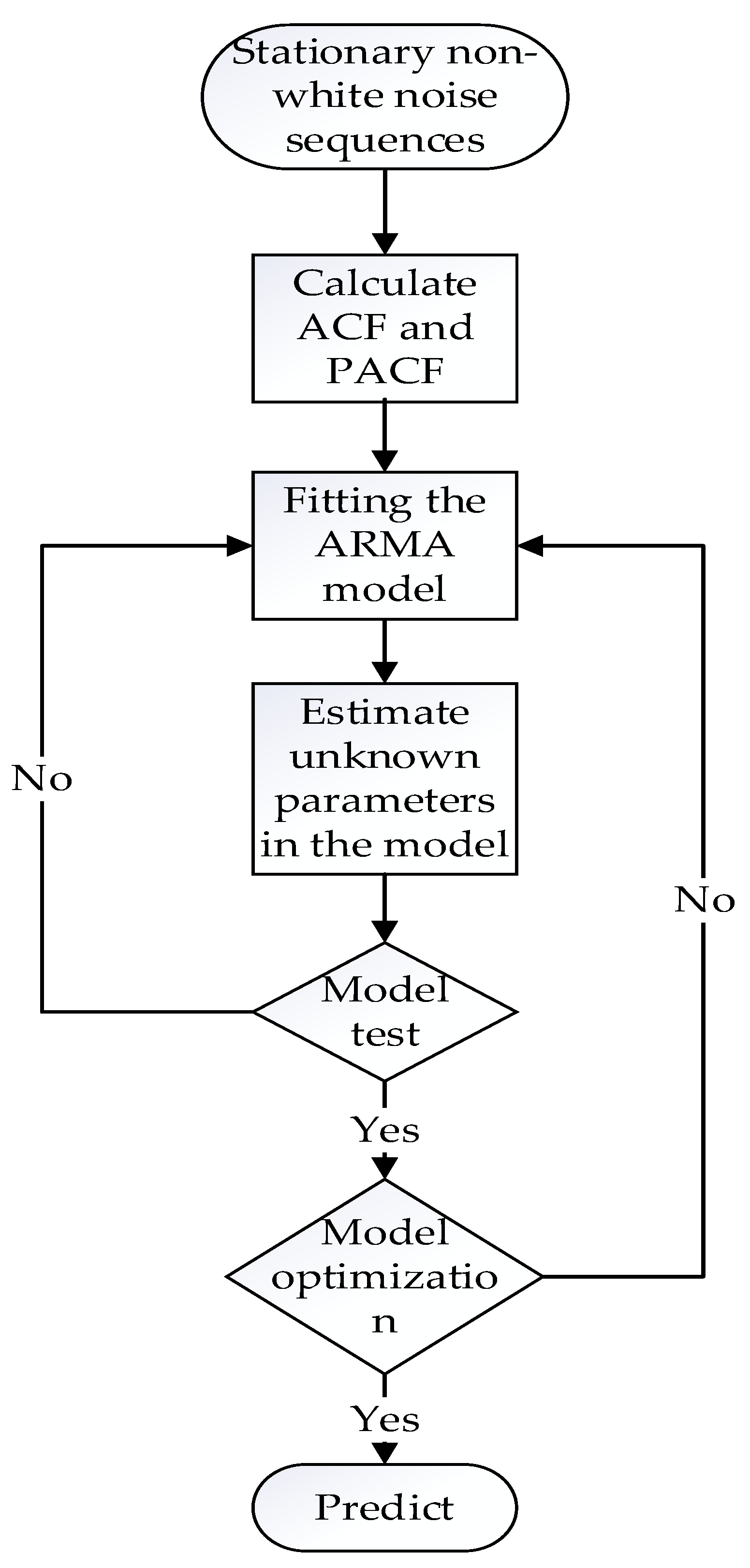
The detection and mechanical links usually cause time lags in the system, which seriously affects the compensation accuracy and stability. In order to reduce this effect, forecast of heave motion is often used to ensure the safety and efficiency of operations in advance [17]. Prediction variance increases with the number of periods. This paper uses time series prediction algorithm with the principle of minimum forecast variance. The collected time series are fitted with the autoregressive moving average (ARMA) model [18]. ARMA effectively uses a small amount of historical data to rapidly track the current degradation trend. And the least squares method is used for parameter estimation after fitting the ARMA model. The least square estimation is the smallest estimation of a residual sum. Model testing is to check whether the residual sequence has incomplete information. Then, as Figure 4 shows, it will predict the next sampling moment of heave displacement data.

The time series prediction algorithm is only applicable to smooth and non-white noise series. Therefore, the smoothness test must be performed before the time series can be predicted. When the time series is inherently non-smooth, it can be predicted when it is smooth after differencing. It is needed that the order of difference is not too large, otherwise the prediction accuracy will be low.

The expression for ARMA (p, q) is:

$${\mathrm{x}}_{\mathrm{t}}={\mathsf{\varphi }}_0+{\mathsf{\varphi }}_1{\mathrm{x}}_{\mathrm{t}-1}+\cdots +{\mathsf{\varphi }}_{\mathrm{p}}{\mathrm{x}}_{\mathrm{t}-\mathrm{p}}+{\mathsf{\epsilon }}_{\mathrm{t}}-{\mathsf{\theta }}_1{\mathsf{\epsilon }}_{\mathrm{t}-1}-\cdots -{\mathsf{\theta }}_{\mathrm{q}}{\mathsf{\epsilon }}_{\mathrm{t}-\mathrm{q}}$$

(39)

where ϕ₁, ϕ₂, …, ϕ_p denote the autoregressive coefficient, θ₁, θ₂, …, θ_q denote the sliding average coefficient, ε_t denotes the white noise sequence. The expected value of the ε_t is 0 and the variance value of the ε_t is σ_ε. The following are statistical characteristics:

Average value:

$$\mathrm{E}\left({\mathrm{x}}_{\mathrm{t}}\right)=\frac{{\mathsf{\Phi }}_0}{1-{\mathsf{\Phi }}_1-\cdots -{\mathsf{\Phi }}_{\mathrm{p}}}$$

(40)

Variance:

$$\mathrm{Var}\left({\mathrm{x}}_{\mathrm{t}}\right)={\displaystyle \sum }_{\mathrm{j}=0}^{\infty }{\mathrm{G}}_{\mathrm{j}}{}^2{\mathsf{\sigma }}_{\mathsf{\epsilon }}{}^2$$

(41)

Autocovariance:

$$\mathsf{\gamma }\left(\mathrm{k}\right)={\mathsf{\sigma }}_{ϵ}{}^2{\displaystyle \sum }_{\mathrm{i}=0}^{\infty }{\mathrm{G}}_{\mathrm{j}}{\mathrm{G}}_{\mathrm{j}+\mathrm{k}}$$

(42)

Autocorrelation coefficient:

$$\mathsf{\rho }\left(\mathrm{k}\right)=\frac{\mathsf{\gamma }\left(\mathrm{k}\right)}{\mathsf{\gamma }\left(0\right)}=\frac{{\displaystyle {\displaystyle \sum }_{\mathrm{j}=0}^{\infty }}{\mathrm{G}}_{\mathrm{j}}{\mathrm{G}}_{\mathrm{j}+\mathrm{k}}}{{\displaystyle {\displaystyle \sum }_{\mathrm{j}=0}^{\infty }}{\mathrm{G}}_{\mathrm{j}}{}^2}$$

(43)

$$\left\{\begin{array}{l}{\mathrm{G}}_0=1\\ {\mathrm{G}}_{\mathrm{k}}={\displaystyle {\displaystyle \sum }_{\mathrm{j}=1}^{\mathrm{k}}}{\mathsf{\Phi }}_{\mathrm{j}}{}^{\prime }{\mathrm{G}}_{\mathrm{k}-\mathrm{j}}-{\mathsf{\theta }}_{\mathrm{k}}{}^{\prime },\mathrm{k}⩾1\end{array}\right.{\mathsf{\Phi }}_{\mathrm{j}}{}^{\prime }=\left\{\begin{array}{c}{\mathsf{\Phi }}_{\mathrm{j}},1⩽\mathrm{j}⩽\mathrm{p}\\ 0,\mathrm{j}>\mathrm{p}\end{array}\right.{\mathsf{\theta }}_{\mathrm{k}}{}^{\prime }=\left\{\begin{array}{c}{\mathsf{\theta }}_{\mathrm{k}},1⩽\mathrm{k}⩽\mathrm{q}\\ 0,\mathrm{k}>\mathrm{q}\end{array}\right.$$

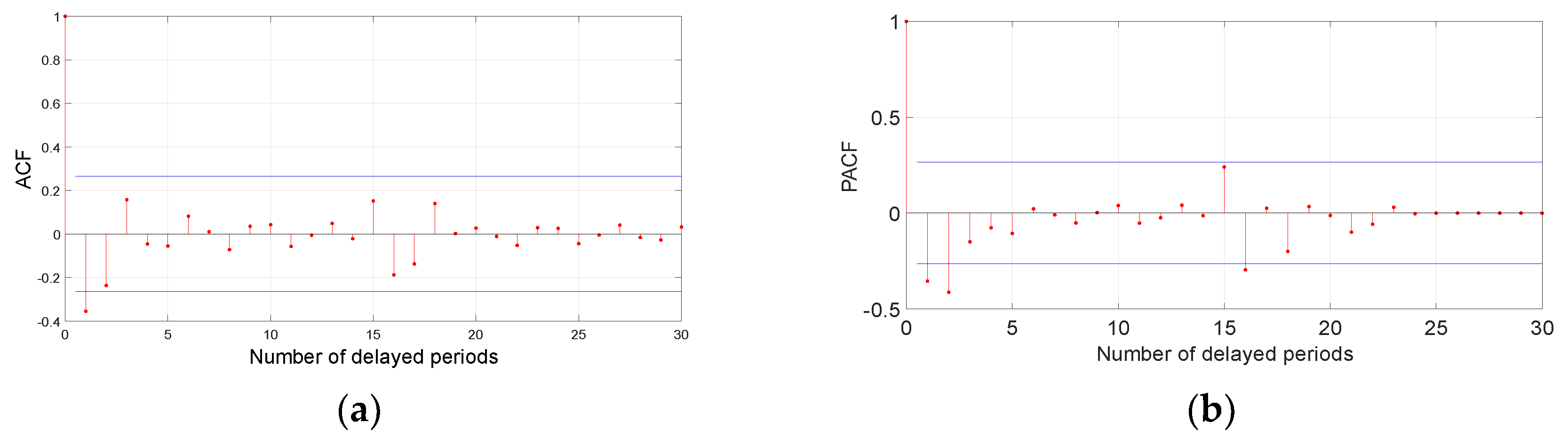
According to

Table 2. Trailing and truncation characteristics of time series models.

Model	ACF	PACF
AR(p)	trailing	p-order truncation
MA(q)	q-order truncation	trailing
ARMA(p,q)	trailing	trailing

, the autocorrelation coefficient (ACF) and partial autocorrelation coefficient (PACF) of the sample are used to identify the model. It can determine the order of undetermined model parameters p and q. After passing the time series smoothness test, the smooth non-white noise series will be predicted according to the Figure 4:

The heave displacement autocorrelation test chart and autocorrelation test chart are shown in Figure 5a,b:

2.6. Mathematical Model of PMSM

PMSM has the advantages of reliable operation, high efficiency, and a small size. So, this paper uses PMSM as the compensation mechanism. As shown in Figure 1, it can make the rope extend and contract.

The stator voltage equation is:

$$\left\{\begin{array}{c}{\mathrm{u}}_{\mathrm{d}}=\frac{{\mathrm{d}\mathsf{\psi }}_{\mathrm{d}}}{\mathrm{dt}}+{\mathrm{R}}_{\mathrm{s}}{\mathrm{i}}_{\mathrm{d}}-{\mathsf{\psi }}_{\mathrm{q}}\mathsf{\omega }\\ {\mathrm{u}}_{\mathrm{q}}=\frac{{\mathrm{d}\mathsf{\psi }}_{\mathrm{q}}}{\mathrm{dt}}+{\mathrm{R}}_{\mathrm{s}}{\mathrm{i}}_{\mathrm{q}}+{\mathsf{\psi }}_{\mathrm{d}}\mathsf{\omega }\end{array}\right.$$

(44)

The equation for the flux linkage component is:

$$\left\{\begin{array}{l}{\mathsf{\psi }}_{\mathrm{d}}={\mathrm{L}}_{\mathrm{d}}{\mathrm{i}}_{\mathrm{d}}+{\mathsf{\psi }}_{\mathrm{f}} \\ {\mathsf{\psi }}_{\mathrm{q}}={\mathrm{L}}_{\mathrm{q}}{\mathrm{i}}_{\mathrm{q}} \end{array}\right.$$

(45)

The electromagnetic torque equation is:

$$\begin{array}{cc}\hfill {\mathrm{T}}_{\mathrm{e}}& =\frac{3}{2}{\mathrm{P}}_{\mathrm{n}}\left({\mathsf{\psi }}_{\mathrm{d}}{\mathrm{i}}_{\mathrm{q}}-{\mathsf{\psi }}_{\mathrm{q}}{\mathrm{i}}_{\mathrm{d}}\right)\hfill \\ & =\frac{3}{2}{\mathrm{P}}_{\mathrm{n}}\left[{\mathsf{\psi }}_{\mathrm{f}}{\mathrm{i}}_{\mathrm{q}}+\left({\mathrm{L}}_{\mathrm{d}}-{\mathrm{L}}_{\mathrm{q}}\right){\mathrm{i}}_{\mathrm{d}}{\mathrm{i}}_{\mathrm{q}}\right]\hfill \end{array}$$

(46)

The equation of motion is:

$${\mathrm{T}}_{\mathrm{e}}-{\mathrm{T}}_{\mathrm{L}}={\mathrm{J}}_{\mathrm{m}}\frac{{\mathrm{d}\mathsf{\omega }}_{\mathrm{r}}}{\mathrm{dt}}+{\mathrm{B}\mathsf{\omega }}_{\mathrm{r}}$$

(47)

where ω_r is the mechanical angular velocity of the motor (rad/s); ω is the electrical angular of the motor (rad/s); u_d, u_q; ψ_d,ψ_q; i_d, i_q; L_d, L_q are the respectively the voltages (V), flux linkage component (Wb), current (A) and inductance (H) components expressed in the d-q frame; R_s is the stator equivalent resistance (Ω); ψ_f is the permanent magnet flux of the rotor (Wb); T_L is the load torque (N·m); J_m is the moment of inertia (kg/m²); T_e is the electromagnetic torque (N·m); P_n is the number of pole pairs.

In this paper, the reluctance torque is ignored because the surface-mounted PMSM is considered (L_d = L_q = L). So, the corresponding electromagnetic torque equation can be simplified as:

$${\mathrm{T}}_{\mathrm{e}}=\frac{3}{2}{\mathrm{P}}_{\mathrm{n}}{\mathsf{\psi }}_{\mathrm{f}}{\mathrm{i}}_{\mathrm{q}}$$

(48)

Combining Equations (44), (46), and (47), the state equation for the motor in the d-q coordinate system can be obtained as:

$$\frac{\mathrm{d}}{\mathrm{dt}}\left[\begin{array}{c}{\mathrm{i}}_{\mathrm{d}}\\ {\mathrm{i}}_{\mathrm{q}}\\ {\mathsf{\omega }}_{\mathrm{r}}\end{array}\right]=\left[\begin{array}{ccc}-\frac{{\mathrm{R}}_{\mathrm{s}}}{\mathrm{L}}& {\mathrm{P}}_{\mathrm{n}}{\mathsf{\omega }}_{\mathrm{r}}& 0\\ -{\mathrm{P}}_{\mathrm{n}}{\mathsf{\omega }}_{\mathrm{r}}& -\frac{\mathrm{R}}{\mathrm{L}}& -\frac{{\mathrm{P}}_{\mathrm{n}}{\mathsf{\psi }}_{\mathrm{f}}}{\mathrm{L}}\\ 0& \frac{1.5{\mathrm{P}}_{\mathrm{n}}{\mathsf{\psi }}_{\mathrm{f}}}{{\mathrm{J}}_{\mathrm{m}}}& -\frac{\mathrm{B}}{{\mathrm{J}}_{\mathrm{m}}}\end{array}\right]\left[\begin{array}{c}{\mathrm{i}}_{\mathrm{d}}\\ {\mathrm{i}}_{\mathrm{q}}\\ {\mathsf{\omega }}_{\mathrm{r}}\end{array}\right]+\left[\begin{array}{c}\frac{{\mathrm{u}}_{\mathrm{d}}}{\mathrm{L}}\\ \frac{{\mathrm{u}}_{\mathrm{q}}}{\mathrm{L}}\\ -\frac{{\mathrm{T}}_{\mathrm{L}}}{{\mathrm{J}}_{\mathrm{m}}}\end{array}\right]$$

(49)

In this paper, a maximum Torque per Ampere strategy is used for motor control. So, i_d is controlled to be 0 and i_q current is used for torque control in current loop which will be described in the next section.

3. Fractional-Order PID Controller

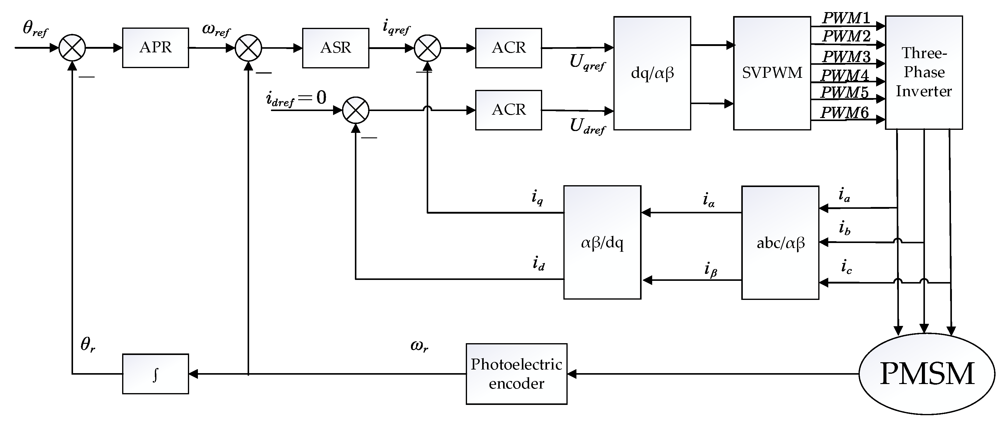
PMSM control used in this paper is based on a triple closed-loop control structure. The three-loop control diagram is shown in Figure 6.

Closed-loop control of the system can improve the following performance of the motor [19]. A triple closed-loop structure usually uses the PID controllers. However, it has poor tracking performance due to the complex wave disturbance of the system. Because differential and integral operators can only be 0 or 1 orders for P, PI, PD, or PID controllers, the number of DOF in terms of controller parameters is small. This paper uses fractional-order PID controllers instead of traditional PID controllers in the automatic position regulator (APR) [20]. Automatic speed regulator (ASR) and automatic current regulator (ACR) still use PID controller. In order to avoid the uncertainty and complexity of manual tuning of a fractional-order PID controller, the next section applies artificial intelligence based algorithms. It can refine their parameters and improve the accuracy of the control. For the speed loop where a PID controller is used, there are also problems with complex models and speed overshoot [21].

3.1. Basic Principle of FOPID Controller

During wave compensation, it is necessary to accurately place the load at the set position. Therefore, the position loop is particularly important in the three loops control. Because there is an integral link in the position loop, and the integral link will lead to the delay of the system. Although a given position signal can reach the desired position, the speed command will still maintain a high value due to the delay effect. The motor will continue to rotate at a high speed, and it will be forced to stop due to reverse rotation due to position overshoot. So, APR is set as the proportional controller.

If the servo system wants to satisfy that the position loop has no overshoot, the proportional gain of the system cannot be too large. This cannot meet the rapid response requirements of the system. The response speed and small steady-state error of the system limits the proportional gain of the controller. As a result, the rapidity and high accuracy of the control system cannot be guaranteed.

The concept of fractional-order calculus was developed in the seventeenth century [22]. Fractional-order calculus extends the traditional integral and differential operators from the integer order to the real order. It offers a greater range of feasibility and flexibility in system modelling and controller design methods than the classical integer order approach. It also provides a better closed-loop response and greater robustness to uncertainty [23]. Open-loop frequency response experiments are performed on the PMSM. It shows that in the middle and high-frequency range, the frequency response of the fractional-order model is closer to the actual frequency response of PMSM than the integer-order model [24]. FOPID controller can suppress the high-frequency and low-frequency disturbances. In other words, the robustness of the fractional-order controller is much better than the traditional PID controller. The transfer function of FOPID is shown in Equation (50):

$${\mathrm{G}}_{\mathrm{c}}\left(\mathrm{s}\right)={\mathrm{K}}_{\mathrm{p}}+\frac{{\mathrm{K}}_{\mathrm{i}}}{{\mathrm{s}}^{\mathsf{\lambda }}}+{\mathrm{K}}_{\mathrm{d}}{\mathrm{s}}^{\mathsf{\mu }}$$

(50)

When the values of [λ, μ] are taken as [0, 0], [1, 0], [0, 1], [1, 1]. Fractional-order PID controller can be considered as a classical P, PI, PD, and PID controller. In this paper, 1/s^λ can be approached by connecting an integer-order integrator and a fractional-order differentiator approximated by an Oustaloup filter. As shown in Figure 7, and Equation (50) 5 parameters have to be determined to tune a FOPID. If the five parameters of the controller are set appropriately, a better control than conventional PID controllers can be achieved [25].

In order to ensure stability of the control loop, the open-loop frequency characteristics of the system need to satisfy the following two conditions:

$$\mathrm{Arg}\left[\mathrm{G}\left({\mathrm{j}\mathsf{\omega }}_{\mathrm{c}}\right)\right]=-\mathsf{\pi }+{\mathsf{\psi }}_{\mathrm{m}}$$

(51)

$$\left|\mathrm{G}\left({\mathrm{j}\mathsf{\omega }}_{\mathrm{c}}\right)\right|=1$$

(52)

where ψ_m is the phase margin (rad), ω_c is the gain crossover frequency (rad/s).

If the control loop needs to be strongly robust, it needs to satisfy:

$${\left(\frac{\mathrm{d}\left(\mathrm{Arg}\left[\mathrm{G}\left(\mathrm{j}\mathsf{\omega }\right)\right]\right)}{\mathrm{d}\mathsf{\omega }}\right)}_{\mathsf{\omega }={\mathsf{\omega }}_{\mathrm{c}}}=0$$

(53)

The constraint equation can be derived as:

$$\begin{array}{l}\arctan \frac{{\mathrm{K}}_{\mathrm{d}}{\mathsf{\omega }}_{\mathrm{c}}{}^{\mathsf{\mu }}\sin \left(\frac{\mathsf{\pi }\mathsf{\mu }}{2}\right)-{\mathrm{K}}_{\mathrm{i}}{\mathsf{\omega }}_{\mathrm{c}}{}^{-\mathsf{\lambda }}\sin \left(\frac{\mathsf{\pi }\mathsf{\lambda }}{2}\right)}{{\mathrm{K}}_{\mathrm{p}}+{\mathrm{K}}_{\mathrm{i}}{\mathsf{\omega }}_{\mathrm{c}}{}^{-\mathsf{\lambda }}\cos \left(\frac{\mathsf{\pi }\mathsf{\lambda }}{2}\right)+{\mathrm{K}}_{\mathrm{d}}{\mathsf{\omega }}_{\mathrm{c}}{}^{\mathsf{\mu }}\cos \left(\frac{\mathsf{\pi }\mathsf{\mu }}{2}\right)}-\arctan \left({\mathsf{\omega }}_{\mathrm{c}}\mathrm{T}\right)\\ =-\mathsf{\pi }+{\mathsf{\psi }}_{\mathrm{m}}\end{array}$$

(54)

$$\begin{array}{l}\frac{\sqrt{{\left({\mathrm{K}}_{\mathrm{p}}+{\mathrm{K}}_{\mathrm{i}}{\mathsf{\omega }}_{\mathrm{c}}{}^{-\mathsf{\lambda }}\cos \left(\frac{\mathsf{\pi }\mathsf{\lambda }}{2}\right)+{\mathrm{K}}_{\mathrm{d}}{\mathsf{\omega }}_{\mathrm{c}}{}^{\mathsf{\mu }}\cos \left(\frac{\mathsf{\pi }\mathsf{\mu }}{2}\right)\right)}^2+{\left({\mathrm{K}}_{\mathrm{d}}{\mathsf{\omega }}_{\mathrm{c}}{}^{\mathsf{\mu }}\sin \left(\frac{\mathsf{\pi }\mathsf{\mu }}{2}\right)-{\mathrm{K}}_{\mathrm{i}}{\mathsf{\omega }}_{\mathrm{c}}{}^{-\mathsf{\lambda }}\sin \left(\frac{\mathsf{\pi }\mathsf{\lambda }}{2}\right)\right)}^2}}{\sqrt{1+{\left({\mathrm{T}\mathsf{\omega }}_{\mathrm{c}}\right)}^2}}\\ =1\end{array}$$

(55)

$$\frac{{\mathrm{A}}^{\prime }\mathrm{B}-\mathrm{A}{\mathrm{B}}^{\prime }}{{\mathrm{A}}^2+{\mathrm{B}}^2}-\frac{\mathrm{T}}{1+{\left({\mathrm{T}\mathsf{\omega }}_{\mathrm{c}}\right)}^2}=0$$

(56)

$$\mathrm{A}={\mathrm{K}}_{\mathrm{d}}{\mathsf{\omega }}^{\mathsf{\mu }}\sin \left(\frac{\mathsf{\pi }\mathsf{\mu }}{2}\right)-{\mathrm{K}}_{\mathrm{i}}{\mathsf{\omega }}^{-\mathsf{\lambda }}\sin \left(\frac{\mathsf{\pi }\mathsf{\lambda }}{2}\right)$$

(57)

$$\mathrm{B}={\mathrm{K}}_{\mathrm{p}}+{\mathrm{K}}_{\mathrm{i}}{\mathsf{\omega }}^{-\mathsf{\lambda }}\cos \left(\frac{\mathsf{\pi }\mathsf{\lambda }}{2}\right)+{\mathrm{K}}_{\mathrm{d}}{\mathsf{\omega }}^{\mathsf{\mu }}\cos \left(\frac{\mathsf{\pi }\mathsf{\mu }}{2}\right)$$

(58)

$${\mathrm{A}}^{\prime }={\mathsf{\mu }\mathrm{K}}_{\mathrm{d}}{\mathsf{\omega }}^{\mathsf{\mu }-1}\sin \left(\frac{\mathsf{\pi }\mathsf{\mu }}{2}\right)+{\mathsf{\lambda }\mathrm{K}}_{\mathrm{i}}{\mathsf{\omega }}^{-\mathsf{\lambda }-1}\sin \left(\frac{\mathsf{\pi }\mathsf{\lambda }}{2}\right)$$

(59)

$${\mathrm{B}}^{\prime }=-{\mathsf{\lambda }\mathrm{K}}_{\mathrm{i}}{\mathsf{\omega }}^{-\mathsf{\lambda }-1}\cos \left(\frac{\mathsf{\pi }\mathsf{\lambda }}{2}\right)+{\mathsf{\mu }\mathrm{K}}_{\mathrm{d}}{\mathsf{\omega }}^{\mathsf{\mu }-1}\cos \left(\frac{\mathsf{\pi }\mathsf{\mu }}{2}\right)$$

(60)

where T is the time constant of the controlled system. In the presented study, the phase margin of the controller is chosen to be 45° and the gain crossover frequency is chosen to be 80 rad/s.

3.2. Improved FOPID Based on GAPSO Algorithm

The position loop of PMSM allows accurate positioning. It is also an essential part of the entire triple closed-loop control system for stable and highly accurate operation. The objective of this paper is to propose control solutions in order to improve the tracking of the reference position for the load. Optimization of the values of the five parameters of the controller can increase the performance of the control system and achieve robustness. The calculation process of FOPID is complicated and it is necessary to select appropriate crossover frequency and phase margin. It is obvious that the tuning of the parameters of the FOPID will affect the controller performance. They can improve the robustness and performance of system. However, this will certainly make the parameter adjustment process more complicated [26]. So, these parameters should be chosen carefully. To be able to determine relevant parameters for the FOPID, an optimization algorithm based on a combination of genetic algorithm and particle swarm algorithm (GAPSO algorithm) is used to optimize the parameters.

Both genetic algorithms and particle swarm algorithms are optimization algorithms based on population search. Their flowchart is shown in Figure 8. More details about these two algorithms can be found in reference [27,28] for interested readers. However, particle swarm algorithm can easily lead to local optimum solutions, while genetic algorithms are slower to find the optimum. This paper introduces an optimization algorithm that includes a genetic algorithm into the particle swarm algorithm. This GAPSO algorithm is based on double population. The particles with better fitness obtained by PSO algorithm will start crossover and variation. Because GA has no selection link, the running time of the GAPSO program is faster than GA. Its flowchart is shown in Figure 9. Particle swarm algorithms can improve the convergence speed of the overall algorithm, while genetic algorithms can expand the search space and improve the limitations of particle swarm algorithms. The use of the GAPSO algorithm to adjust fractional-order PID controller parameters expands the solution space, while avoiding the problems of complex operations.

The first population mentioned above serves mainly as detection, which has a higher probability of crossover and variation. It can generate completely new individuals for the population and enhance global search capabilities. The second population is called the development population and it has fast convergence as its main goal. It has a relatively low probability of crossover and variation, which is suitable for local searches for well-adapted individuals. At the end of a cycle of the algorithm, the individuals with the highest fitness of the other population are introduced into their own population. It enhances interactions between populations and speeds up the search, while preventing incomplete solutions from being obtained. A more complete description of the GAPSO algorithm can be found in [29].

The parameters of the fractional-order PID controller are adjusted by GAPSO algorithm. Both populations are 100 in number and 5 iterations are performed. The range of P,I,D and μ,λ are set as [0.01, 300] and [0.01, 2]. After the parameters are introduced into the system, the fitness is determined based on the ITAE in (62). Finally, after algorithm iteration and calculation, the parameters of fractional-order controller are:

$${\mathrm{G}}_{\mathrm{GAPSO}}\left(\mathrm{s}\right)=281.977+\frac{209.12}{{\mathrm{s}}^{0.174}}+267.41{\mathrm{s}}^{0.16}$$

(61)

4. Presentation and Discussion of Test Results

In this paper, the effect of compensation is analyzed using a MATLAB/Simulink to represent the overall system for crane operation in a level 4 sea state. The sea level is Z = 0 m and the crane point height (P_tip in Figure 2) is Z = −25 m. The simulation parameters are shown in

Table 3. Simulation parameters of system.

Parameters	Value	Parameters	Value
Vessel draft	6 m	Load diameter	2 m
Vessel width	19.2 m	Wave spreading factor	1
Vessel quality	63,622 kg	Significant wave height	3 m
Elasticity of the rope	8.2 × 106 N/m	Mean wave direction	Pi/4 rad
Load mass	21,000 kg	The density of water	1025 kg/m3

.

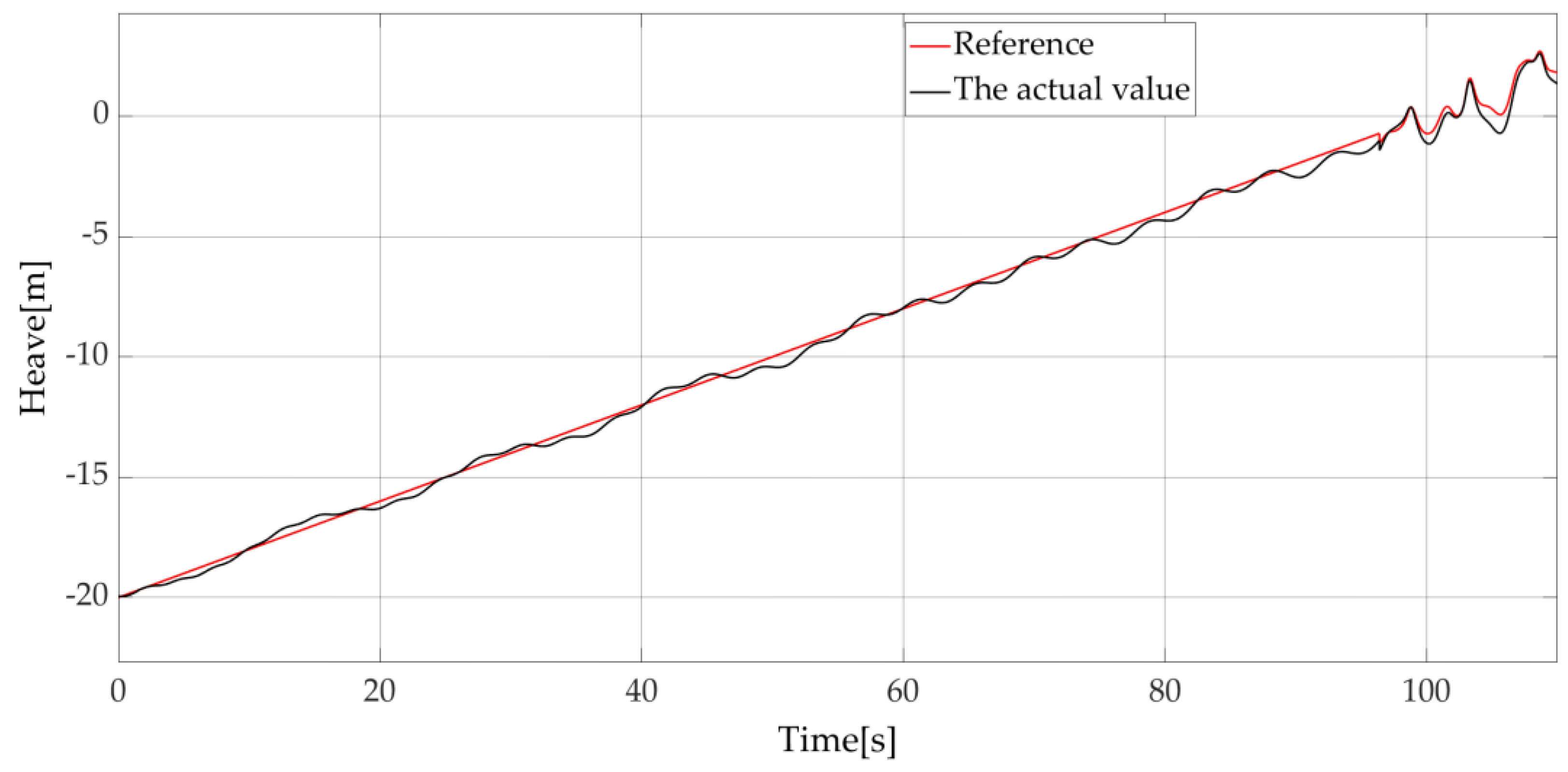
The vessel is influenced by the waves to move up and down in the direction of the heave. After the crane load enters the water and is influenced by the hydrodynamic force, the line of the reference position will become curves. Due to wave effects, the tracking of the position of the crane load to the reference position is subject to strong errors. To illustrate the wave influence, a first simulation is done with a rope length equal to L = 5 m, and a load descending speed equal to V = 0.2 m/s. The position and heave error of the load in this case without compensation are shown in Figure 10.

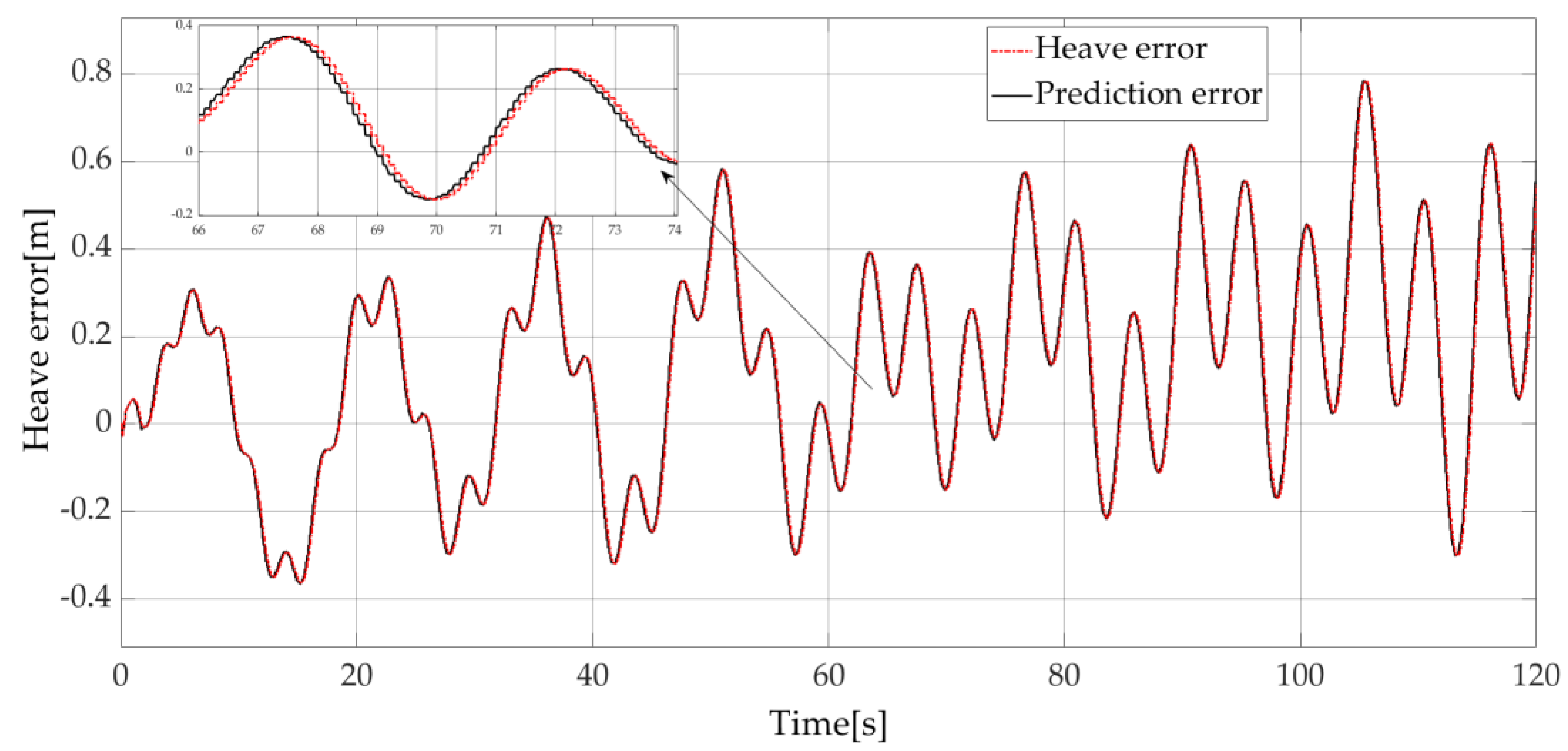
Using ARMA model for the prediction of the heave displacement, the reference value subtracts the actual value of position (the heave error) in the above Figure as the input signal of prediction. After using the above prediction method, the heave error and the prediction error are shown in Figure 11.

A zoom on the 66–74 s period for the predicted heave error results is shown in the top of Figure 11. These results show that ARMA models seem to be efficient tools for single-step prediction. These tools can be used efficiently for the compensating effect of the load’s movement and to reach a stable operation.

To objectively evaluate and analyze the performance of the different algorithms, the integral of the timeweighted absolute error (ITAE) is adopted in this paper. The performance criterion used is calculated by Equation (62):

$$\mathrm{J}={{\displaystyle \int }}_0^{\infty }\mathrm{t}\left|\mathrm{e}\left(\mathrm{t}\right)\right|\mathrm{dt}$$

(62)

where e(t) is the error between the reference and the obtained value of the controlled parameter, and t is the time (s).

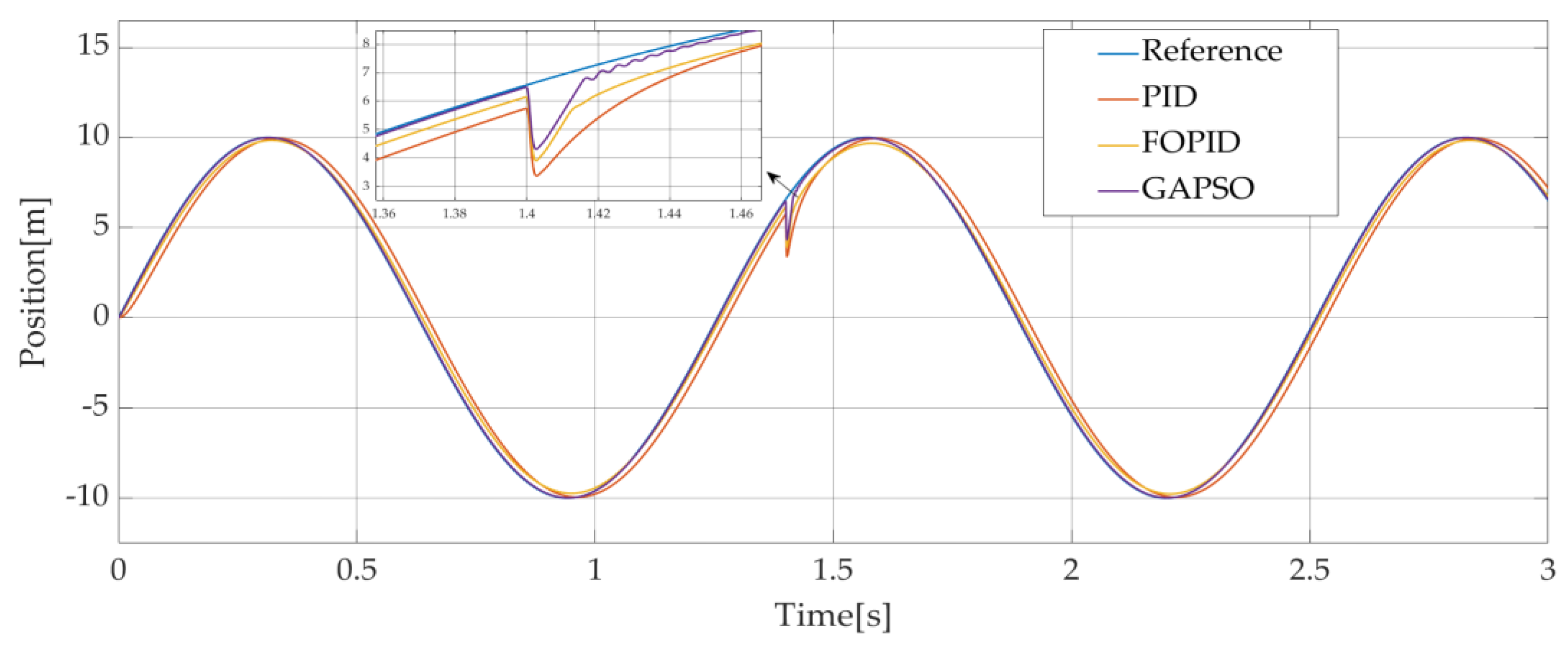
Figure 12 shows the results for different algorithms for the same reference signal for the position loop of PMSM. ASR and ACR use a PI controller. In this test case, only the PMSM is modeled. The input signal is set to a sinusoidal signal (Amplitude:10 m, frequency: 5 rad/s). A torque disturbance (with an amplitude of 400 N·m) is added at 1.4 s to observe the behavior of the position loop with different algorithms.

Simulation results presented in Figure 12 show that the fractional-order PID controller parameters adjusted using the GAPSO algorithm have the lowest ITAE metric and the best steady state performance during operation. It is minimally affected by disturbances and can be returned to a stable position very quickly. The ITAE metrics above are shown in

Table 4. ITAE metrics for each algorithm for the results of Figure 12.

Algorithms	ITAE
PID	5.4437
FOPID	2.3731
GAPSO	0.3024

:

4.1. Simulation When the Initial Rope Length L = 5 m and Fixed Position for the Load (V = 0 m/s)

A wave disturbance force is applied to the vessel and indirectly transferred to the crane load. The whole system is simulated using the system parameters and simulation conditions presented in Table 3.

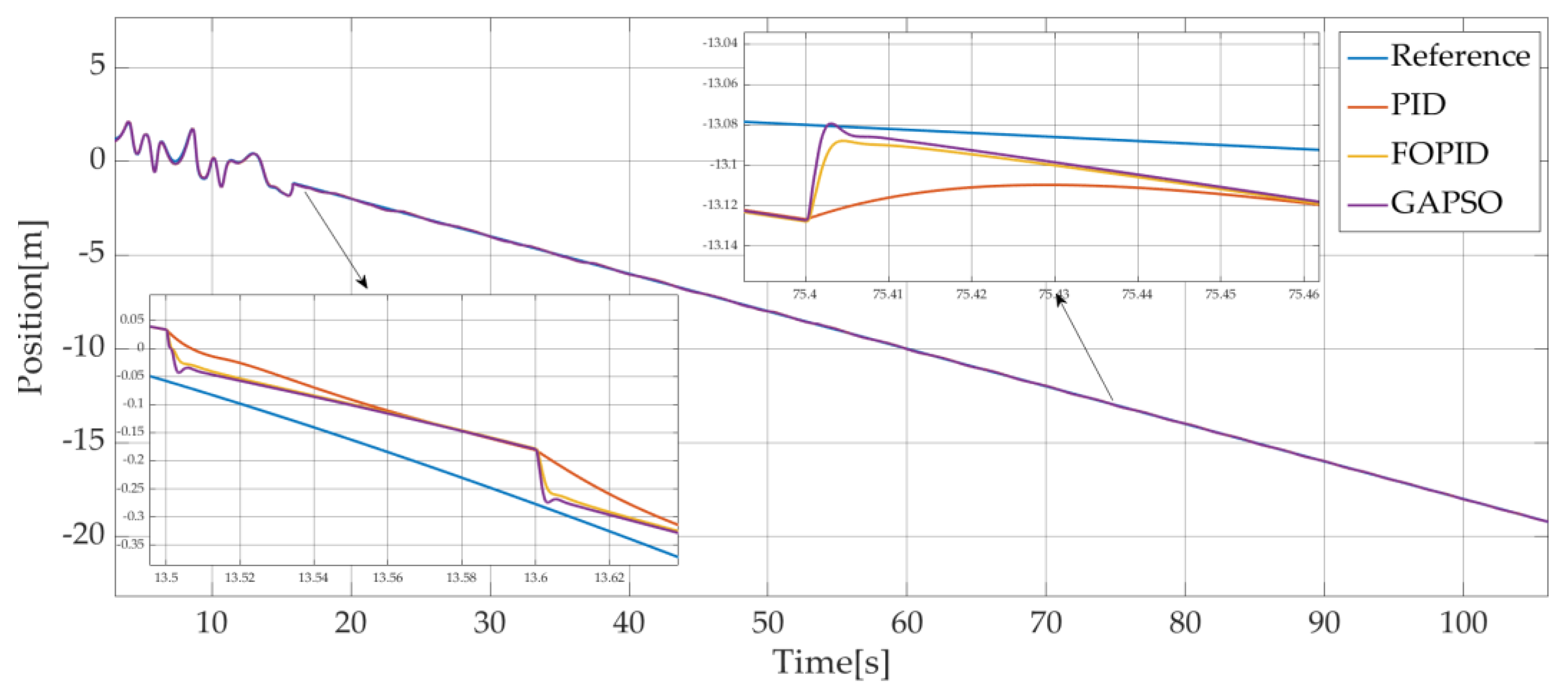
A first simulation is done with a rope length L = 5 m and a fixed reference position for the load (V = 0 m/s). A comparison of the position response of the different algorithms is shown in Figure 13:

As can be seen in Figure 12 and Figure 13 and

Table 5. Compensation efficiency of different algorithms using results of Figure 13.

Algorithms	η
PID	96.432%
FOPID	96.949%
GAPSO	97.369%

, the GAPSO algorithm has the best response curve among the above algorithms. A compensation efficiency indicator is used to evaluate the compensation effect.

The compensation efficiency indicator is calculated using the integral of the heave errors over time with and without compensation:

$$\mathsf{\eta }=1-\frac{{{\displaystyle \int }}_0^{\mathrm{t}}\left|{\mathrm{e}}_{1\left(\mathrm{t}\right)}\right|\mathrm{dt}}{{{\displaystyle \int }}_0^{\mathrm{t}}\left|{\mathrm{e}}_{2\left(\mathrm{t}\right)}\right|\mathrm{dt}}\times 100\%$$

(63)

where e₁(t) is the compensated heave error; e₂(t) is the heave error without the compensation.

As shown in Figure 14, the load will deviate from the reference position due to wave disturbance forces, a large heave error is generated in the vertical direction. However, with the action of the compensation motor, the heave error is greatly reduced after compensation. The compensation efficiencies (calculated by Equation (63)) are given in Table 5.

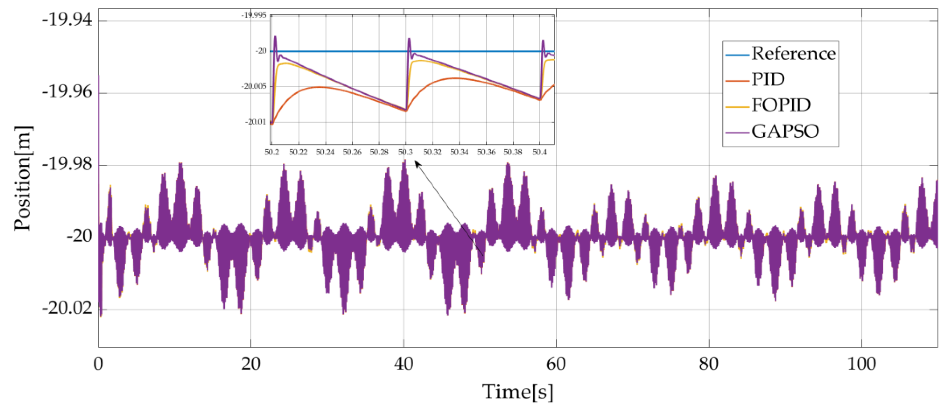
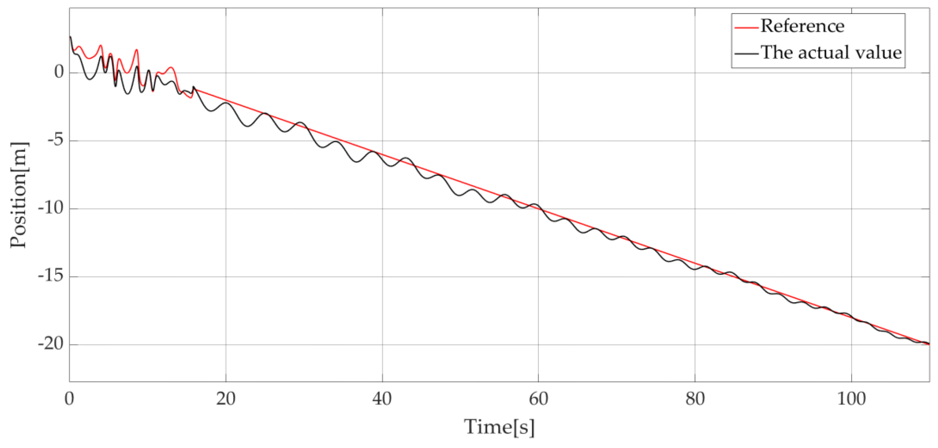
4.2. Simulation When the Initial Rope Length L = 5 m and the Lowering Speed of the Rope V = 0.2 m/s

In a second simulation, a descending speed of V = 0.2 m/s and an initial rope length equal to V = 5 m are considered with the same system parameters and environmental conditions than in subsection A, the simulation time is set to 110 s. Considering the effect of wave height, the load finally encountered the sea surface at approximately 96 s. The position of the load without compensation is shown in Figure 15 and the position of the load with compensation is shown in Figure 16.

As can be seen in the Figure 15 and Figure 16, the load essentially descends in accordance with the reference position if compensation is used. After 96 s, the load is under the sea surface and the sea surface height is added to the reference position of the load to prevent the rope from breaking suddenly (wave synchronization control strategy) [30]. This is why the reference position of the load becomes an irregular curve. 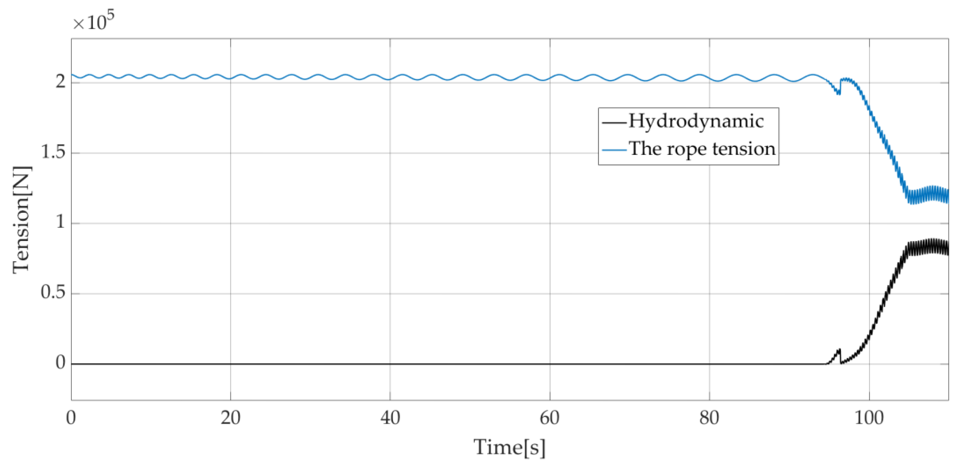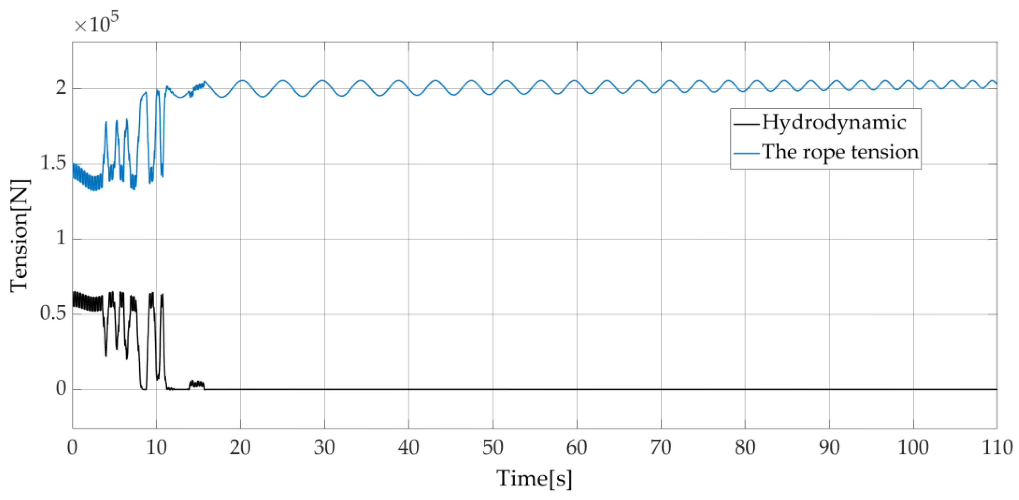Figure 17 and Figure 18 present rope tension and hydrodynamic forces on the load without and with wave synchronization strategy, respectively. From Figure 17, when the load is not in contact with the water, the hydrodynamic force is zero. After 96 s when the load is in contact with the water, the water will produce an upward impact on the load and buoyancy to reduce the tension of the rope. When the wave synchronizations control strategy is used, the tension of the rope, shown in Figure 18, is significantly reduced compared to Figure 17. This wave synchronization strategy allows for prevention of the rope breaking suddenly during operation.

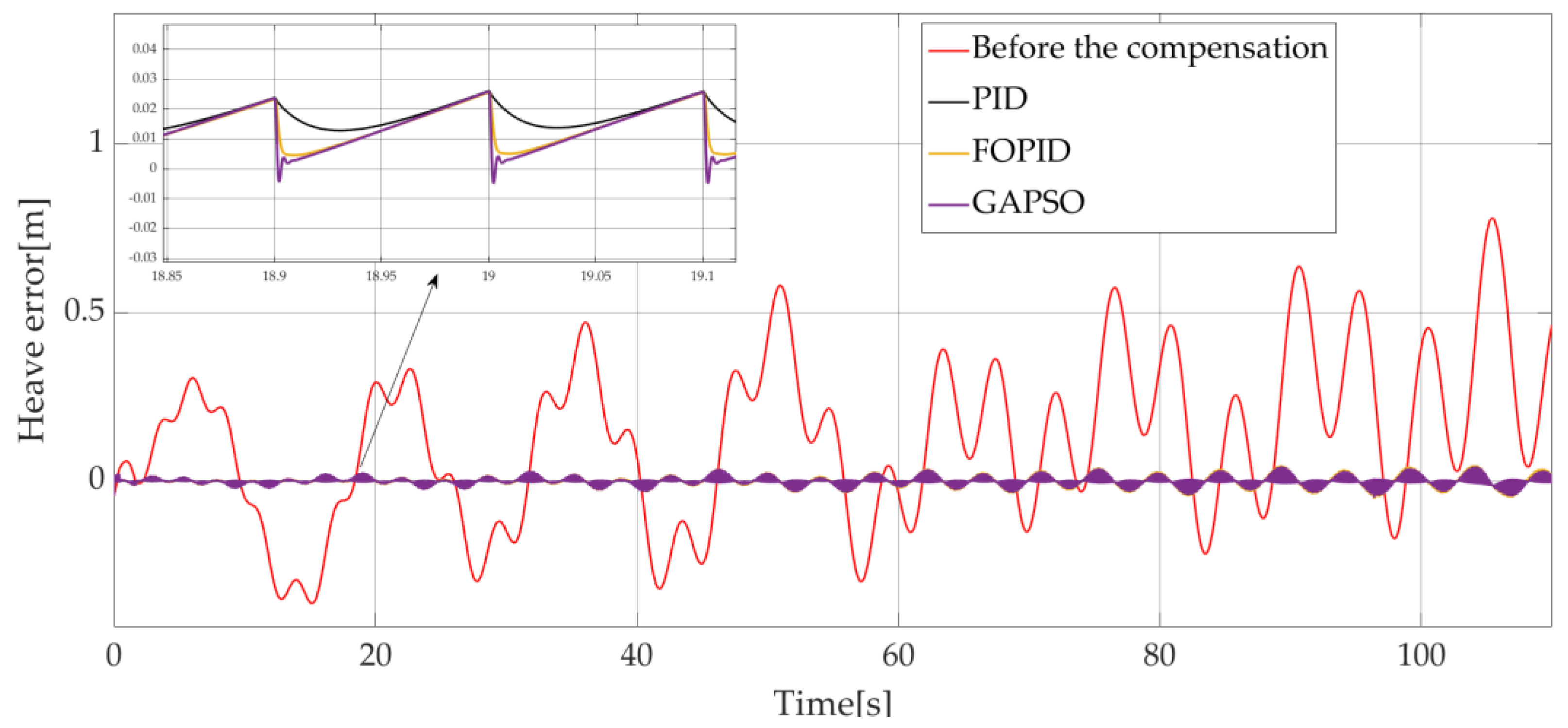
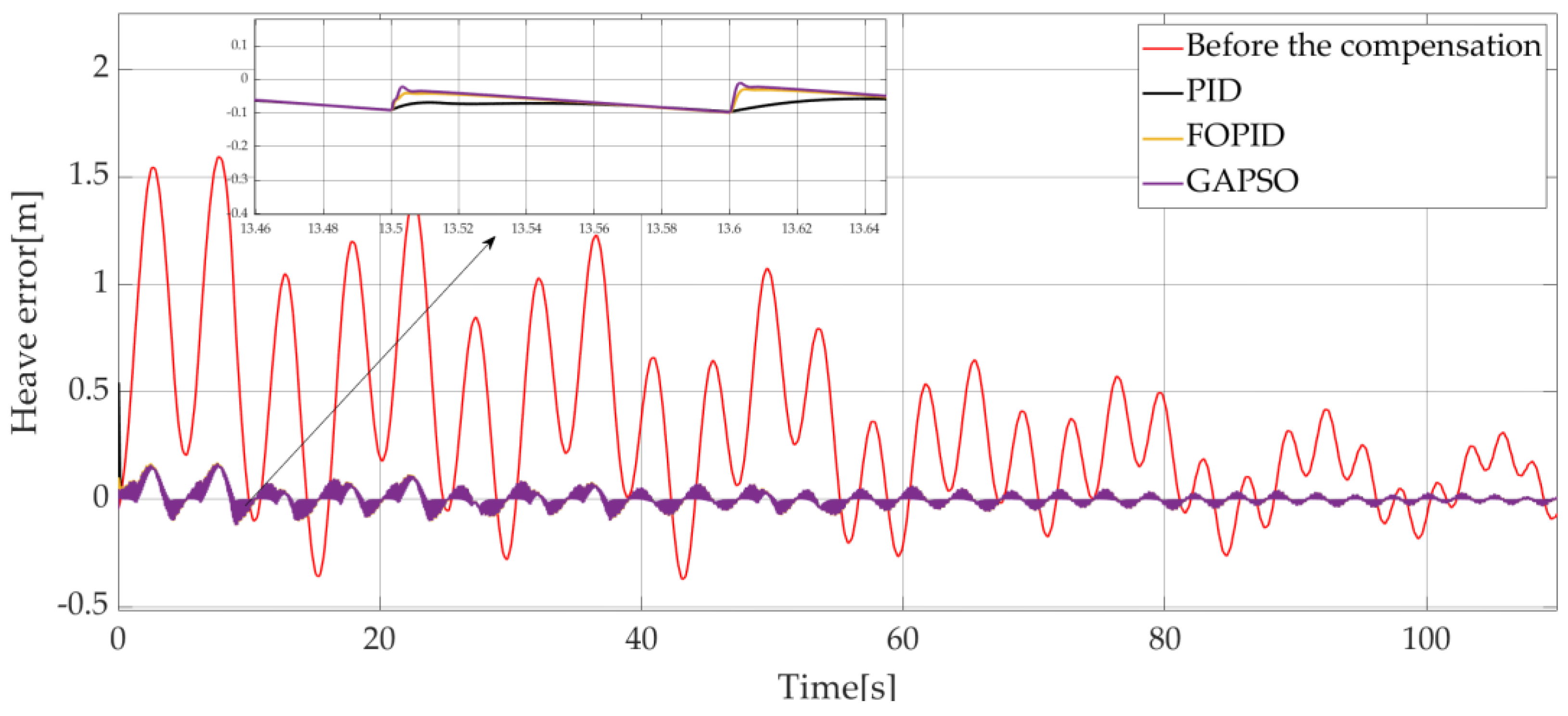
In the studied case, as shown in Figure 19 (which presents the heave errors) and

Table 6. Compensation efficiency for different algorithms using results of Figure 19.

Algorithms	η
PID	96.773%
FOPID	95.268%
GAPSO	96.135%

(which presents the compensation efficiencies for the different studied methods), PMSM with fractional-order PID controller tuned by GAPSO allows for a better compensation control than other methods.

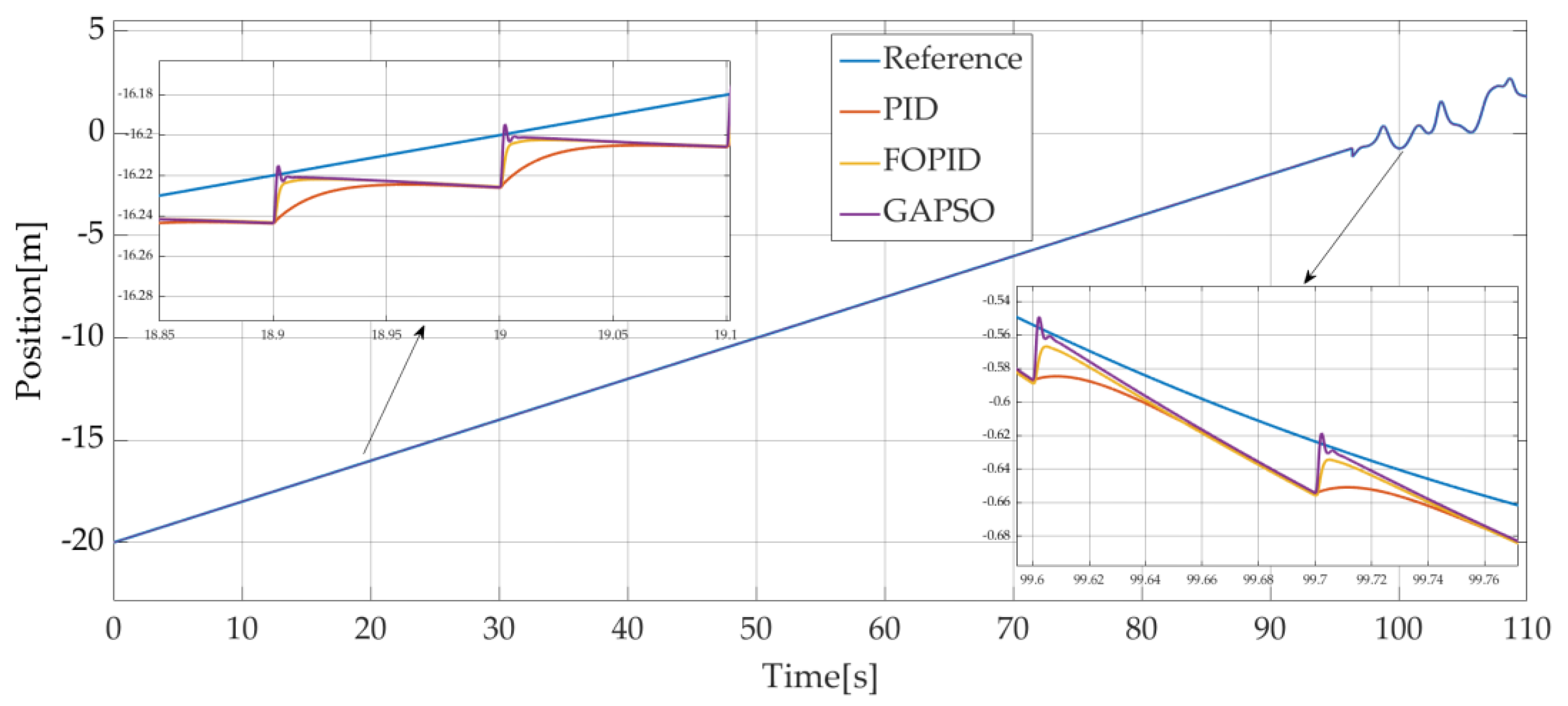
4.3. Simulation When the Initial Rope Length L = 27 m and the Rising Speed of the Rope of 0.2 m/s

In a third studied case, the initial rope length is set to 27 m, the load is submerged 2 m below sea level before rising at a speed of 0.2 m/s. Considering the effect of wave height, the load passes through the sea surface at roughly 15 s. A wave synchronization control strategy is added before t = 15 s when the load is in the contact with the sea. The simulation time was set to 110 s. The position of the load without compensation is shown in Figure 20 and the position of the load with compensation is shown in Figure 21.

The diagram shows that the longer the starting rope length, the more violent the swaying of the rope, resulting in significant heave errors. As the rope length is gradually shortened during operation, the swaying of the rope becomes progressively smaller. When a compensation control is used, the load can basically rise in accordance with the reference position.

The position of the load without and with compensation with the studied methods is shown in Figure 2. The corresponding heave errors are shown in Figure 22. And

Table 7. Compensation efficiency for different algorithms and the results of Figure 22.

Algorithms	η
PID	92.426%
FOPID	93.607%
GAPSO	94.068%

shows the compensation efficiency of the third study case.

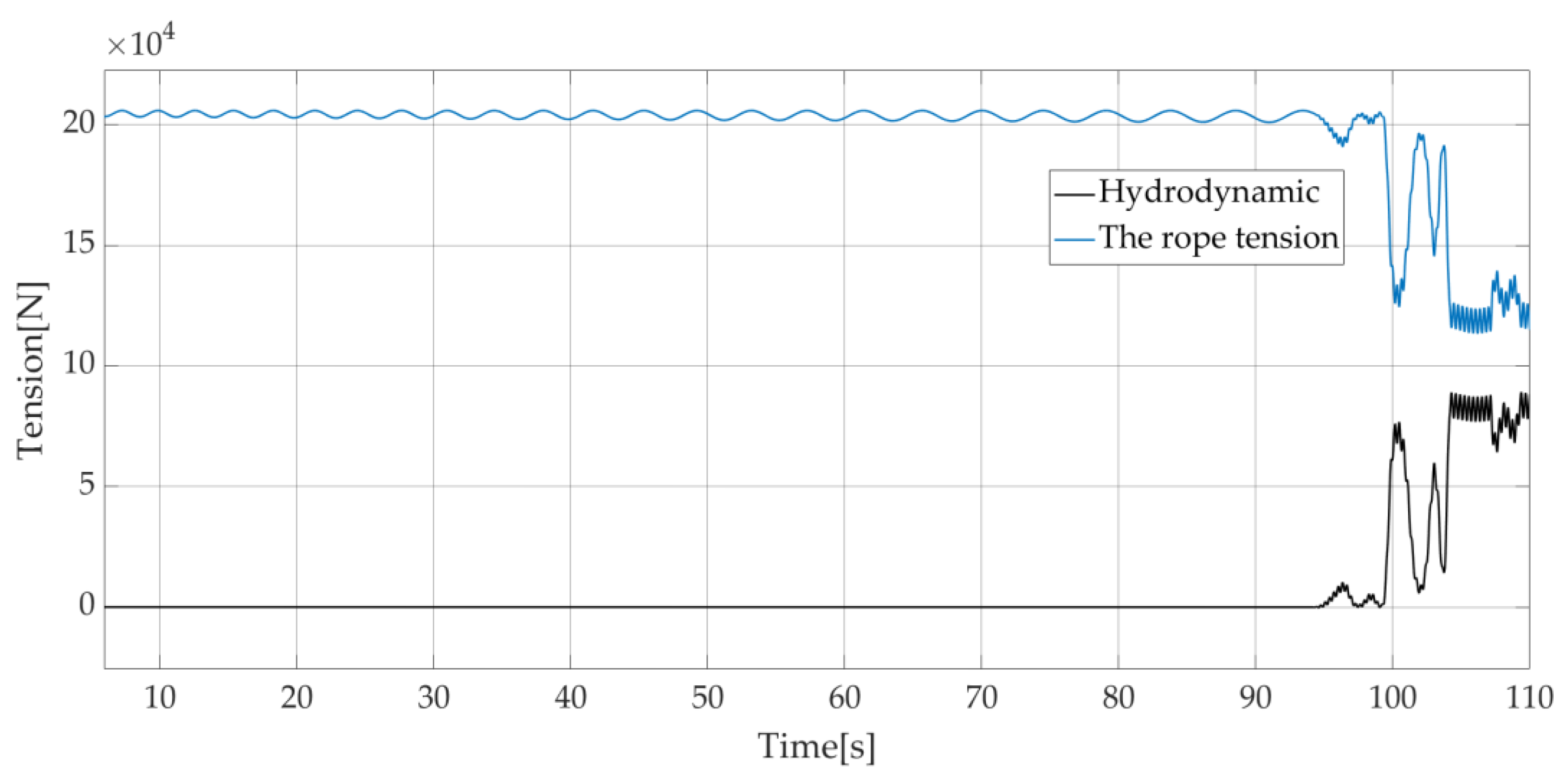
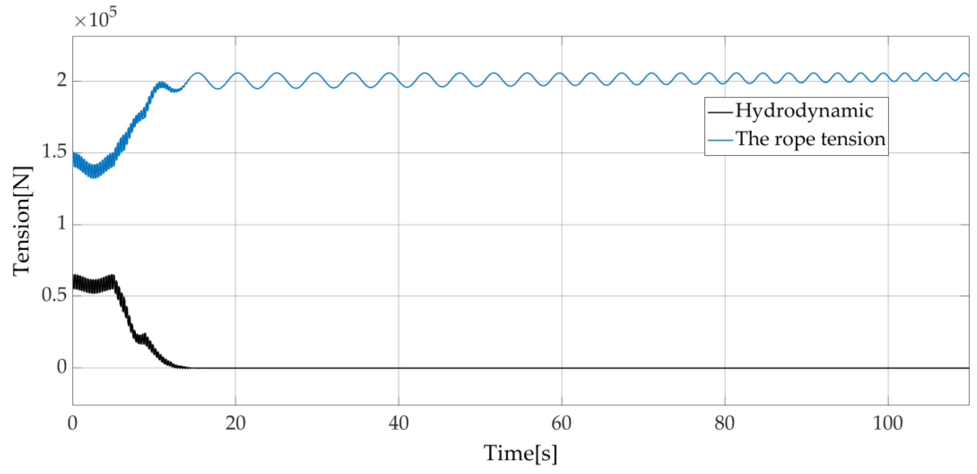
The evolution of the rope tension with and without the wave synchronization control strategy is shown in Figure 23 and Figure 24. As in the previous case (subsection B), it is shown that the wave synchronization control strategy can limit significantly the rope tension.

As a synthesis the presented results show the efficiency of the proposed methods for a better tracking of the load position in all the studied cases. The heave error is strongly reduced by the proposed GAPSO/FOPID compensation control strategy.

The wave synchronizations strategy can also make the rope tension change smoothly when entering or leaving the water, which is important for the actual work of the vessel in the sea.

5. Conclusions

An efficient strategy is proposed for wave compensation on a ship crane. This strategy associates a fractional-order PID based on a controller for the PMSM motor used for wave compensation in the crane system. A combined particle swarm and genetic algorithm is used to improve the parameters of the proposed controller. A wave synchronization strategy with reasonable prediction of heave displacements of the load is also used and proposed. In order to validate the proposed strategy, the overall structure of the system has been simulated in a MATLAB/Simulink environment. This whole model includes ship motion model, mechanical model of the crane, wave model, and compensation motor and motor control model. This simulation tool allows for representing the whole system’s behavior with accuracy. Simulation results on representative test cases show that the proposed approach is able to significantly improve the behavior of the system compared with more classical methods.