
A Novel Acoustic Method for Cavitation Identification of Propeller


Abstract
:1. Introduction
2. Identification for Cavitation States of Propeller Based on CEEMDAN-RCMFDE and Hybrid Optimization SVM
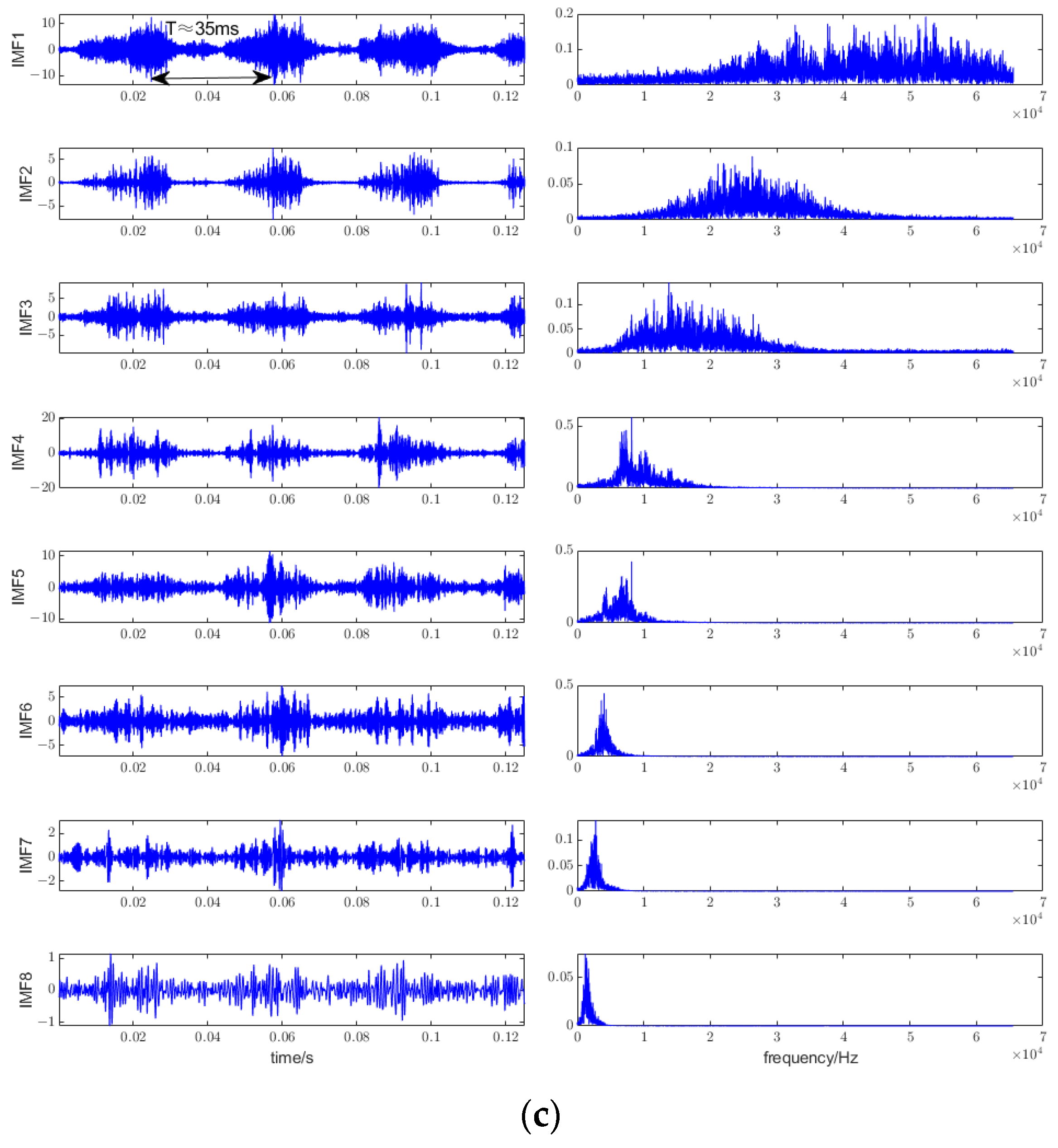
2.1. CEEMDAN Principle
2.2. RCMFDE Algorithm
2.2.1. FDE
2.2.2. RCMFDE
2.3. Hybrid Optimization SVM Classification Model
2.3.1. Relief-F
2.3.2. PSO Algorithm
2.3.3. Hybrid Optimization SVM Based on Relief-F and PSO
- (1)
- Use the Relief-F method to rank the features of the training sets from the highest best feature to the lowest using Equation (16).
- (2)
- Initialize parameters, including particle number, learning factor, weighting coefficient, particle position and particle velocity, and the penalty factor c and kernel parameter g of SVM are encoded as the position of the particle.
- (3)
- Train SVM model with the training set. The parameters c and g vary as the particle travels.
- (4)
- Assess the fitness values. The SVM corresponding to each particle is used to predict the training sample, and the prediction error of the current particle is taken as the fitness of the particle.
- (5)
- Determine whether the termination condition is satisfied. If the set ideal accuracy rate or number of iterations is attained, the iteration is discontinued. Otherwise, update the velocity and position of the particle swarm and resume step 3 to 5.
- (6)
- Load optimal parameters acquired to model and classify the test set.
2.4. Steps of Cavitation State Identification for Propeller Noise Signal
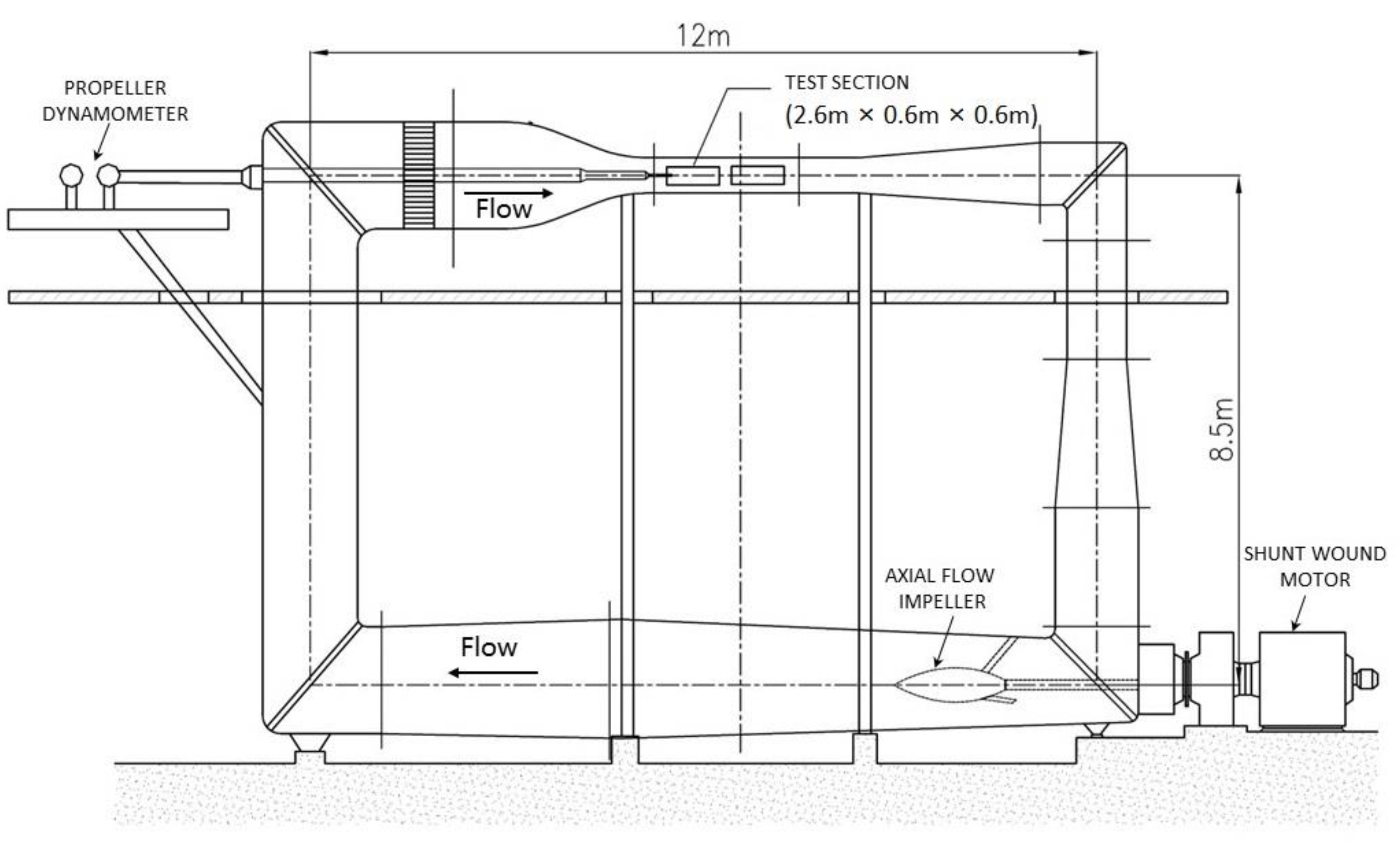
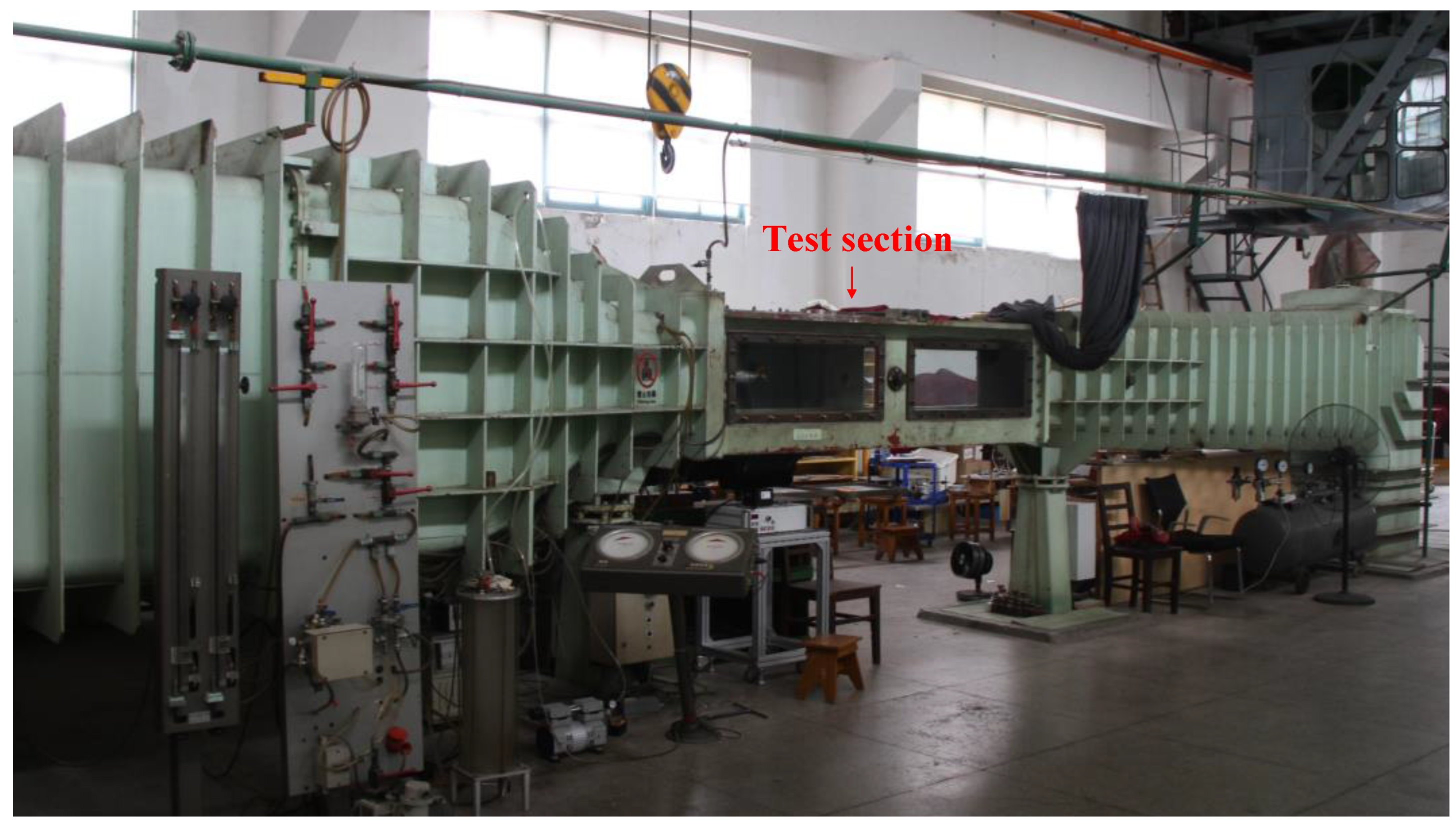
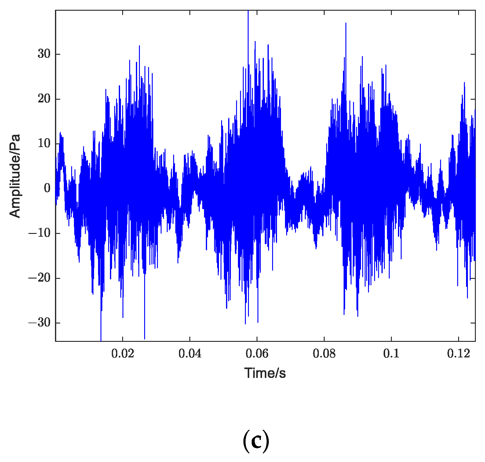
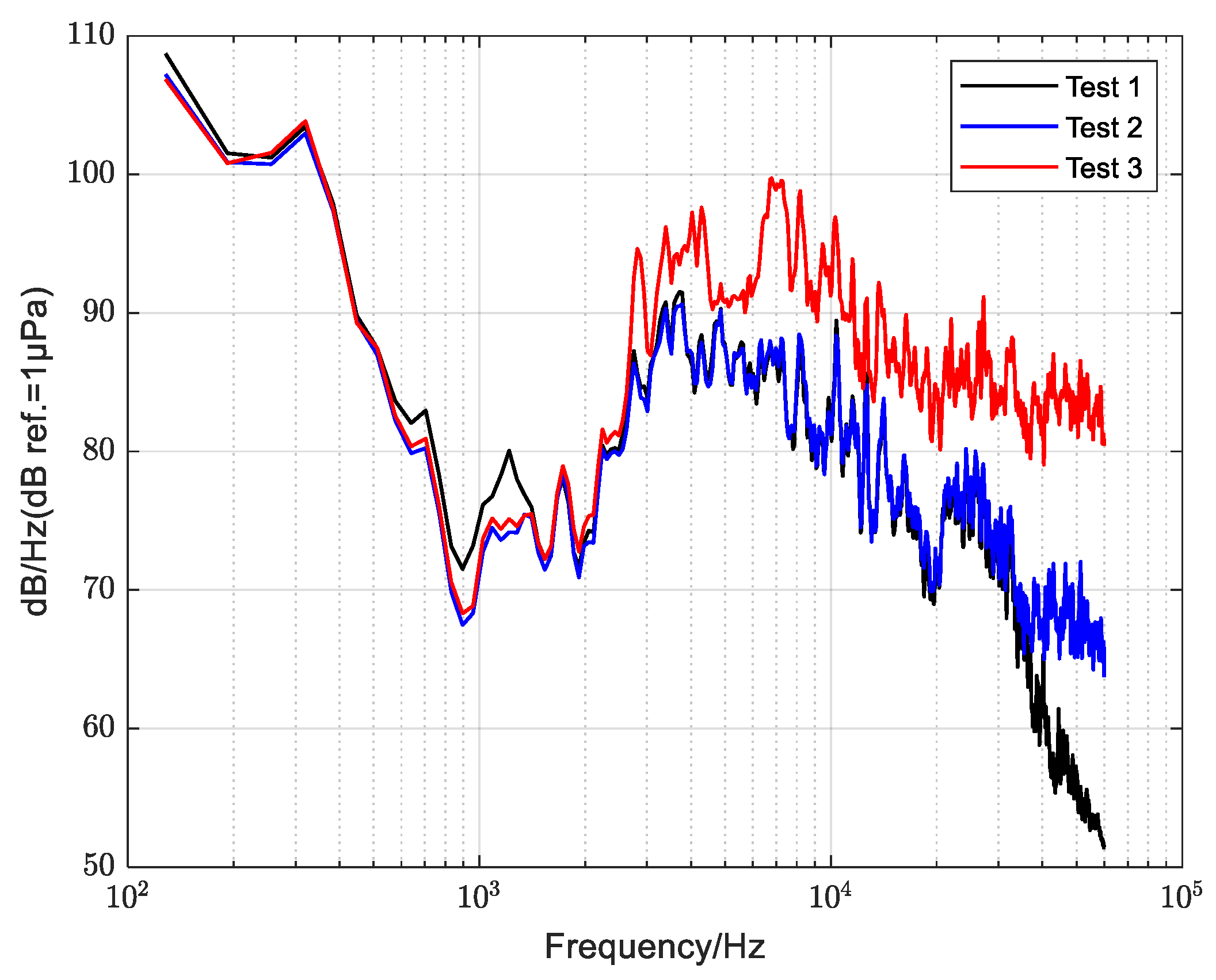
3. Experimental Investigation
4. Result and Discussion
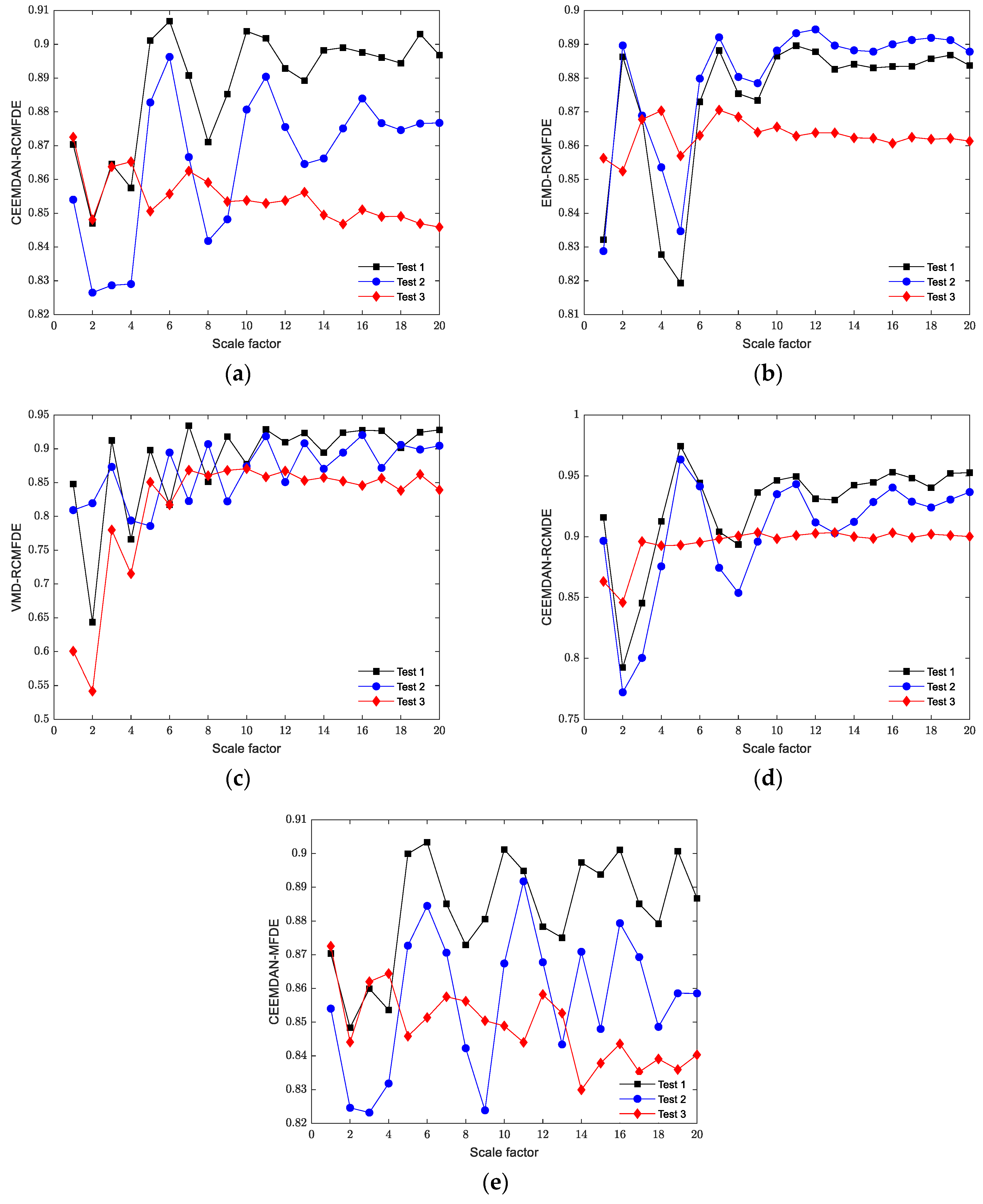
4.1. Cavitation Feature Extraction by CEEMDAN-RCMRDE
4.2. Diagnosis Results and Analysis
4.3. Comparison with Other Methods
5. Conclusions
Author Contributions
Funding
Institutional Review Board Statement
Informed Consent Statement
Data Availability Statement
Conflicts of Interest
Abbreviations
| RCMFDE | refined composite multiscale fluctuation-based dispersion entropy |
| CEEMDAN | complete ensemble empirical mode decomposition with adaptive noise |
| IMF | intrinsic mode function |
| SVM | support vector machine |
| PSO | particle swarm optimization |
| CIS | cavitation inception speed |
| STFT | short-time Fourier transform |
| WVD | Wigner-Ville distribution |
| TSA | time-domain synchronous averaging |
| EMD | empirical mode decomposition |
| FDE | fluctuation-based dispersion entropy |
| BPNN | back propagation neural networks |
| RF | random forest |
| EEMD | ensemble empirical mode decomposition |
| TVC | tip vortex cavitation |
| VMD | variational mode decomposition |
| RCMDE | refined composite multiscale dispersion entropy |
| MFDE | multiscale dispersion entropy |
| LS | Laplace score |
References
- Carlton, J.S. Chapter 9—Cavitation. In Marine Propellers and Propulsion, 4th ed.; Carlton, J.S., Ed.; Butterworth-Heinemann: Oxford, UK, 2019; pp. 217–260. [Google Scholar]
- Kuiper, G.; Jessup, S.D.; Bose, N.; Scherer, O.; Platzer, G.; Perez-Gomez, G. A propeller design method for unsteady conditions. Discussion. Authors’ closure. Trans.-Soc. Nav. Archit. Mar. Eng. 1993, 101, 247–273. [Google Scholar]
- Chang, Y.-C.; Hu, C.-N.; Tu, J.-C.; Chow, Y.-C. Experimental investigation and numerical prediction of cavitation incurred on propeller surfaces. J. Hydrodyn. 2010, 22, 722–727. [Google Scholar] [CrossRef]
- Aktas, B.; Atlar, M.; Turkmen, S.; Shi, W.; Sampson, R.; Korkut, E.; Fitzsimmons, P. Propeller cavitation noise investigations of a research vessel using medium size cavitation tunnel tests and full-scale trials. Ocean Eng. 2016, 120, 122–135. [Google Scholar] [CrossRef]
- Chen, L.; Zhang, L.; Peng, X.; Shao, X. Influence of water quality on the tip vortex cavitation inception. Phys. Fluids 2019, 31, 023303. [Google Scholar] [CrossRef]
- Lee, J.-H.; Han, J.-M.; Park, H.-G.; Seo, J.-S. Application of signal processing techniques to the detection of tip vortex cavitation noise in marine propeller. J. Hydrodyn. 2013, 25, 440–449. [Google Scholar] [CrossRef]
- He, Y.; Liu, Y. Experimental research into time–frequency characteristics of cavitation noise using wavelet scalogram. Appl. Acoust. 2011, 72, 721–731. [Google Scholar] [CrossRef]
- Dong, L.; Wu, K.; Zhu, J.-c.; Dai, C.; Zhang, L.-X.; Guo, J.-N. Cavitation detection in centrifugal pump based on interior flow-borne noise using WPD-PCA-RBF. Shock Vib. 2019, 2019, 8768043. [Google Scholar] [CrossRef]
- Widjiati, E.; Djatmiko, E.B.; Wardhana, W.; Wirawan. Analysis of propeller cavitation-induced signal using neural network and wigner-ville distribution. In Proceedings of the IEEE Oceans 2012, Yeosu, Korea, 21–24 May 2012; pp. 1–9. [Google Scholar]
- Wu, K.; Xing, Y.; Chu, N.; Wu, P.; Cao, L.; Wu, D. A carrier wave extraction method for cavitation characterization based on time synchronous average and time-frequency analysis. J. Sound Vib. 2020, 489, 115682. [Google Scholar] [CrossRef]
- Azizi, R.; Attaran, B.; Hajnayeb, A.; Ghanbarzadeh, A.; Changizian, M. Improving accuracy of cavitation severity detection in centrifugal pumps using a hybrid feature selection technique. Measurement 2017, 108, 9–17. [Google Scholar] [CrossRef]
- Torres, M.E.; Colominas, M.A.; Schlotthauer, G.; Flandrin, P. A complete ensemble empirical mode decomposition with adaptive noise. In Proceedings of the 2011 IEEE International Conference on Acoustics, Speech and Signal Processing (ICASSP), Prague, Czech Republic, 22–27 May 2011; pp. 4144–4147. [Google Scholar]
- Chen, W.; Li, J.; Wang, Q.; Han, K. Fault feature extraction and diagnosis of rolling bearings based on wavelet thresholding denoising with CEEMDAN energy entropy and PSO-LSSVM. Measurement 2021, 172, 108901. [Google Scholar] [CrossRef]
- Yao, L.; Pan, Z. A new method based CEEMDAN for removal of baseline wander and powerline interference in ECG signals. Optik 2020, 223, 165566. [Google Scholar] [CrossRef]
- Gao, B.; Huang, X.; Shi, J.; Tai, Y.; Zhang, J. Hourly forecasting of solar irradiance based on CEEMDAN and multi-strategy CNN-LSTM neural networks. Renew. Energy 2020, 162, 1665–1683. [Google Scholar] [CrossRef]
- Battarra, M.; Mucchi, E. Incipient cavitation detection in external gear pumps by means of vibro-acoustic measurements. Measurement 2018, 129, 51–61. [Google Scholar] [CrossRef]
- Dong, L.; Zhao, Y.; Dai, C. Detection of Inception Cavitation in Centrifugal Pump by Fluid-Borne Noise Diagnostic. Shock Vib. 2019, 2019, 9641478. [Google Scholar] [CrossRef]
- Lee, J.-H.; Seo, J.-S. Application of spectral kurtosis to the detection of tip vortex cavitation noise in marine propeller. Mech. Syst. Signal Process. 2013, 40, 222–236. [Google Scholar] [CrossRef]
- Song, Y.; Liu, J.; Wu, D.; Zhang, L. The MFBD: A novel weak features extraction method for rotating machinery. J. Braz. Soc. Mech. Sci. Eng. 2021, 43, 547. [Google Scholar] [CrossRef]
- Si, L.; Wang, Z.; Liu, X.; Tan, C. A sensing identification method for shearer cutting state based on modified multi-scale fuzzy entropy and support vector machine. Eng. Appl. Artif. Intell. 2019, 78, 86–101. [Google Scholar] [CrossRef]
- Flood, M.W.; Grimm, B. EntropyHub: An open-source toolkit for entropic time series analysis. PLoS ONE 2021, 16, e0259448. [Google Scholar] [CrossRef] [PubMed]
- Li, Y.; Jiao, S.; Geng, B. Refined composite multiscale fluctuation-based dispersion Lempel–Ziv complexity for signal analysis. ISA Trans. 2022, in press. [Google Scholar] [CrossRef]
- Zhou, F.; Gong, J.; Yang, X.; Han, T.; Yu, Z. A new gear intelligent fault diagnosis method based on refined composite hierarchical fluctuation dispersion entropy and manifold learning. Measurement 2021, 186, 110136. [Google Scholar] [CrossRef]
- Costa, M.; Goldberger, A.L.; Peng, C.-K. Multiscale entropy analysis of complex physiologic time series. Phys. Rev. Lett. 2002, 89, 068102. [Google Scholar] [CrossRef] [PubMed] [Green Version]
- Wu, S.-D.; Wu, C.-W.; Lin, S.-G.; Wang, C.-C.; Lee, K.-Y. Time series analysis using composite multiscale entropy. Entropy 2013, 15, 1069–1084. [Google Scholar] [CrossRef]
- Wu, S.-D.; Wu, C.-W.; Lin, S.-G.; Lee, K.-Y.; Peng, C.-K. Analysis of complex time series using refined composite multiscale entropy. Phys. Lett. A 2014, 378, 1369–1374. [Google Scholar] [CrossRef]
- Ye, M.; Yan, X.; Jia, M. Rolling bearing fault diagnosis based on VMD-MPE and PSO-SVM. Entropy 2021, 23, 762. [Google Scholar] [CrossRef] [PubMed]
- Zheng, J.; Pan, H.; Yang, S.; Cheng, J. Generalized composite multiscale permutation entropy and Laplacian score based rolling bearing fault diagnosis. Mech. Syst. Signal Process. 2018, 99, 229–243. [Google Scholar] [CrossRef]
- Azami, H.; Escudero, J. Amplitude-and fluctuation-based dispersion entropy. Entropy 2018, 20, 210. [Google Scholar] [CrossRef] [PubMed]
- Rostaghi, M.; Azami, H. Dispersion entropy: A measure for time-series analysis. IEEE Signal Process. Lett. 2016, 23, 610–614. [Google Scholar] [CrossRef]
- Kononenko, I. Estimating attributes: Analysis and extensions of RELIEF. In Proceedings of the European Conference on Machine Learning on Machine Learning, Catania, Italy, 6–8 April 1994; Springer: Berlin/Heidelberg, Germany, 1994. [Google Scholar]
- Tang, F.; Chen, M.; Wang, Z. New approach to training support vector machine. J. Syst. Eng. Electron. 2006, 17, 200–219. [Google Scholar]
- Zhang, L.; Wu, D.; Han, X.; Zhu, Z. Feature Extraction of Underwater Target Signal Using Mel Frequency Cepstrum Coefficients Based on Acoustic Vector Sensor. J. Sens. 2016, 2016, 7864213. [Google Scholar] [CrossRef] [Green Version]
- He, X.; Deng, C.; Niyogi, P. Laplacian Score for Feature Selection. In Proceedings of the Advances in Neural Information Processing Systems 18, Vancouver, BC, Canada, 5–8 December 2005. [Google Scholar]


| Item | Value |
|---|---|
| Dimension of test section, length × width × height | 2.6 m × 0.6 m × 0.6 m |
| Pressure range | 10~200 kPa |
| Maximum velocity | 12 m/s |
| Velocity instability | ≤1% |
| Velocity unevenness | ≤1% |
| Minimum cavitation number | 0.2 |
| Motor capacity | 90 kW |
| Parameter | Value |
|---|---|
| Number of blades | 5 |
| Diameter | 180 mm |
| Pitch ratio | 1.2 |
| Area ratio | 0.725 |
| Boss ratio | 0.2 |
| Material | brass |
| Item | Model | Parameter |
|---|---|---|
| Hydrophone | B&K 8104 | Frequency range: 0.1 Hz–120 kHz Charge sensitivity: 0.44 pC/Pa |
| Charge-amplifier | B&K 2690A | Frequency range: 0–100 kHz |
| Data Acquisition System | B&K LAN-XI 3161 | Frequency range: 0–204.8 kHz |
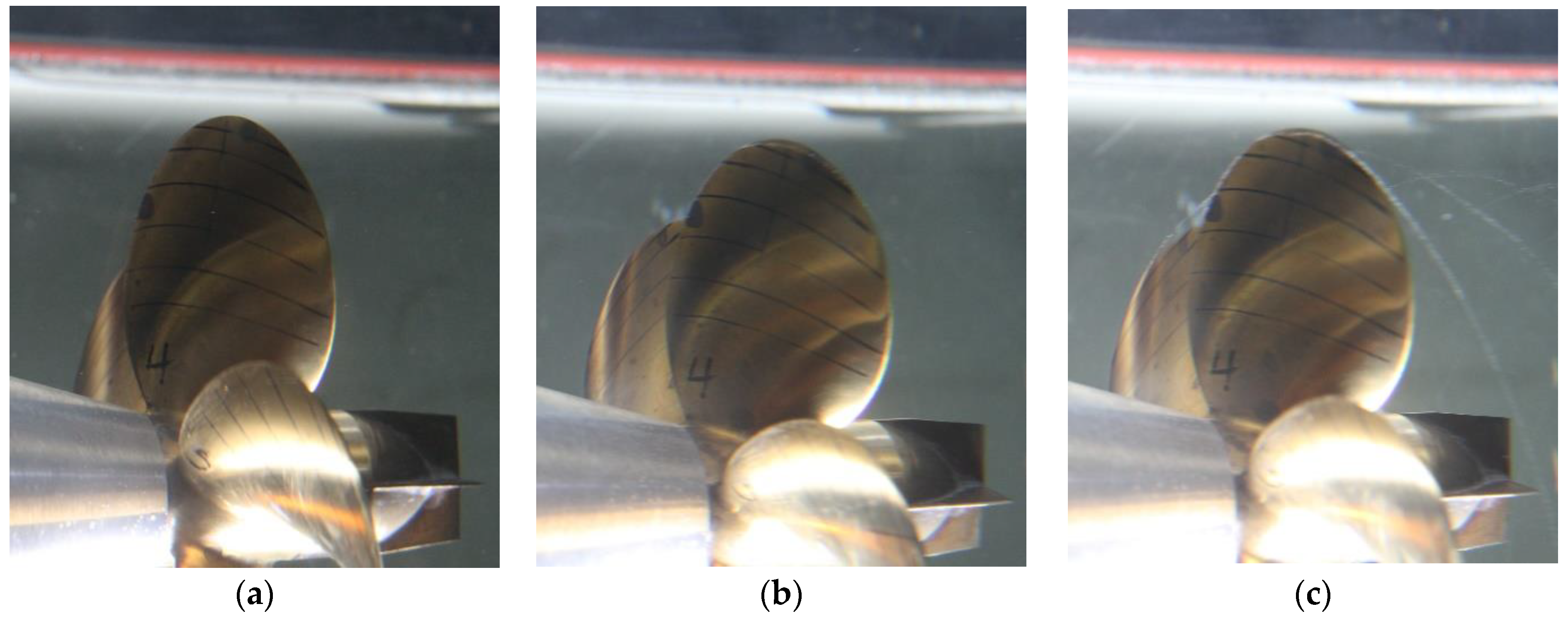
| Test Number | Pressure | Rotation Speed n/rps | Cavitation Number | Inflow Velocity V/m/s | Cavitation State | |
|---|---|---|---|---|---|---|
| 1 | 103.2 | 28 | 7.93 | 4.69 | 0.24 | No cavitation |
| 2 | 3.54 | 0.33 | Cavitation inception | |||
| 3 | 3.32 | 0.35 | Full cavitation |
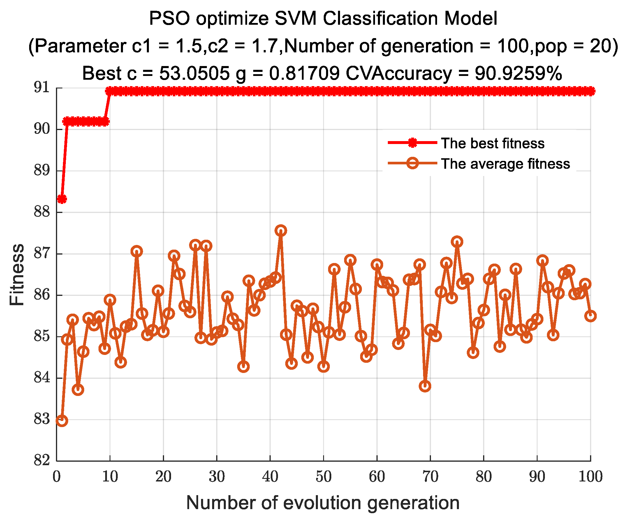
| G | N | c1 | c2 | w | c | g |
|---|---|---|---|---|---|---|
| 100 | 20 | 1.5 | 1.7 | 1 | [0.1, 100] | [0.1, 100] |
Publisher’s Note: MDPI stays neutral with regard to jurisdictional claims in published maps and institutional affiliations. |
© 2022 by the authors. Licensee MDPI, Basel, Switzerland. This article is an open access article distributed under the terms and conditions of the Creative Commons Attribution (CC BY) license (https://creativecommons.org/licenses/by/4.0/).
Share and Cite
Li, Y.; Cui, L. A Novel Acoustic Method for Cavitation Identification of Propeller. J. Mar. Sci. Eng. 2022, 10, 1225. https://doi.org/10.3390/jmse10091225
Li Y, Cui L. A Novel Acoustic Method for Cavitation Identification of Propeller. Journal of Marine Science and Engineering. 2022; 10(9):1225. https://doi.org/10.3390/jmse10091225
Chicago/Turabian StyleLi, Yang, and Lilin Cui. 2022. "A Novel Acoustic Method for Cavitation Identification of Propeller" Journal of Marine Science and Engineering 10, no. 9: 1225. https://doi.org/10.3390/jmse10091225
APA StyleLi, Y., & Cui, L. (2022). A Novel Acoustic Method for Cavitation Identification of Propeller. Journal of Marine Science and Engineering, 10(9), 1225. https://doi.org/10.3390/jmse10091225