
Study on Small Samples Active Sonar Target Recognition Based on Deep Learning

Abstract
:1. Introduction
- (1)
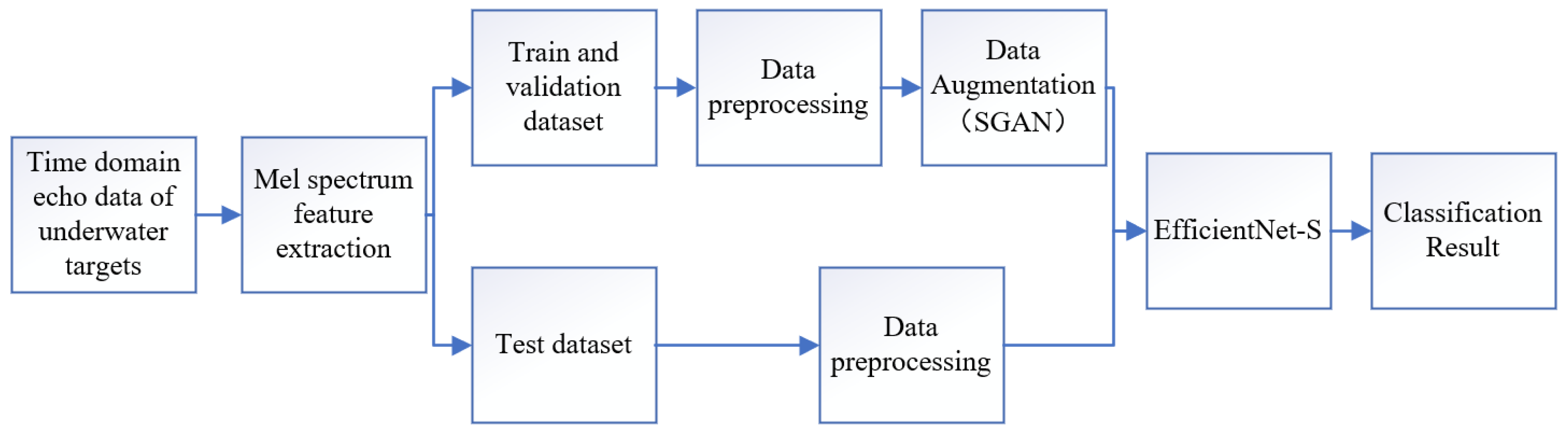
- We obtain Mel-spectrograms of the target’s echoes after Mel spectrum feature extraction. A novel network structure named EfficientNet-S is proposed to achieve higher recognition accuracy with small samples.
- (2)
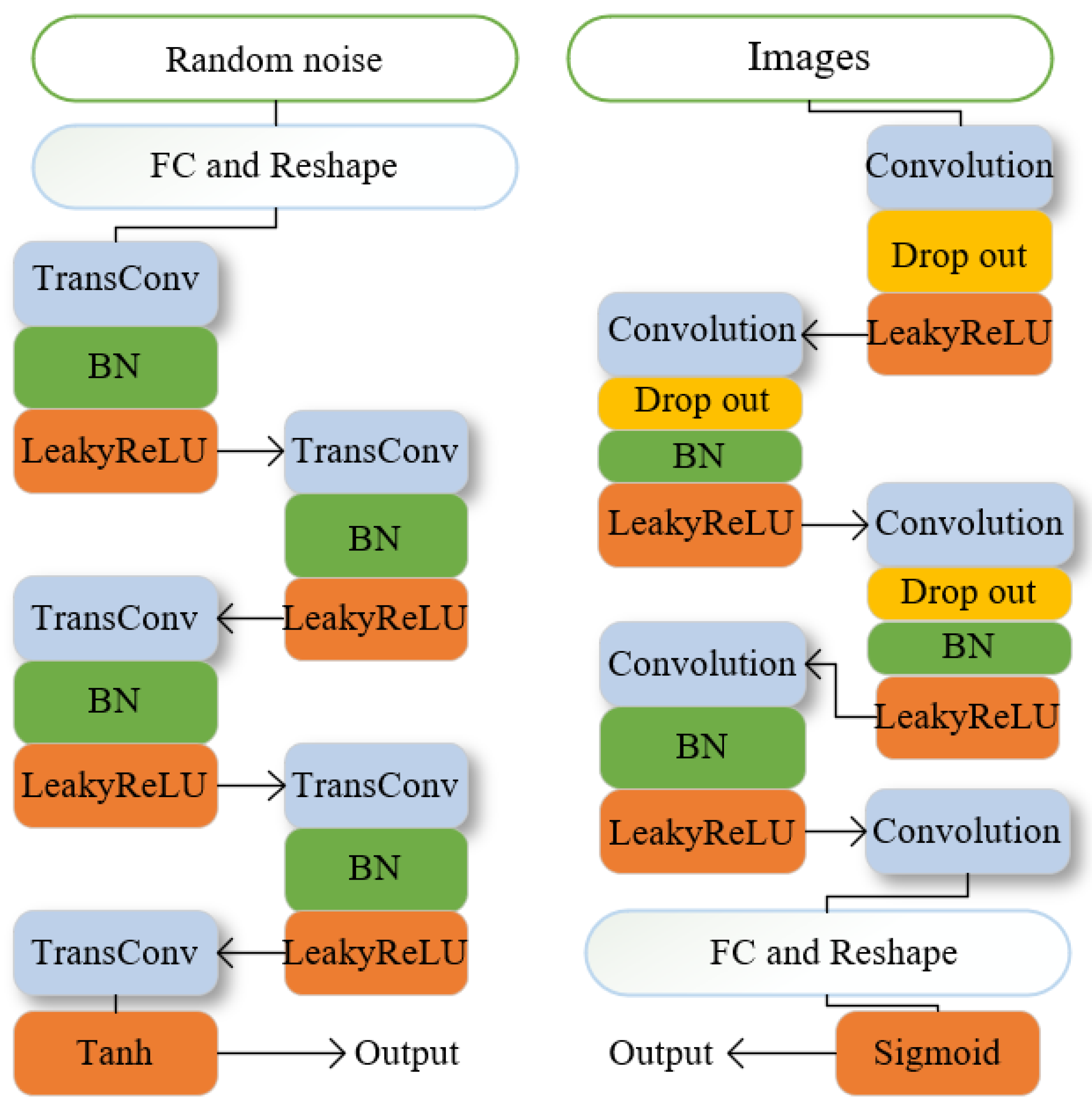
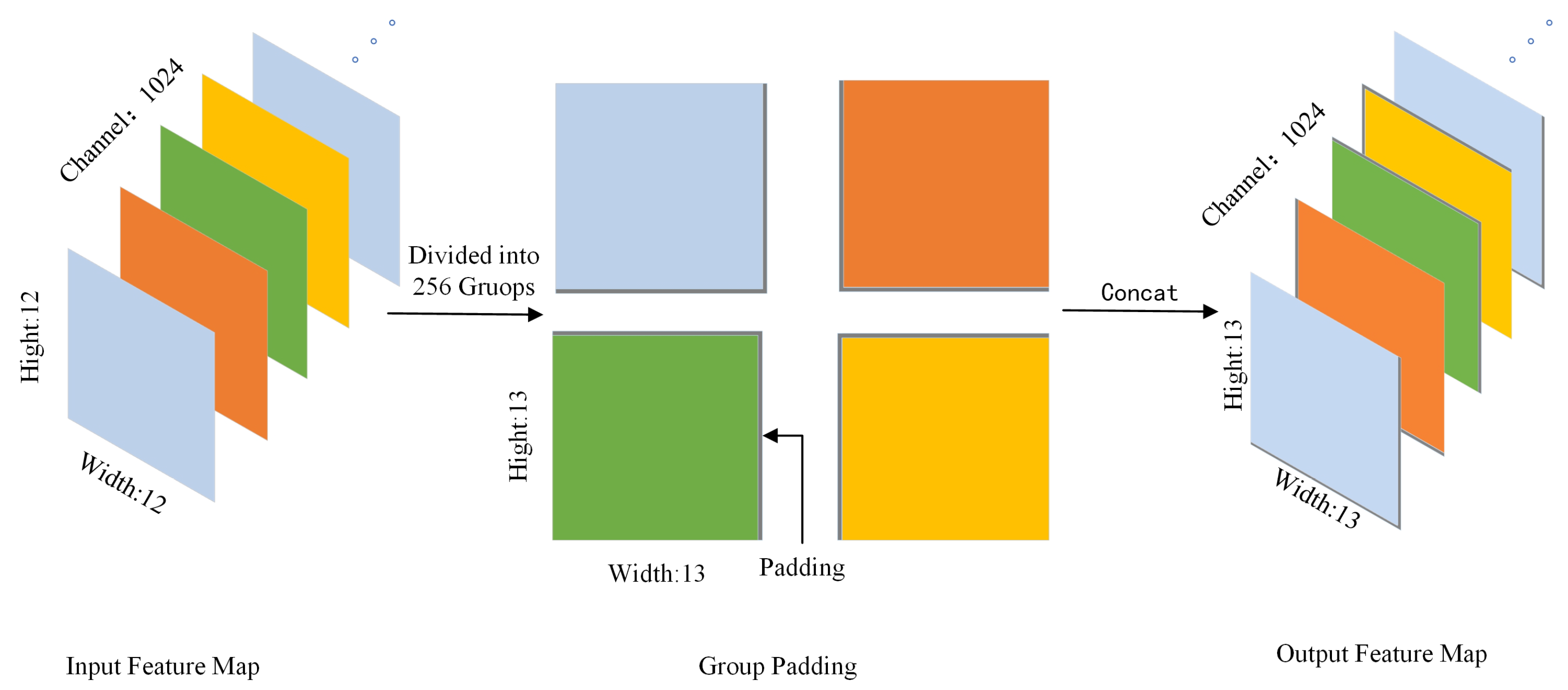
- We propose a novel generative adversarial network model (SGAN) model by combining group padding and even-sized convolution kernel. The simulation experiments show that the proposed method can efficiently generate high-quality time–frequency images.
- (3)
- We validate our algorithm on the anechoic pool experimental dataset. The result shows that it effectively solves the problem of insufficient accuracy faced with underwater target classification recognition in the case of small samples.
2. Methods
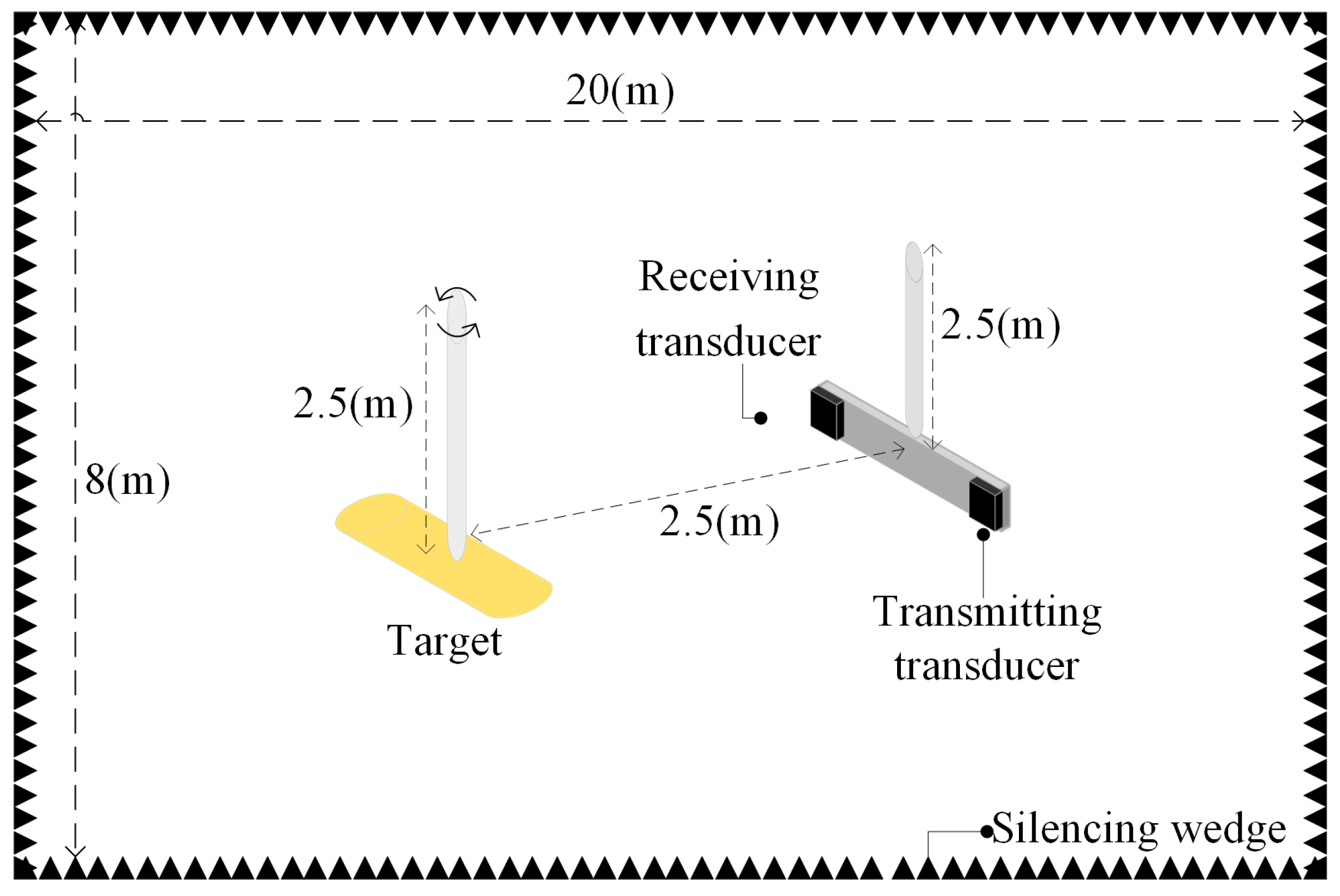
2.1. Setting up Dataset Based on Active Sonar Echoes
2.2. The Underwater Acoustic Target Recognition Method Based on Efficientnet
2.2.1. Baseline Model
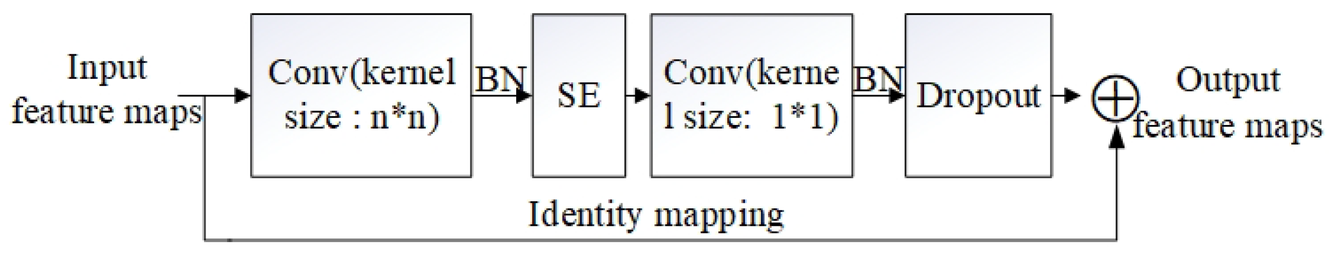
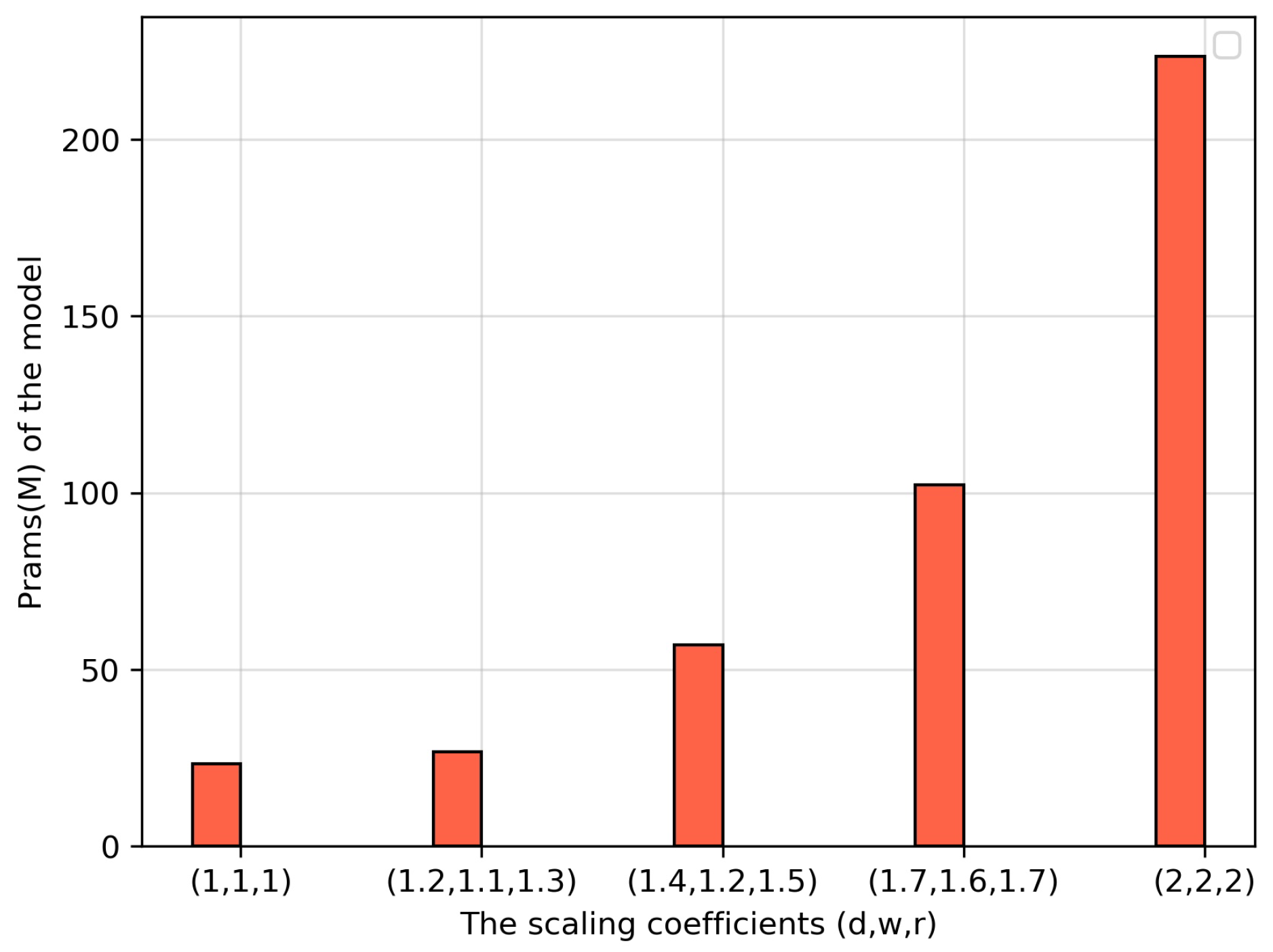
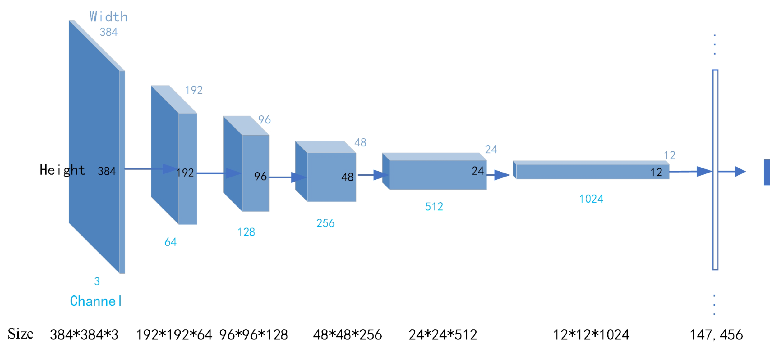
2.2.2. The Optimization Model (Efficientnet-S)
2.3. A Novel Generating Adversarial Networks
2.3.1. Principle of Generating Adversarial Network
2.3.2. Sgan Architecture
3. Experiment
3.1. Experimental Dataset
3.2. Model Evaluation Metrics
3.3. Result Analysis
4. Discussion
5. Conclusions
Author Contributions
Funding
Institutional Review Board Statement
Informed Consent Statement
Data Availability Statement
Conflicts of Interest
References
- Li, X.; Wu, Y. The classification of spherical shells with varying thickness-to-radius ratios based on the auditory perceptive features. J. Acoust. Soc. Am. 2019, 145, 1693. [Google Scholar] [CrossRef]
- Zou, L.; Ke, T.; Zha, J. Active sonar detection using adaptive time-frequency feature. In Proceedings of the 2016 IEEE/OES China Ocean Acoustics (COA), Haerbin, China, 9–11 January 2016. [Google Scholar]
- Hinton, G.E.; Salakhutdinov, R.R. Reducing the dimensionality of data with neural networks. Science 2006, 313, 504–507. [Google Scholar] [CrossRef] [PubMed]
- Yang, H.; Li, J.; Sheng, M. Underwater acoustic target multi-attribute correlation perception method based on deep learning. Appl. Acoust. 2022, 190, 108644. [Google Scholar]
- Zhang, T.; Feng, G.; Liang, J.; An, T. Acoustic scene classification based on Mel spectrogram decomposition and model merging. Appl. Acoust. 2021, 182, 108258. [Google Scholar] [CrossRef]
- Miao, Y.; Zakharov, Y.V.; Sun, H.; Li, J.; Wang, J. Underwater Acoustic Signal Classification Based on Sparse Time–Frequency Representation and Deep Learning. IEEE J. Ocean. Eng. 2021, 46, 952–962. [Google Scholar] [CrossRef]
- Lakshmi, M.D.; Santhanam, S.M. Underwater Image Recognition Detector using Deep ConvNet. In Proceedings of the 2020 National Conference on Communications (NCC), Kharagpur, India, 21–23 February 2020. [Google Scholar]
- Wei, Z.; Yang, J.; Min, S. A Method of Underwater Acoustic Signal Classification Based on Deep Neural Network. In Proceedings of the 2018 5th International Conference on Information Science and Control Engineering (ICISCE), Zhengzhou, China, 20–22 July 2018. [Google Scholar]
- Bu, M.; Benen, S.; Kraus, D. False Alarm Reduction for Active Sonars using Deep Learning Architectures. In Proceedings of the Undersea Defence Technology (UDT), Stockholm, Sweden, 15 May 2019. [Google Scholar]
- Lee, S.; Seo, I.; Seok, J. Active Sonar Target Classification with Power-Normalized Cepstral Coefficients and Convolutional Neural Network. Appl. Sci. 2020, 10, 8450. [Google Scholar] [CrossRef]
- Berg, H.; Hjelmervik, K.T. Deep Learning on Active Sonar Data Using Bayesian Optimization for Hyperparameter Tuning. In Proceedings of the 2020 25th International Conference on Pattern Recognition (ICPR), Milan, Italy, 10–15 January 2021. [Google Scholar]
- Feifei, L.; Fergus, R.; Perona, P. One-shot learning of object categories. IEEE Trans. Pattern. Anal. Mach. Intell. 2006, 28, 594–611. [Google Scholar] [CrossRef] [PubMed]
- Berg, H.; Hjelmervik, K.T. Classification of anti-submarine warfare sonar targets using a deep neural network. In Proceedings of the MTS/IEEE Charleston OCEANS Conference, Charleston, SC, USA, 22–25 October 2018. [Google Scholar]
- Wang, H.; Wang, B.; Li, Y. IAFNet: Few-Shot Learning for Modulation Recognition in Underwater Impulsive Noise. IEEE Commun. Lett. 2022, 26, 1047–1051. [Google Scholar] [CrossRef]
- Testolin, A.; Kipnis, D.; Diamant, R. Detecting Submerged Objects Using Active Acoustics and Deep Neural Networks: A Test Case for Pelagic Fish. Appl. Sci. 2020, 10, 2776–2788. [Google Scholar] [CrossRef]
- Sun, F.; Wang, M.; Xu, Q.; Xuan, X.; Zhang, X. Acoustic Scene Recognition Based on Convolutional Neural Networks. In Proceedings of the 2019 IEEE 4th International Conference on Signal and Image Processing (ICSIP), Wuxi, China, 19–21 July 2019. [Google Scholar]
- Tan, M.; Le, Q.V. EfficientNet: Rethinking model scaling for convolutional neural networks. arXiv 2019, arXiv:1905.11946. [Google Scholar]
- Tan, M.; Le, Q.V. EfficientNetV2: Smaller models and faster training. arXiv 2021, arXiv:2104.00298. [Google Scholar]
- Liu, Z.; Mao, H.; Wu, C.Y.; Feichtenhofer, C.; Darrell, T.; Xie, S. A ConvNet for the 2020s. In Proceedings of the IEEE/CVF Conference on Computer Vision and Pattern Recognition (CVPR), New Orleans, LA, USA, 19–23 June 2022. [Google Scholar]
- Goodfellow, I.J.; Pouget-Abadie, J.; Mirza, M.; Xu, B.; Warde-Farley, D.; Ozair, S.; Courville, A.; Bengio, Y. Generative adversarial nets. In Proceedings of the Neural Information Processing Systems, Montreal, QC, Canada, 8 December 2014. [Google Scholar]
- Radford, A.; Metz, L.; Chintala, S. Unsupervised Representation Learning with Deep Convolutional Generative Adversarial Networks. In Proceedings of the 4th International Conference on Learning Representations (ICLR 2016), San Juan, Puerto Rico, 2–4 May 2016. [Google Scholar]
- Wu, S.; Wang, G.; Tang, P.; Chen, F.; Shi, L. Convolution with even-sized kernels and symmetric padding. In Proceedings of the NeurIPS 2019, Vancouver, BC, Canada, 8–14 December 2019. [Google Scholar]
- Alain, H.; Ziou, D. Image quality metrics: PSNR vs. SSIM. In Proceedings of the 20th International Conference on Pattern Recognition, Istanbul, Turkey, 23–26 August 2010. [Google Scholar]


| Stage and Operator | Channels | Repetitions | |||
|---|---|---|---|---|---|
| Baseline model (B) and Efficientnet-S (S) | B | S | B | S | |
| 0 | Conv3×3 | 24 | 28 | 1 | 1 |
| 1 | Base-Conv, k7×7 | 24 | 28 | 1 | 1 |
| 2 | Base -Conv, k5×5 | 96 | 116 | 1 | 1 |
| 3 | Base -Conv, k3×3 | 384 | 460 | 2 | 3 |
| 4 | Base -Conv, k3×3, SE0.25 | 96 | 116 | 2 | 3 |
| 5 | Base -Conv, k3×3, SE0.25 | 128 | 154 | 3 | 4 |
| 6 | Base -Conv, k3×3, SE0.25 | 256 | 308 | 4 | 6 |
| 7 | Conv1×1 + Pooling + FC | 4 | 4 | 1 | 1 |
| Models | SNRs (dB) | Test Set Accuracy (%) |
|---|---|---|
| Baseline | 5 | 91.25 |
| Efficientnet-S | 5 | 96.25 |
| Baseline | 0 | 85.00 |
| Efficientnet-S | 0 | 91.25 |
| Baseline | −5 | 72.50 |
| Efficientnet-S | −5 | 77.50 |
| Baseline | −10 | 68.75 |
| Efficientnet-S | −10 | 73.75 |
| Categories | Train and val | Train and val (Expanded Number) | Test | Total | Total (Expanded Number) |
|---|---|---|---|---|---|
| Target 1 | 116 | 300 | 20 | 136 | 320 |
| Target 2 | 116 | 300 | 20 | 136 | 320 |
| Target 3 | 116 | 300 | 20 | 136 | 320 |
| Target 4 | 116 | 300 | 20 | 136 | 320 |
| Models | Scaling Factor d | Scaling Factor w | Scaling Factor r | Test Set Accuracy (%) | Training Time (s) |
|---|---|---|---|---|---|
| Baseline | 1 | 1 | 1 | 78.8 | 223.5 |
| Baseline | 1.2 | 1.1 | 1.3 | 86.3 | 422.7 |
| Baseline | 1.4 | 1.2 | 1.5 | 90.0 | 546.8 |
| Baseline | 1.7 | 1.6 | 1.7 | 85.0 | 1500.4 |
| Baseline | 2 | 2 | 2 | 83.8 | 2721.6 |
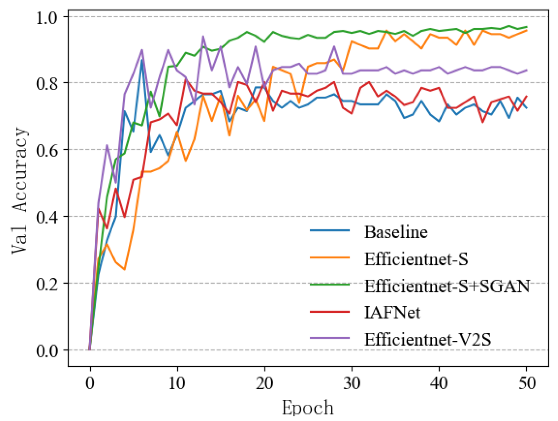
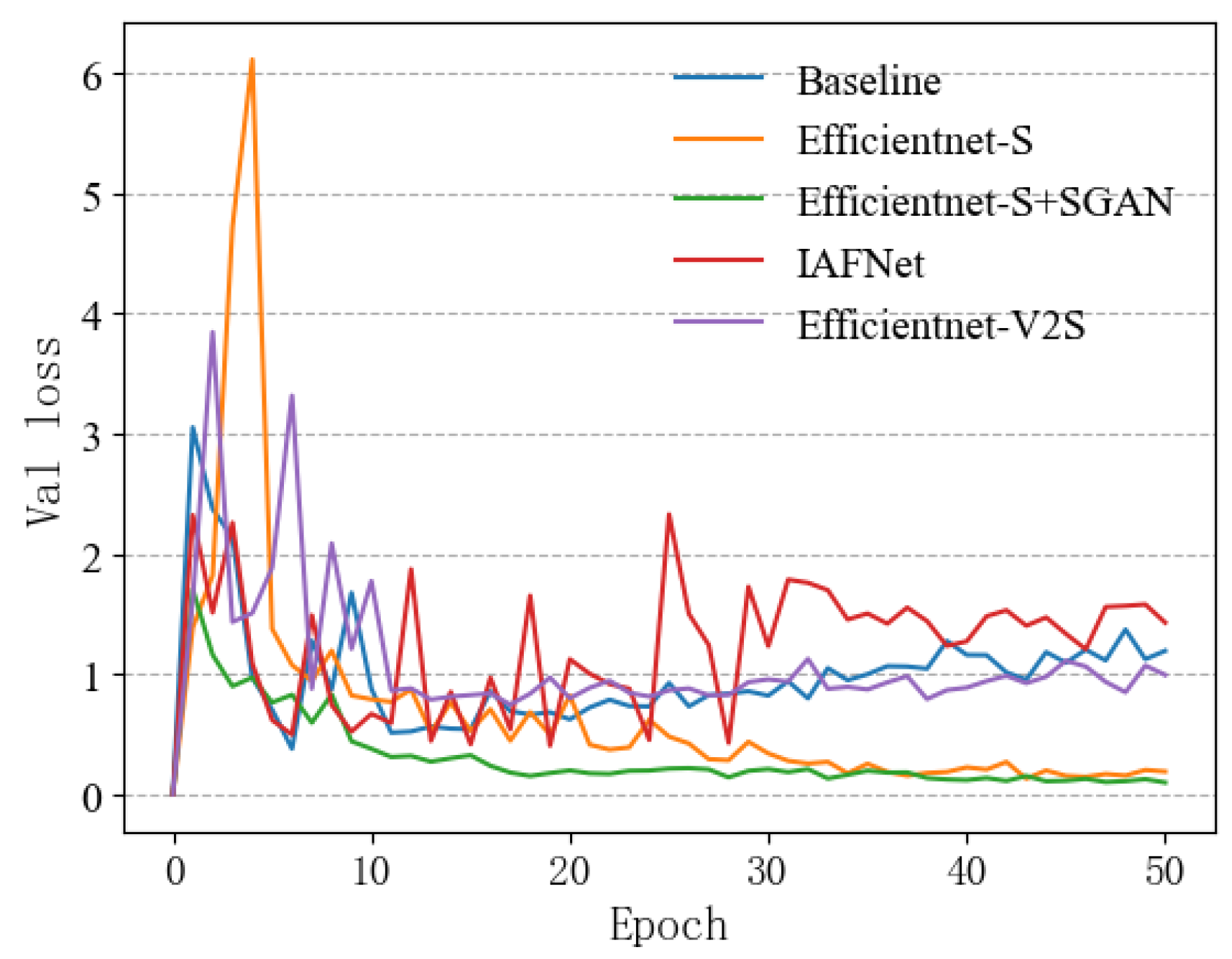
| Experiment Serial Number | Network Model | Test Set Accuracy (%) | Training Time (s) |
|---|---|---|---|
| 1 | Baseline | 78.8 | 223.5 |
| 2 | Efficientnet-S | 90.0 | 546.8 |
| 3 | Efficientnet-S+SGAN | 92.5 | 1203.6 |
| 4 | IAFNet | 73.8 | 411.2 |
| 5 | Efficientnet-V2S | 82.5 | 1108.7 |
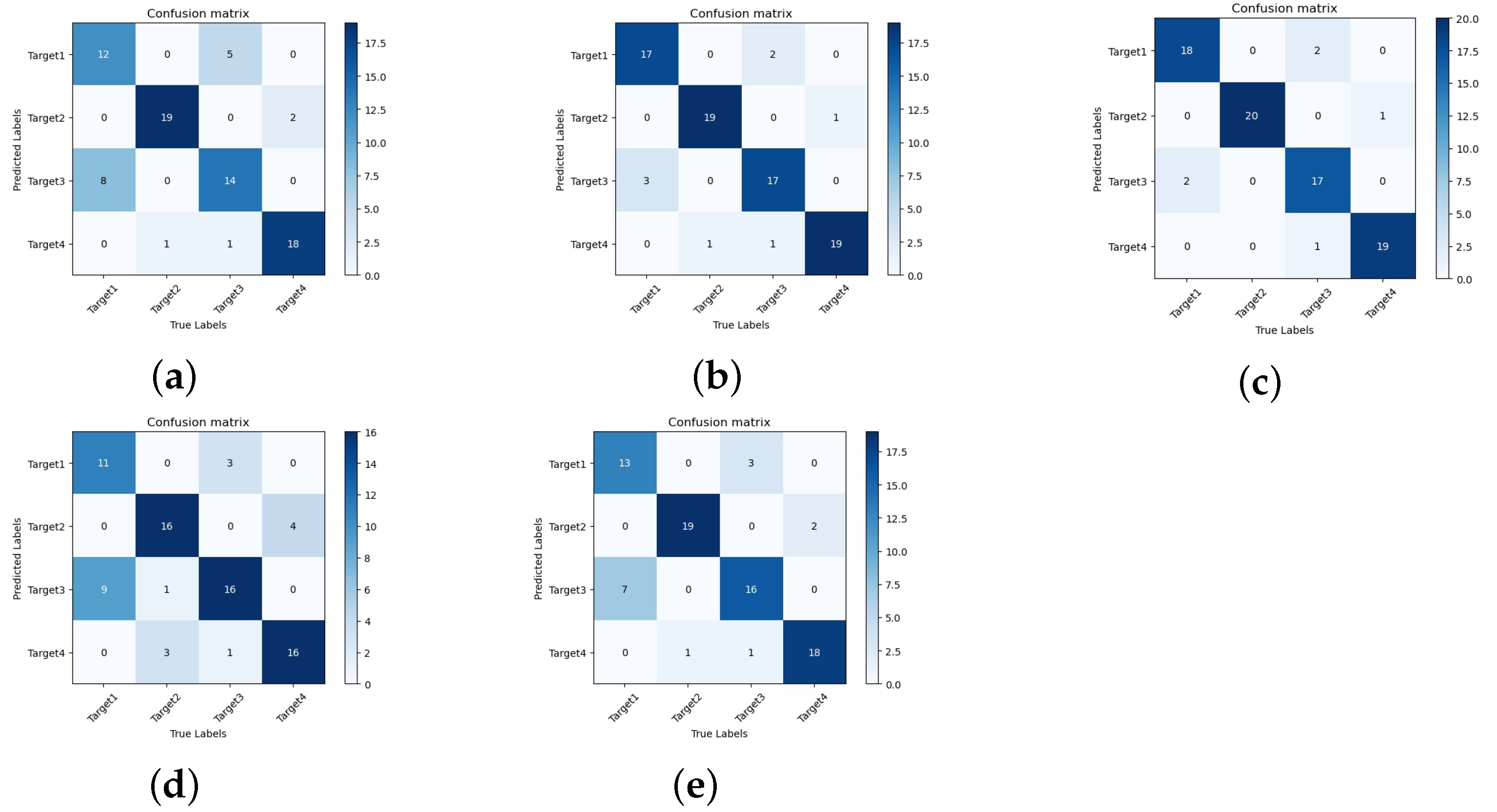
| Experiment Serial Number | Network Model | Average Precision (%) | Average Recall (%) | Average F1Score |
|---|---|---|---|---|
| 1 | Baseline | 78.68 | 78.75 | 0.7871 |
| 2 | Efficientnet-S | 90.00 | 90.00 | 0.9000 |
| 3 | Eff-S+SGAN | 92.43 | 92.50 | 0.9246 |
| 4 | IAFNet | 75.03 | 73.75 | 0.7438 |
| 5 | Efficientnet-V2S | 82.83 | 82.50 | 0.8266 |
Publisher’s Note: MDPI stays neutral with regard to jurisdictional claims in published maps and institutional affiliations. |
© 2022 by the authors. Licensee MDPI, Basel, Switzerland. This article is an open access article distributed under the terms and conditions of the Creative Commons Attribution (CC BY) license (https://creativecommons.org/licenses/by/4.0/).
Share and Cite
Chen, Y.; Liang, H.; Pang, S. Study on Small Samples Active Sonar Target Recognition Based on Deep Learning. J. Mar. Sci. Eng. 2022, 10, 1144. https://doi.org/10.3390/jmse10081144
Chen Y, Liang H, Pang S. Study on Small Samples Active Sonar Target Recognition Based on Deep Learning. Journal of Marine Science and Engineering. 2022; 10(8):1144. https://doi.org/10.3390/jmse10081144
Chicago/Turabian StyleChen, Yule, Hong Liang, and Shuo Pang. 2022. "Study on Small Samples Active Sonar Target Recognition Based on Deep Learning" Journal of Marine Science and Engineering 10, no. 8: 1144. https://doi.org/10.3390/jmse10081144
APA StyleChen, Y., Liang, H., & Pang, S. (2022). Study on Small Samples Active Sonar Target Recognition Based on Deep Learning. Journal of Marine Science and Engineering, 10(8), 1144. https://doi.org/10.3390/jmse10081144