Abstract
To comprehensively explore the characteristics of global SST anomalies, a novel time–frequency combination method, based on the COBE data and NCEP/NCAR reanalysis products in the past 100 years, was developed. From the view of the time domain, the global SST generally showed an upward trend from 1920 to 2019, the upward trend was significant after 1988, and the growth mutation occurred in 1930, according to the Mann–Kendall (MK) mutation test. Moreover, we extracted spatiotemporal modes of SST anomalies’ variability by empirical orthogonal function (EOF) analysis and obtained global spatial EOFs that closely correspond to regionally defined climate modes. Our results demonstrated that El Niño–Southern Oscillation (ENSO) is the typical character for the first mode of SST anomaly EOF, and Atlantic multidecadal oscillation (AMO) for the second. From the view of the frequency domain, our data suggested that there is a multi-period nesting phenomenon in global SST variations, in which the first main cycle with the most obvious oscillation was a 30-year cycle and changed in 20-year cycles, and the second cycle was a 15-year cycle and changed in 10-year cycles through wavelet analysis. As for the perspective of time–frequency characteristics, the dominant period of ENSO in the first mode of EOF is 4 years, obtained through filtering and cross wavelet transform. In addition, SST anomalies will maintain an upward trend for the next 60 months, according to the seasonal autoregressive integrated moving average (SARIMA) model, which has the potential value for predicting ENSO.
1. Introduction
The sea surface temperature (SST) and its anomalous variations are frequently utilized as the basis for the research of the El Niño or La Niña phenomena [1]. La Niña is the climatic phenomenon of abnormally decreasing SST in the East Central Pacific, while El Niño is the climatic phenomenon of abnormally increasing SST in the tropical Pacific Ocean [2,3]. Because of the greenhouse effect, the global climate has produced a major rise in both surface and ocean temperatures in recent years. In order to predict the El Niño or La Niña event, more research on the law of global SST changes is essential [4].
Because of the importance of SST, it is being studied by an increasing number of scholars, both at home and abroad. As an example, Zhang Z et al. [5] used the Optimum Interpolation Sea Surface Temperature provided by the National Oceanic and Atmospheric Administration of the United States to develop a model for SST prediction based on the gated recurrent unit algorithm, which they found to be more stable and accurate than the long short-term memory neural network model. Alekseev, GV et al. [6] used the monthly average data of Atlantic SST, provided by the Hadley SST Center, to investigate the relationship between the SST at low latitudes in the North Atlantic and the extent of Arctic sea ice through multivariate cross-correlation analysis, and proposed the formation mechanism of the long-range influence of low-latitude SST anomalies on the Arctic Ocean sea ice anomalies. He WB et al. [7] studied the contribution of SST anomalies in the tropical North Atlantic and equatorial Atlantic to El Niño–Southern Oscillation using the fifth generation European Centre for Medium-Range Weather Forecasts atmospheric reanalysis data and Hadley SST data. They observed that the SST anomalies in the equatorial Atlantic in summer was the result of the interaction between the tropical Atlantic and the Pacific Ocean, and that the equatorial Atlantic can affect the equatorial Pacific by transmitting or amplifying the SST anomalies in the tropical North Atlantic. Wu RG et al. [8] examined the contribution of El Niño–Southern Oscillation and the East Asian winter monsoon to the SST anomalies in the South China Sea during the two periods, and found that the SST anomalies in the first period were related to the East Asian winter monsoon, while the SST anomalies in the second period were mainly due to El Niño–Southern Oscillation. Through the heat budget analysis, it was concluded that the horizontal convection changes in shortwave radiation and surface latent heat flux were the explanations for the correlation between East Asian winter monsoon and SST anomalies. Ferster B S et al. [9] studied ENSO-Southern Ocean teleconnections based on the Optimal Interpolated Sea Surface Temperature’s version product and found that the positive patterns of Antarctic Oscillation and Southern Oscillation could drive SST cooling in high latitudes of the Southern Ocean and a warming trend within the Southern Hemisphere subtropical and mid-latitude regions. Gomez AM et al. [10] compared the CoralTemp of NOAA’s Coral Reef Watch, the UK Meteorological Office’s Operational SST and Sea Ice Analysis, and the global 1 km-SST of NASA’s Jet Propulsion Laboratory with in-situ observation data, and discovered that there is a significant positive correlation between the three satellite data and the in-situ observation data, but the SST of the satellite is about 1 degree lower than that of the in-situ observation. Duan XY et al. [11] discovered that under the El Niño phenomenon, the local SST rise was around 0.4 Celsius by using the Extended Reconstructed Sea Surface Temperature data and reanalysis data from 1979 to 2016. Messie M and Chavez F [12] conducted an empirical orthogonal function analysis of global SST anomalies using 100-year SST data provided by the Hadley SST Center, and discovered that the first six spatial modes correspond to the following six regional climate phenomena: El Niño–Southern Oscillation, the Pacific Decadal Oscillation, Atlantic Multidecadal Oscillation, North Pacific Gyre Oscillation, El Niño Modoki and the Atlantic El Niño. Wang X et al. [13] applied nonlinear Laplacian spectral analysis to study variability in the Southern Ocean associated with the Antarctic circumpolar wave, and discovered that the wavenumber-2 ACW mode with a 4-year period family recovered from Antarctic SST data correlates strongly with the ENSO mode family recovered from Indo-Pacific SST. Reynolds R W and Smith T M [14] compared and analyzed the global monthly SST using real-time lime in-situ (ship and buoy) and satellite data. During the 24 months from January 1985 to December 1986, the average monthly error of the SST data from the quality control drifting buoy was 0.78 Celsius, and the average absolute value of the monthly variation was 0.09 Celsius. Shirvani A et al. [15] established an autoregressive integrated moving average model to predict the SST of the Persian Gulf based on Extended Reconstructed Sea Surface Temperature data, provided by NOAA, in the tropical Indian Ocean region from 1950 to 2006.
Most scholars have focused their research on SST in specific regions, such as the Pacific Ocean, Atlantic Ocean or Indian Ocean, with less attention paid to the global SST. In addition, SST data are regularly updated as time passes, which makes it particularly vital to use the latest observational data to examine the changing laws of global SST. Taking this as the starting point, this paper uses the COBE-SST from 1920 to 2019 to examine the time–frequency characteristics of global SST anomalies. Through EOF analysis of 100-year SST anomalies, six modes are obtained, and the first three modes are focused on. Simultaneously, the relationship between wind and SST anomalies is preliminarily discussed, and the SARIMA model is utilized to forecast the range of global SST anomalies over the next 60 months.
2. Materials and Methods
2.1. Data Source and Processing
The monthly mean SST provided by Physical Sciences Laboratory (PSL) from 1920 to 2019 was adopted in this paper, the spatial resolution was 1 degree × 1 degree (latitude × longitude), the selected time range was from January 1920 to December 2019, and the length of the time series was 1200 months. COBE-SST is a composite SST series that integrated data from ships, buoys and satellites. Satellite observations are newly introduced for the purpose of reconstruction of SST variability over data-sparse regions. Moreover, uncertainty in areal means of the present and previous SST analyses is investigated using the theoretical analysis errors and estimated sampling errors. Thus, this data set has good superiority and reliability [16,17,18,19]. Southern Oscillation Index (SOI), Atlantic Multidecadal Oscillation (AMO) Index and Nino1 + 2 Index are all from the Climate Indices provided by PSL. The U-wind and V-wind data are NCAR/NCEP reanalysis products, and the time range is 1970–2019. The East Central Pacific region selected in this paper is (11° S~8° N, 172° W~102° W), the selected Indian Ocean region is (24° S~18° N, 55° E~90° E), the North Pacific region is selected as (22° N~29° N, 127° W~112° W), and the selected Atlantic region is (180°~40° E, 49° N~62° N). In this paper, the average value from 1920 to 2019 is regarded as the climatic average, and the process of subtracting this climatic average from the SST field to obtain the SST anomaly field is called anomaly processing.
2.2. Methods
2.2.1. Wavelet Analysis
The extended time series of global SST anomalies is non-stationary because it is easily influenced by other causes. As a result, time domain analysis cannot accurately determine the periodicity of time series. The study of non-stationary time series will be influenced by unpredictability and multi-time scale nesting. Wavelet analysis may clearly express the many periods buried in the time series and anticipate the short-term future trend from the standpoint of time–frequency combination [20,21]. Noise removal and filtering of SST time series, identification of periodic components, analysis of multi time scales, and other techniques are used to investigate it. In this study, the Morlet mother wavelet is utilized, and the formula is Equation (1).
In Equation (1), ω is the dimensionless frequency. When it is set as a constant 6 in this paper, the wavelet scale and Fourier period are roughly equal; the continuous wavelet change expression is shown by Equation (2).
In Equation (2), f(t) is the given signal, is the complex conjugate function of , a is the period length, b is the translation time, a, b ∈ R, a ≠ 0; the wavelet variance expression is shown by Equation (3).
2.2.2. Empirical Orthogonal Function
Principal component (PC) analysis is employed in the empirical orthogonal function (EOF) analysis of this research to decompose the time-varying SST field into spatial function and time coefficient parts [22,23]. The spatial function part is distinguished by the fact that it simply describes the regional distribution of the SST field, which does not change over time; the time coefficient is made up of a linear combination of SST [24,25]. One must select the appropriate spatial mode based on the principal component’s variance contribution rate, where the variance contribution rate necessitates the variable’s estimated value at the jth time of the ith grid point, which is stated as Equation (4).
In Equation (4), is the value of the ith lattice point of the kth eigenvector; is the value of the jth time in the kth time function. Then, the kth eigenvector and the ith lattice variance of the variable field of the time function are obtained, which are expressed as Equation (5).
In Equation (5), is the kth eigenvalue of the cross array of SST variable fields. Finally, the modal point variance contribution rate is obtained, which is expressed as Equation (6).
In Equation (6), is the variance of the ith lattice point. The variance contribution rate can express the main spatial regional variation information in the global SST mode.
2.2.3. Mann–Kendall Mutation Test
The forward and backward dual SST time series are calculated in the MK mutation test, and the forward and reverse curves are presented on the same graph. UFk is a positive SST time series curve, and UBk is an opposite SST time series curve that reverses to UFk. If the value of UFk > 0, it indicates that the time series has an upward trend; if the value of UFk < 0, it indicates that the time series represents a downward trend. If the intersection of the two dual curves falls inside the significant test range, it means the SST series has no substantial change trend in both the forward and reverse directions, and there may be a mutation in the trend change at the intersection [26,27]. If the intersection is outside the significant test range, the upward or downward trend is significant, and the range beyond the significant test range is the time period in which the significant trend occurs [28].
2.2.4. SARIMA Model
Curve fitting and parameter estimates are used to create the mathematical model. By using a difference operation, the long-term SST anomalies series is turned into a stationary time series. One must check that the autocorrelation diagram and partial autocorrelation diagram yields the p, q, d, q, Q, P and s within the ideal level to create an SARIMA model that is both rational and optimal, and then test it. The construction of a model of SST anomalies can be used to predict El Niño and other phenomena [29]. Figure 1 depicts the SARIMA process schematic.
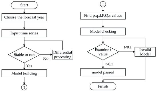
Figure 1.
SARIMA flow diagram.
3. Results
3.1. Temporal and Spatial Distribution of Global SST Anomalies
The global SST anomalies have removed the linear and seasonal trends from 1920 to 2019 in this part, and the variance distribution of SST anomalies is presented, as shown in Figure 2. The locations of SST anomalies may be shown to be predominantly concentrated in the East Central Pacific, the North Pacific, and some Atlantic regions, with the East Central Pacific being the birthplace of El Niño or La Niña.
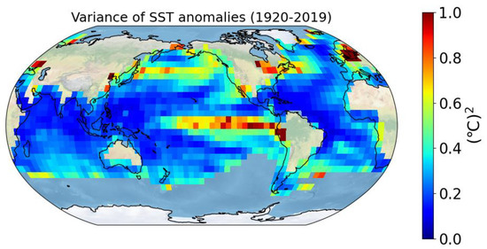
Figure 2.
Variance distribution of global SST anomalies from 1920 to 2019.
Further study on the spatial distribution of SST anomalies, the approximately 100-year period, which has been separated into the following nine stages: 1920–1930, 1931–1941, 1942–1952, 1953–1963, 1964–1974, 1975–1985, 1986–1996, 1997–2007 and 2008–2019, and the corresponding spatial distribution of global SST anomalies are shown in Figure 3. It can be observed that the anomalous value of global SST has risen steadily over the last 100 years, reaching a peak in the average region in the last 11 years. The first obvious anomalies developed in the North Pacific region between 1997 and 2007, with a mean value of almost 1.7 Celsius. In the past 30 years, the global SST anomalies changes have been more intense than the previous 70 years, and the overall upward trend in the past 100 years.
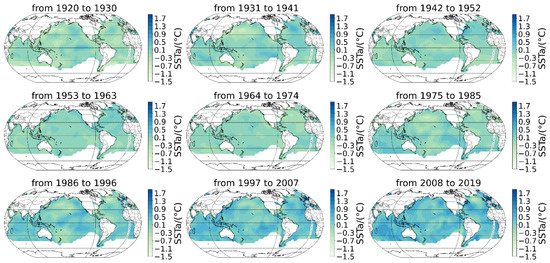
Figure 3.
Global distribution of SST anomalies with an interval of 11 years from 1920 to 2019.
3.2. SST Anomalies EOF
Through EOF analysis, the SST anomalies with seasonal and linear trends removed are converted into spatial modes of physical quantities and the corresponding temporal projections, and six SST anomalies modes are obtained. Table 1 shows the contribution rates of each mode. These six modes account for 43.48 percent of all SST anomalies. The magnitude of variance is used to represent the spatial distribution of global SST anomalies. In addition, the first mode has much more SST anomalies than the other five modes, with 20.83 percent.

Table 1.
The variance contribution and cumulative variance (unit: %) of the first 6 modes.
Figure 4a,b show the first mode and time coefficient of the global SST anomalies, respectively, with an explained variance of 20.83 percent. The time series of the first mode’s time coefficient and SOI index is shown in Figure 4c. After analyzing the time series, it was found that the correlation coefficient between SOI and the time coefficient of the first mode of SST anomalies reached 0.73, and it passed the 95% significance test. Furthermore, the first mode in Figure 4a depicts anomalies in the East Central Pacific, Indian Ocean, and North Pacific areas, which are quite similar to the ENSO mode. As a result, the ENSO mode is identified to be the first mode of SST anomalies. Combined with the time coefficient shown in Figure 4b, from 1920 to 2020, it mainly experienced “alternation of positive and negative-negative-positive-positive and negative”. Furthermore, the years with larger positive values were 1926, 1931, 1940–1942, 1972, 1982, 1987, 1998 and 2016; these years happen to be El Niño years. The years with larger negative values are 1924, 1942, 1950, 1956, 1971, 1973, 1975, 1988, 2000, 2008, 2010; these years are La Niña years.
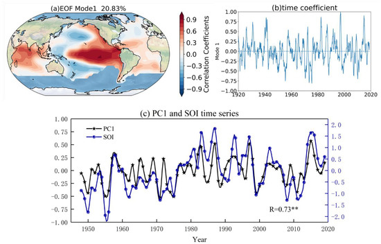
Figure 4.
The EOF of global SST anomalies. (a) The first mode, (b) time coefficient of the first mode, (c) the first mode’s time coefficient and SOI index, where the black line represents the time coefficient, the blue line represents the SOI index, ** represents the correlation coefficient R passed the 95% reliability test.
Figure 5a,b show the second mode and time coefficient of the global SST anomalies, respectively, with an explained variance of 6.32 percent. The time series of the second mode’s time coefficient and AMO index is shown in Figure 5c. After analyzing the time series, we found that the correlation coefficient between the AMO index and the second mode’s time coefficient of SST anomalies reached 0.85, and it passed the 95 percent significance test. Furthermore, the second mode in Figure 5a exhibits continuous anomalies across the Atlantic region and the second mode of SST anomalies is judged to be the AMO mode. From 1920 to 2020, it generally followed a “positive–negative–positive” trend, as illustrated by the time coefficient in Figure 5b.
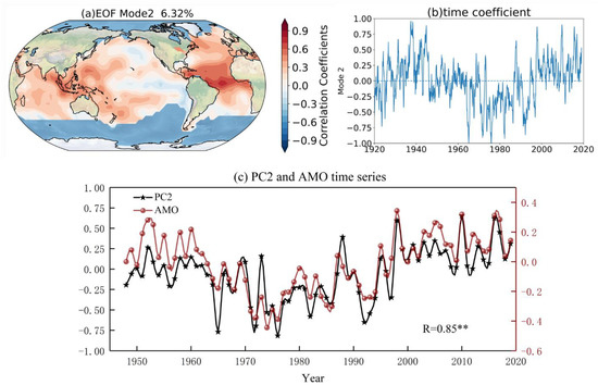
Figure 5.
The EOF of global SST anomalies. (a) The second mode, (b) time coefficient of the second mode, (c) the second mode’s time coefficient and AMO index, where the black line represents the time coefficient, the claret line represents the AMO index, ** represents the correlation coefficient R passed the 95% reliability test.
With an explained variance of 5.20 percent, Figure 6a,b depict the third mode and time coefficient of the global SST anomalies, respectively. The time series of the third mode’s time coefficient and Nino1 + 2 Index is shown in Figure 6c. The correlation coefficient between the Nino1 + 2 Index and the time coefficient of the third mode of SST anomalies reached 0.53 after analyzing the time series, but it failed to pass the significance test. Simultaneously, the spatial field distribution of the third mode in Figure 6a indicates that the third mode of the global SST anomalies may be the Pacific Decadal Oscillation (PDO) mode. As shown by the time coefficient in Figure 6b, it was always in shock from 1920 to 2020.
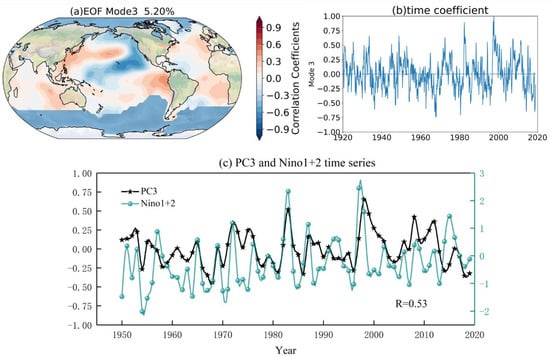
Figure 6.
The EOF of global SST anomalies. (a) The third mode, (b) time coefficient of the third mode, (c) the third mode’s time coefficient and Nino1 + 2 Index, where the black line represents the time coefficient and the sky blue line represents the AMO index.
3.3. Time Variation in SST Anomalies
Figure 7a depicts the global SST time series change during the last 100 years. It can be observed that the global SST generally shows an upward trend. The global SST has been rising since 1990, and after 2016, it is more than 0.5 Celsius higher than the perennial average, indicating that an El Niño event occurred in 2016. According to the calculations, the global SST is rising at a rate of 0.0069 Celsius. The annual SST change trend in the middle and eastern Pacific, the Indian Ocean, and the North Pacific is depicted in Figure 7b. It can be observed that the annual change trend between the central and eastern Pacific and the Indian Ocean is similar, while the annual change trend of SST in the North Pacific is the opposite. From July to September, the average SST in the East Central Pacific is at its highest, while the SST in the North Pacific is at its lowest. The mean SST in the East Central Pacific and Indian Ocean is generally steady between 26 and 28 Celsius, whereas the annual variance in the North Pacific varies substantially and remains between 18 and 23 Celsius.
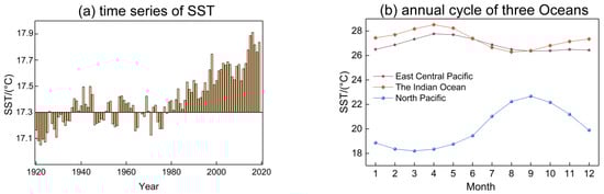
Figure 7.
Temporal variation in global SST from 1920 to 2019. (a) Time series of the SST, (b) annual cycle of the SST.
To take a closer look at the changing nodes of the SST, we divide the 1920–2019 period into two 50-year periods (1920–1969 and 1970–2019) for research. UFk is a positive SST time series curve, and Ubk is an opposite SST time series curve, which reverses to Ufk. If the value of Ufk > 0, it indicates that the SST has an upward trend; if the value of Ufk < 0, it indicates that the SST represents a downward trend. If the intersection of the two dual curves falls within the significant test range, it is considered that the time node corresponding to the intersection may have a trend mutation. If the intersection of the two dual curves does not fall within the significant test range, indicating that the upward or downward trend is significant, the time node that exceeds the significant test range is determined as the year with a significant trend. MK mutation tests are performed on the SST time series of the two time periods and the results are shown in Figure 8. It can be observed that the Ufk values are greater than 0 between 1923 and 1969, indicating that the SST shows an overall upward trend from 1923 to 1969, in which the mutation point occurs in 1930. Ufk values are greater than 0 from 1980 to 2019, but its mutation point occurs outside the significant test range. The intersection of Ufk and U95% occurs in 1988, indicating that the global SST has dramatically increased since 1988.
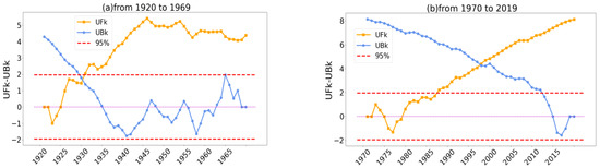
Figure 8.
Global SST MK test from 1920 to 2019. (a) From 1920 to1969, (b) from 1970 to 2019. The red dotted line contains 95% significant test range area.
3.4. Wavelet Analysis of Global SST Anomalies
The easiest technique to investigate the variation law of the global SST anomalies in the last 100 years is to look at its periodic fluctuation. The wavelet analysis of global SST anomalies with the long-term trends removed over the last 100 years is shown in Figure 9. We can notice the periodicity of the global SST anomalies and the abrupt change using a specific year as the boundary in the graphic. Simultaneously, we can discern a nested structure of numerous cycles, indicating that the cycle is not fixed in a certain time period. Figure 9a shows that there are cycles of 2–3 years, 7–8 years, 10–15 years, 20–25 years, 25–30 years and more than 30 years. The global SST anomalies will be in an abnormal rising period of 2–3-year, 15–20-year and more than 30-year cycles after 2020. The isoline of the global SST anomaly oscillation period over 30 years is not closed and is in an anomalous increasing period, as shown in Figure 6a, indicating that the global SST will continue to rise in this period for a long time.
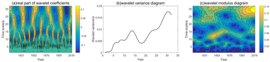
Figure 9.
Wavelet analysis of global SST anomalies. (a) Wavelet real part, (b) wavelet variance, (c) wavelet modulus.
Figure 9b shows that there are six distinct peaks, with time scales of 2 years, 6 years, 8 years, 15 years, 23 years, and 30 years. The wavelet variance peak corresponding to 30-year scale is the biggest among the different time scales, indicating that the 30-year cycle oscillation is the strongest in the global SST anomalies, which is the main cycle of SST anomalies. The wavelet variance for the 15-year scale is the second highest, indicating that 15 years is the second cycle of global SST anomalies, with 23-year, 8-year, 6-year, and 2-year scales representing the third, fourth, fifth, and sixth cycles, respectively.
The time distribution that corresponds to the modulus of the wavelet coefficient is shown in Figure 9c. The higher the modulus of the wavelet coefficient, the stronger the periodicity of the corresponding time scale. The modulus of the 30-year cycle is the largest in the process of the global SST anomalies during the past century, demonstrating most obviously its periodicity. The modulus of the 10–15-year period is the second, the modulus that corresponds to the 20–25-year period takes the third place, and the periodic change in the other time scales is not obvious.
One must select the first cycle and the second cycle that regulate the change in global SST anomalies, and build wavelet coefficient diagrams of corresponding time scales, as illustrated in Figure 10a,b. Different time scales correspond to different change cycles and high–low change characteristics, as may be observed from the overall pattern of changes. The variation cycle of the global SST anomalies that corresponds to the 30-year main cycle is about 20 years, with about 5 high-low variation phases in the past 100 years; the second cycle of 15 years corresponds to a 10-year cycle of global SST anomalies, with around 10 high–low variation phases.
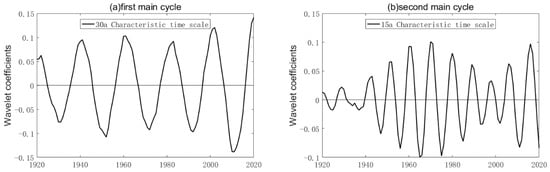
Figure 10.
Characteristic time scale variation in global SST anomalies. (a) First main cycle, (b) second main cycle.
To better study the interannual cycle of SST anomalies, we performed wavelet analysis on the 3–8-year band-pass filtered SST anomalies time series (Figure 11). The results show that the filtered time series has a very strong 3–4-year period and a weak 1-year period. As it is well known, ENSO has an interannual cycle of 2–8 years, which makes it hard not to assume that there is some connection between the two.
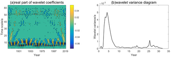
Figure 11.
Wavelet analysis of global SST anomalies with 3–8-year band-pass filtered. (a) Wavelet real part, (b) wavelet variance.
3.5. Influence of Wind Speed and Direction Characteristics on SST
The wind speed and direction on the sea surface can have a great impact on SST, and wind stress drives ocean circulation via frictional Ekman transport in the surface layer [30]. At first, we analyzed the wind field. Figure 12 shows that northeasterly winds prevail in spring and winter, while southwesterly winds prevail in summer and autumn in the North Indian Ocean. The reason for the former is the difference in thermal properties between land and sea (cold high pressure forms on the Asian continent in winter, low pressure forms on the ocean, the North Indian Ocean is at the southwest corner of the high pressure, and the wind blows from high pressure to low pressure). The reason for the latter is that the pressure and wind belt change with the season of the direct solar point. The direct solar point enters the Northern Hemisphere in summer. The southeast trade wind in the Southern Hemisphere moves northward across the equator and enters the Northern Hemisphere, and it is transformed into a southwesterly wind by the rightward geostrophic deflection force. Easterly winds prevail throughout the year in the central and eastern Pacific, with the strongest in summer, the second in autumn, the third in winter, and the weakest in spring. The reason for the year-round prevailing northwesterly winds in the North Pacific may be that the mid-latitude westerly winds in the Northern Hemisphere are influenced by the direction of their rotation (clockwise in the Northern Hemisphere) as they blow over the Hawaiian high, thereby changing from west winds to northwest winds (Figure 12).
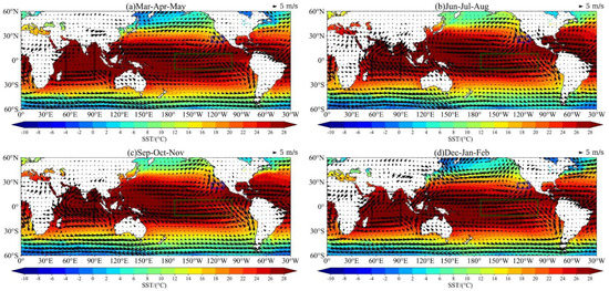
Figure 12.
Surface wind field and SST of the ocean. (a) Mar–Apr–May, (b) Jun–Jul–Aug, (c) Sep–Oct–Nov, (d) Dec–Jan–Feb. The arrow shows wind direction, the blue boxed area, red boxed area and green boxed area are the part of the North Pacific, Indian Ocean and central and eastern Pacific Ocean studied in this paper.
Then, we analyzed the connection between wind field and SST. The southeast monsoon powers the heat accumulation in the tropical southern Indian Ocean. The enhanced wind speed causes the cold water in the high latitudes of the North Pacific to accelerate to the northeast, resulting in a strong cold signal in the middle and high latitudes. The northeast trade winds between 0° and 18° N intensify and move slightly southward, which promote the accelerated westward transport of cold water at low latitudes in the southeastern North Pacific, resulting in a decrease in SST in the low latitude seas. In the 35–60° N region of the North Pacific, the wind speed changes only slightly, basically below 1 m/s, which is not enough to explain the dramatic decrease in SST in this region in Figure 12. It is speculated that it is mainly caused by atmospheric cooling. The presence of easterly winds causes a large amount of surface warm water to be blown to the equatorial western Pacific region, which means that the warm water in the equatorial eastern Pacific region is swept away, and the surface seawater in the eastern Pacific region is mainly supplemented by cold water below the sea surface. Therefore, the SST in the equatorial eastern Pacific is significantly lower than that in the western Pacific (La Niña). When the El Niño (La Niña) develops in the central and eastern Pacific Ocean, the tropical Indian Ocean’s SST in the following year tends to show consistent warming (colder) through the atmospheric bridge and the Indian Ocean through-flow [31,32,33].
3.6. Short-Term SARIMA Forecast
Stationary time series is a necessary condition for constructing the SRIMA (p, d, q) (P, D, Q, s) model. In Section 3.3 of this paper, we stated that the SST anomalies time series is a non-stationary series, which has a clear upward trend. Thus, we obtain a stationary time series from the series of SST anomalies using first-order differences and seasonal difference. In fact, this can be observed from Figure 13a where there is a clear trend, so the mean is not constant and the variance across the series is relatively unstable. Before modeling, we first processed the seasonality of SST anomalies by seasonal difference. The result after seasonal difference is shown in Figure 13b. It can be observed that the p-value has dropped from around 0.5 to 0, and the values of the autocorrelation function (ACF) and the partial autocorrelation function (PACF) are mostly concentrated in the shaded area. It indicates that the seasonality of SST anomalies must be removed. Secondly, we also need to remove the long-term trends of SST anomalies, and the result after processing by first-order difference is shown in Figure 13c. It can be observed that the p-value still remains at 0, and the values of ACF and PACF are almost all within the shaded area. This indicates that the long-term trend of SST anomalies is also removed. Finally, the optimal result obtained by combining the seasonal difference and the first-order difference is shown in Figure 13d.
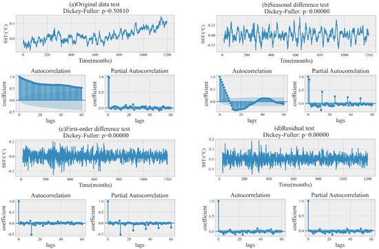
Figure 13.
Construction process of SARIMA model. (a) Original data test, (b) seasonal difference test, (c) first-order difference test, (d) residual test.
The p in the SARIMA model represents the maximum lag value of the model, which can be found in PACF. The maximum lag that can be obtained in the PACF figure of the optimal result is 6, indicating that the p is most likely to be 6. The q is the same as p, but it is obtained from the ACF figure. In addition, the maximum lag in the ACF figure is 6, which means that the q may be 6. The d and D are set to 1 because we are using first-order difference and seasonal difference. The s is the seasonal cycle and is set to 12 in this paper. The P is the order of the seasonal component of the autoregressive model, which is a multiple of s. It can be observed from the PACF that the 24th point lags significantly, indicating that the P is 2. The Q is also 2, but from the ACF. In summary, the optimal model constructed in this paper is SARIMA (6, 1, 6) (2, 1, 2, 12).
After constructing the optimal SARIMA model, one can use this model to forecast the global SST anomalies for the next 60 months. In this paper, the model represents the prediction of SST anomalies in the past 100 years under the SARIMA model (1200 months as a comparison verification, 60 months as a prediction), and represents the time series of global SST anomalies in the past 1200 months. By observing Figure 14, it can be observed that the actual value of the first 1200 months is almost the same as the model value, and the accuracy is very high. This shows that the SARIMA model we constructed is credible and valuable. In addition, we predict that the global SST anomalies will still be on an upward trend in the next 60 months, which is a phenomenon worth pondering.
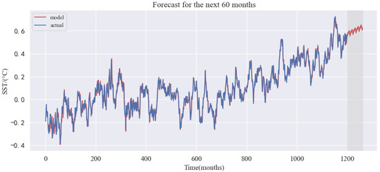
Figure 14.
Prediction of global SST anomalies in the next 60 months.
4. Discussion
In this paper, it is discovered that the East Central Pacific, the North Pacific, and some parts of the Atlantic have experienced large fluctuations in SST anomalies over the past century. Chen SF et al. [34] investigate the relationship between North Atlantic SST and North Atlantic Oscillation, Wu RG et al. [35] investigate the relationship between tropical Pacific SST and precipitation in the Indochina Peninsula, Wu MM and Wang L [36] analyze the relationship between the summer nino3.4 index and North Pacific summer monsoon index and Yook S et al. [37] reveal two atmospheric variability models of winter variation in SST in the mid latitude of the North Pacific. Almost of their research focused on the North Pacific, Indian Ocean or Atlantic Ocean, which shows that these seas are complex with regard to climate change and are the focus areas of research. While this paper mainly studies SST anomalies on a global scale, the conclusions drawn are close to the results of these researchers. According to the EOF of SST anomalies, the first mode of SST anomalies is ENSO, and the second mode is AMO. This result is consistent with the 100-year EOF analysis of global SST anomalies by Messié M et al. [12], which discovered that the first six modes correspond to the following six regional climate phenomena: El Niño–Southern Oscillation, the Pacific Decadal Oscillation, Atlantic Multidecadal Oscillation, North Pacific Gyre Oscillation, El Niño Modoki, and the Atlantic El Niño. However, Chen X et al. [38] performed the conventional EOF decomposition of the SST, discovering that the first mode is dominated by the global warming trend, the second contains ENSO in the tropical Pacific and is commonly referred to as being “ENSO-like” and the third mode has a spatial pattern with warming in the North Atlantic and cooling in the South Atlantic. In fact, in the EOF decomposition of SST anomalies in this paper, the long-term and seasonal trend of the data have been removed, so there is no global warming trend in the first mode. When the SARIMA model is used to forecast the SST anomalies in the following 60 months, the abnormal fluctuation is estimated to be around 0.5 Celsius and will continue to rise, which is comparable to the result of Shirvani A et al. [15], who used the ARIMA model to predict SST in the Persian Gulf.
SST anomalies after continuous wavelet transform show the oscillation cycles of 2 years, 6 years, 8 years, and 15 years; this result is compatible with the findings of Silva C B et al. [39]. They found that global sea surface temperature exists in the 1–12-month and 1–2-, 2–4-, 4–8-, and 8–12-year oscillation cycles. The 2–8-year cycle is easily associated with ENSO [40], and the first mode after EOF decomposition of the SST anomalies in this paper is similar to ENSO. Thus, we perform wavelet analysis on the 3–10-year band-pass filtered PC1 coefficient and Figure 15 shows that the 3–10-year band-pass filtered PC1 coefficient exhibits a strong 4-year period. The following Figure 16 also verifies the existence of a 4-year resonance period between the SOI and SST anomalies.
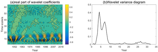
Figure 15.
Wavelet analysis of the PC1 coefficient with 3–10-year band-pass filtered. (a) Wavelet real part, (b) wavelet variance.
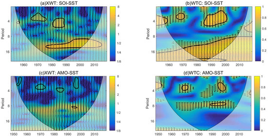
Figure 16.
Cross wavelet analysis of SOI, AOM and SST anomalies. (a,b) SOI and SST anomalies, (c,d) AOM and SST anomalies. The area enclosed by the black solid line is the area that passes the 95% test. The direction of the arrow indicates the correlation between the two. The arrow to the right indicates a positive correlation, the arrow to the left indicates a negative correlation, the upwards arrow indicates the lead quarter cycle, and the downwards arrow indicates a quarter cycle behind.
According to the characterization of ENSO and AMO as the first two modes of EOF decomposition of SST anomalies, the cross wavelet transform of SOI and AMO with SST anomalies was carried out respectively, as shown in the Figure 16. The cross wavelet transform can not only analyze the relationship between the two parameters, but also reflect their phase structure and detailed characteristics in the time domain and frequency domain. The cross wavelet energy spectrum in Figure 16a showed that there are three resonance periods for SOI and SST anomalies that pass the 95 percent test, which were the 3-year period (1963 to 1975), 4–5-year period (1981 to 1989) and 10–14-year period (1976 to 2005); the correlation between the two changed abruptly around 1994, from a negative correlation before 1976 to a positive correlation. These results are compatible with the work of Venegas S A [41] and Cerrone D et al. [42]. The former found a 5-year period signal in the local fractional variance spectrum for the SST anomalies, arguing that this signal was the tropical ENSO response over the Southern Oscillation; the latter performed a study on the real part of the first three complex empirical orthogonal functions (CEOFs) for the SST anomalies using spectral analysis, arguing that the dominant periods of the CEOFSST1, CEOFSST2 and CEOFSST3 were the 4.7-year, 4.9-year and 4.9-year periods. Contrary to their conclusion, we considered that in addition to the 4-year response cycle, there might be a 10–14-year response decadal cycle. Figure 16b reveals that the resonance periods of the 3-year period, 4–5-year period, and 10–14-year period all pass the significant test, especially the 10–14-year period, which shows a large-scale significant positive correlation. Combining this with the spatial distribution of the SST anomalies in Section 3.1, it is discovered that the SST anomalies fluctuated more severely after 1970, indicating that ENSO may have been the primary reason for the SST anomalies from 1970 to 2008. In addition, whether it is the filtered SST anomalies or the PC1 coefficient, or the resonance period of SOI and SST anomalies, there is an extremely obvious 4-year period. Therefore, the 4-year cycle may be the dominant cycle for SST anomalies in response to ENSO. With regard to AMO, it warrants further investigation in future work.
5. Conclusions
The time–frequency characteristics of global SST anomalies were investigated using COBE-SST data from January 1920 to December 2019. Following the preliminary investigation and discussion, the following conclusions were reached:
- (1)
- By calculating the regional variance in SST anomalies in the past 100 years, the regions with larger anomalous fluctuations appear in the East Central Pacific, North Pacific and parts of the Atlantic.
- (2)
- The first EOF mode of SST is characterized as ENSO, and the El Niño/La Niña years are verified by the positive and negative values of the corresponding time coefficients; the second mode of EOF of SST is characterized as AMO.
- (3)
- The global SST generally showed an upward trend from 1920 to 2019, the upward trend was significant after 1987, and growth mutation occurred in 1930.
- (4)
- Global SST anomalies have multi-scale nested cycles of 2–3 years, 7–8 years, 10–15 years, 20–25 years, 25–30 years, and 30 years, as shown by wavelet analysis.
- (5)
- The SARIMA model predicts that SST anomalies will still be on an upward trend in the next 60 months.
With a deepened understanding of the ocean–atmosphere interaction and its variability, the variable characteristics of SST anomalies have received increased attention. Moreover, the examination of the fluctuation characteristics of SST anomalies can be utilized to forecast the El Niño or La Niña events. In this paper, wavelet analysis is utilized to examine the frequency domain change cycle of global SST anomalies. Simultaneously, the SARIMA model is utilized to forecast SST anomalies for the following 60 months. Meanwhile, the reasons for global SST anomalies are preliminarily discussed, and an in-depth investigation is required for the root causes.
Author Contributions
C.T.: Methodology, Software, Visualization and Writing—original draft. D.H.: Methodology, Writing—original draft, Writing—review and editing. Y.W.: Funding Acquisition and Validation. F.Z.: Investigation and Validation. X.W.: Investigation and Resources. X.T.: Investigation and Validation. All authors have read and agreed to the published version of the manuscript.
Funding
This study is supported by the Scientific Research Start-up Fund for High-Level Introduced Talents of Anhui University of Science and Technology (Grant number No. 13190007), the University Natural Science Research Project of Anhui Province of China (Grant number No. KJ2019A0103; KJ2021A0447), the Specialized Research Fund for State Key Laboratories (Grant number No. 201909) and National Key Research and Development Program (Grant number No. 2017YFD0700501).
Institutional Review Board Statement
Not applicable.
Informed Consent Statement
Not applicable.
Data Availability Statement
The U-wind and V-wind Reanalysis products were downloaded from https://psl.noaa.gov/data/gridded/data.ncep.reanalysis.html (Recently accessed date: 13 June 2022). The COBE-SST were downloaded from http://ds.data.jma.go.jp/tcc/tcc/products/elnino/cobesst/cobe-sst.html (Recently accessed date: 16 June 2022). The SOI Index and AOM Index were downloaded from https://psl.noaa.gov/data/climateindices/list/ (Recently accessed date: 27 May 2022).
Acknowledgments
We would like to thank PSL and the Japanese Oceanographic Data Center for providing the necessary datasets used in this study.
Conflicts of Interest
The authors declare that there are no conflict of interest regarding the publication of this paper.
References
- Feng, L.C.; Liu, F.; Zhang, R.H.; Han, X.; Yu, B.; Gao, C. On The second-year warming in late 2019 over the Tropical Pacific and its attribution to an Indian Ocean Dipole event. Adv. Atmos. Sci. 2021, 38, 2153–2166. [Google Scholar] [CrossRef]
- van Loon, H.; Meehl, G.A. The response in the Pacific to the sun’s decadal peaks and contrasts to cold events in the Southern Oscillation. J. Atmos. Sol.-Terr. Phys. 2008, 70, 1046–1055. [Google Scholar] [CrossRef]
- Meehl, G.A.; Arblaster, J.M.; Matthes, K.; Sassi, F.; van Loon, H. Amplifying the Pacific climate system response to a small 11-year solar cycle forcing. Science 2009, 325, 1114–1118. [Google Scholar] [CrossRef] [Green Version]
- Zhou, Q.; Duan, W.; Hu, J. Exploring sensitive area in the tropical Indian Ocean for El Niño prediction: Implication for targeted observation. J. Oceanol. Limnol. 2020, 38, 1602–1615. [Google Scholar] [CrossRef]
- Zhang, Z.; Pan, X.L.; Jiang, T.; Sui, B.K.; Liu, C.X.; Sun, W.F. Monthly and quarterly sea surface temperature prediction based on gated recurrent unit neural network. J. Mar. Sci. Eng. 2020, 8, 249. [Google Scholar] [CrossRef] [Green Version]
- Alekseev, G.V.; Kuzmina, S.I.; Glok, N.I.; Vyazilova, A.E.; Ivanov, N.E.; Smirnov, A.V. Influence of Atlantic on the warming and reduction of sea ice in the Arctic. Ice Snow 2017, 57, 381–390. [Google Scholar] [CrossRef] [Green Version]
- He, W.B.; Ma, J. Interaction between the Tropical Atlantic and Pacific Oceans on an Interannual Time Scale. Atmosphere-Ocean 2021, 59, 285–298. [Google Scholar] [CrossRef]
- Wu, R.G.; Chen, W.; Wang, G.H.; Hu, K.M. Relative contribution of ENSO and East Asian winter monsoon to the South China Sea SST anomalies during ENSO decaying years. J. Geophys. Res. Atmos. 2014, 119, 5046–5064. [Google Scholar] [CrossRef]
- Ferster, B.S.; Subrahmanyam, B.; Macdonald, A.M. Confirmation of ENSO-Southern Ocean teleconnections using satellite-derived SST. Remote Sens. 2018, 10, 331. [Google Scholar] [CrossRef] [Green Version]
- Gomez, A.M.; McDonald, K.C.; Shein, K.; DeVries, S.; Armstrong, R.A.; Hernandez, W.J.; Carlo, M. Comparison of satellite-based sea surface temperature to in situ observations surrounding coral reefs in La Parguera, Puerto Rico. J. Mar. Sci. Eng. 2020, 8, 453. [Google Scholar] [CrossRef]
- Duan, X.Y.; Xue, F.; Zheng, F. Sea surface temperature anomalies in the tropical North Atlantic during El Nino decaying year. Atmos. Ocean. Sci. Lett. 2021, 14, 16–21. [Google Scholar] [CrossRef]
- Messie, M.; Chavez, F. Global modes of sea surface temperature variability in relation to regional climate indices. J. Clim. 2011, 24, 4313–4330. [Google Scholar] [CrossRef]
- Wang, X.; Giannakis, D.; Slawinska, J. The Antarctic circumpolar wave and its seasonality: Intrinsic travelling modes and El Niño–Southern Oscillation teleconnections. Int. J. Climatol. 2019, 39, 1026–1040. [Google Scholar] [CrossRef]
- Reynolds, R.W.; Smith, T.M. Improved global sea surface temperature analyses using optimum interpolation. J. Clim. 1994, 7, 929–948. [Google Scholar] [CrossRef] [Green Version]
- Shirvani, A.; Nazemosadat, S.M.J.; Kahya, E. Analyses of the persian gulf sea surface temperature: Prediction and detection of climate change signals. Arab. J. Geosci. 2015, 8, 2121–2130. [Google Scholar] [CrossRef]
- Hausfather, Z.; Cowtan, K.; Clarke, D.C.; Jacobs, P.; Richardson, M.; Rohde, R. Assessing recent warming using instrumentally homogeneous sea surface temperature records. Sci. Adv. 2017, 3, e1601207. [Google Scholar] [CrossRef] [PubMed] [Green Version]
- Mather, J.C. Nobel lecture: From the big bang to the Nobel prize and beyond. Rev. Mod. Phys. 2007, 79, 1331. [Google Scholar] [CrossRef] [Green Version]
- Liu, Y.; Zhang, Y.; Cai, J.; Tsou, J.Y. Analyzing the Effects of Sea Surface Temperature (SST) on Soil Moisture (SM) in Coastal Areas of Eastern China. Remote Sens. 2020, 12, 2216. [Google Scholar] [CrossRef]
- Huang, B.; Angel, W.; Boyer, T.; Cheng, L.; Chepurin, G.; Freeman, E.; Liu, Y.; Zhang, H. Evaluating SST analyses with independent ocean profile observations. J. Clim. 2018, 31, 5015–5030. [Google Scholar] [CrossRef]
- Kumar, S.; Tiwari, M.K.; Chatterjee, C.; Mishra, A. Reservoir inflow forecasting using ensemble models based on neural networks, wavelet analysis and bootstrap method. Water Resour. Manag. 2015, 29, 4863–4883. [Google Scholar] [CrossRef]
- Dai, X.G.; Chou, J.F. Wavelet analysis on the runoffs of the Changjiang River and the Huanghe River. Theor. Appl. Climatol. 1996, 55, 193–197. [Google Scholar] [CrossRef]
- Hatzaki, M.; Wu, R.G. The south-eastern Europe winter precipitation variability in relation to the North Atlantic SST. Atmos. Res. 2015, 152, 61–68. [Google Scholar] [CrossRef]
- Takahashi, K.; Montecinos, A.; Goubanova, K.; Dewitte, B. ENSO regimes: Reinterpreting the canonical and Modoki El Niño. Geophys. Res. Lett. 2011, 38, L10704. [Google Scholar] [CrossRef] [Green Version]
- Mohamed, B.; Nagy, H.; Ibrahim, O. Spatiotemporal Variability and Trends of Marine Heat Waves in the Red Sea over 38 Years. J. Mar. Sci. Eng. 2021, 9, 842. [Google Scholar] [CrossRef]
- Tung, K.K.; Chen, X.Y.; Zhou, J.S.; Li, K.F. Interdecadal variability in pan-Pacific and global SST, revisited. Clim. Dyn. 2018, 52, 2145–2157. [Google Scholar] [CrossRef] [Green Version]
- Bian, Y.K.; Yue, J.P.; Gao, W.; Li, Z.; Lu, D.K.; Xiang, Y.F.; Chen, J. Analysis of the spatiotemporal changes of ice sheet mass and driving factors in Greenland. Remote Sens. 2019, 11, 862. [Google Scholar] [CrossRef] [Green Version]
- Buric, D.; Lukovic, J.; Ducic, V.; Dragojlovic, J.; Doderovic, M. Recent trends in daily temperature extremes over southern Montenegro (1951–2010). Nat. Hazards Earth Syst. Sci. 2014, 14, 5181–5198. [Google Scholar] [CrossRef] [Green Version]
- Ahmedou, O.C.A.; Yasuda, H.; Wang, K.; Hattori, K. Characteristics of precipitation in northern Mauritania and its links with sea surface temperature. J. Arid Environ. 2008, 72, 2243–2250. [Google Scholar] [CrossRef]
- Georgakarakos, S.; Koutsoubas, D.; Valavanis, V. Time series analysis and forecasting techniques applied on loliginid and ommastrephid landings in Greek waters. Fish. Res. 2006, 78, 55–71. [Google Scholar] [CrossRef] [Green Version]
- Zhang, Y.; Xu, H.; Qiao, F.; Dong, C. Seasonal variation of the global mixed layer depth: Comparison between Argo data and FIO-ESM. Front. Earth Sci. 2018, 12, 24–36. [Google Scholar] [CrossRef]
- Klein, S.A.; Soden, B.J.; Lau, N.C. Remote sea surface temperature variations during ENSO: Evidence for a tropical atmospheric bridge. J. Clim. 1999, 12, 917–932. [Google Scholar] [CrossRef] [Green Version]
- Lau, N.C.; Nath, M.J. Impact of ENSO on the variability of the Asian–Australian monsoons as simulated in GCM experiments. J. Clim. 2000, 13, 4287–4309. [Google Scholar] [CrossRef] [Green Version]
- Meyers, G. Variation of Indonesian throughflow and the El Niño-southern oscillation. J. Geophys. Res. Ocean. 1996, 101, 12255–12263. [Google Scholar] [CrossRef]
- Chen, S.F.; Wu, R.G.; Chen, W. The changing relationship between interannual variations of the North Atlantic Oscillation and northern tropical Atlantic SST. J. Clim. 2015, 28, 485–504. [Google Scholar] [CrossRef]
- Wu, R.G.; Shi, Y.; Zhu, P.J.; Jia, X.J. An interdecadal change in August Indochina Peninsula precipitation-ENSO relationship around 1980. Clim. Dyn. 2022, 1–16. [Google Scholar] [CrossRef]
- Wu, M.M.; Wang, L. Enhanced correlation between ENSO and western North Pacific monsoon during boreal summer around the 1990s. Atmos. Ocean. Sci. Lett. 2019, 12, 376–384. [Google Scholar] [CrossRef]
- Yook, S.; Thompson, D.W.J.; Sun, L.T.; Patrizio, C. The Simulated Atmospheric Response to Western North Pacific Sea Surface Temperature Anomalies. J. Clim. 2022, 35, 3335–3352. [Google Scholar] [CrossRef]
- Chen, X.; Tung, K.K. Global-mean surface temperature variability: Space–time perspective from rotated EOFs. Clim. Dyn. 2018, 51, 1719–1732. [Google Scholar] [CrossRef] [Green Version]
- Silva, C.B.; Silva, S.M.E.; Krusche, N.; Ambrizzi, T.; Ferreira, N.D.; Dias, P.L.D. The analysis of global surface temperature wavelets from 1884 to 2014. Theor. Appl. Climatol. 2019, 136, 1435–1451. [Google Scholar] [CrossRef]
- Trenberth, K.E. Spatial and temporal variations of the Southern Oscillation. Q. J. R. Meteorol. Soc. 1976, 102, 639–653. [Google Scholar] [CrossRef]
- Venegas, S.A. The Antarctic Circumpolar Wave: A combination of two signals? J. Clim. 2003, 16, 2509–2525. [Google Scholar] [CrossRef]
- Cerrone, D.; Fusco, G.; Cotroneo, Y.; Simmonds, I.; Budillon, G. The antarctic circumpolar wave: Its presence and interdecadal changes during the last 142 years. J. Clim. 2017, 30, 6371–6389. [Google Scholar] [CrossRef]
Publisher’s Note: MDPI stays neutral with regard to jurisdictional claims in published maps and institutional affiliations. |
© 2022 by the authors. Licensee MDPI, Basel, Switzerland. This article is an open access article distributed under the terms and conditions of the Creative Commons Attribution (CC BY) license (https://creativecommons.org/licenses/by/4.0/).