Research on the Evaluation of Logistics Efficiency in Chinese Coastal Ports Based on the Four-Stage DEA Model

Abstract

In the context of economic globalization, coastal port logistics has gradually become a focus of economic development, and the proper management of coastal port logistics performance is the main way to realize the high-efficiency operation of coastal ports, drives the direct economic development of the hinterland, and enhances import and export trade market competitiveness. Accordingly, this study was aimed to measure port logistics efficiency and explore its path of improvement for China’s coastal ports during the 2014–2018 period with a four-stage DEA model, including a Tobit model. The results of this study show that most of the coastal ports in China have emphasized their size more than their planning. During the study period, improving road network construction and the economic level in hinterland port cities was conducive to improving port logistics efficiency, but tertiary industry investment and foreign trade levels were negatively correlated with coastal port logistics efficiency.

1. Introduction

In logistics systems, ports have a significant role in a country’s productivity and competitiveness [1,2]. Based on international trade, the cargo throughput of China’s coastal ports has increased year-by-year in recent decades. According to relevant data, the cargo throughput increased from 5483.58 million tons in 2010 to 9480.02 million tons in 2020 (a growth rate of 73%) and the container throughput increased from 146 million TEUs in 2010 to 260 million TEUs in 2020 (a growth rate of 78%), which shows that the economic status is gradually improving (data originated from China Port Yearbook 2011 on the official website of the Ministry of Transport).

In an environment of such rapid technological and economic development, coastal ports have not only gained more opportunities but also faced some confusion and challenges. A primary problem to be solved in the development of China’s coastal ports is the removal of the traditional development model in order to promote benign interactions between ports and foreign trade and to actively expand the service depth of the hinterland economy [3]. In this process, the transformation to multi-functional, standardized, and integrated intelligent ports can occur through the use of the location and environment of the ports.

The logistics performance of coastal ports will also have a significant impact on the development of hinterland cities. Obviously, in order to achieve improved coastal port logistics efficiency, ports need to seize the opportunity. Depending on a coastal port’s conditions, it must reasonably invest in new equipment and facilities, as well as adjust its development model to increase output. However, before that, we first need to understand the overall status of logistics efficiency in coastal ports and to explore the path for its improvement in China.

Therefore, in this study, the logistics efficiency of coastal ports was accurately and systematically evaluated. The results of this study can help us understand the clear market positioning of each port. Additionally, solving the logistics inefficiency issue of coastal ports will improve research about port efficiency. The main contributions of this study are as follows. First, the input redundancy of 20 coastal ports is explained by introducing four environment variables (road network construction, economic level, foreign trade level, and scale of service industry). Second, the strengths of each port in each region are presented through cluster analysis based on a logistics efficiency throughput matrix. Third, the degree and direction of the impact of various environmental factors on port logistics efficiency are analyzed in order to explore the path of improvement for China’s coastal ports. This study provides a practical basis for port authorities and operators, and it may provide useful information to other ports in the world.

The remainder of this paper is organized as follows: in Section 2, we review the related literature. In Section 3, we describe the theoretical model. In Section 4, we introduce the variables and descriptions. Section 5, we analyze the empirical results. In Section 6, we present some concluding remarks and suggestions.

2. Literature Review

The literature closely associated with our work can be classified into three main categorizes: efficiency analysis based on four-stage data envelopment analysis (DEA), logistics efficiency evaluation, and logistics efficiency based on DEA.

2.1. Efficiency Analysis Based on Four-Stage DEA

DEA is a widely used mathematical programming approach that has been long-regarded as the standard non-parametric tool for evaluating the relative efficiency of decision-making units (DMUs) in organizations [4,5]. As an extension of the standard DEA model, the four-stage DEA model has been applied to various fields. For example, Zeng et al. [6] used a four-stage semi-parametric DEA framework to evaluate the investment efficiency of the new energy industry in China. Hu et al. [7] applied the four-stage DEA procedure to calculate environment-adjusted regional energy efficiency in Taiwan. Lu et al. [8] adopted the procedure to evaluate the real performance of the new energy industry and effect of government subsidies. Wang et al. [9] applied the four-stage DEA procedure to calculate the pure managerial efficiency of 54 international tourist hotels in Taiwan. Lado-Sestayo and Fernández-Castro [10] used the procedure to evaluate the impact of tourist destinations on hotel efficiency in Spain. Medina-Borja and Triantis [11] applied the model to evaluate social service performance in the nonprofit sector, assessed according to fundraising efficiency, capacity building, and service quality and effectiveness. Goyal and Dutta [12] used the procedure to investigate the performance of Indian states based on socioeconomic infrastructural investments. Zheng et al. [13] adopted the non-parametric four-stage DEA procedure to measure the relative efficiencies of Chinese public hospitals after the implementation of new medical reforms. Shieh et al. [14] employed a meta-frontier and four-stage DEA model to evaluate the overall and individual efficiency of life insurance companies. Clark and Qiao [15] applied the four-stage DEA approach to estimate the efficiency of public accounting firms in the USA, the UK, and Canada.

In addition to using the four-stage DEA model independently, some scholars have also combined it with other models. For instance, Tsaur et al. [16] used a four-stage grey relational analysis (GRA)-DEA model to investigate the operational performance of six thin-film-transistor liquid-crystal display (TFT-LCD) companies in Taiwan. Li et al. [17] conducted an empirical analysis based on a four-stage SBM-DEA model to evaluate the total factor waste gas treatment efficiency (TFWGTE) of 65 Chinese iron and steel enterprises (CISEs). Chen et al. [18] applied a model that combined four-stage DEA with the non-radical directional distance function (NDDF) to measure the energy efficiency and eliminate the environmental impacts of the Chinese transportation sector.

According to this literature review, the four-stage DEA is used in the efficiency evaluation of some fields, but it is rarely used in the evaluation of logistics efficiency because the obtainment of some input–output variables is difficult. To a certain extent, using it in logistics efficiency evaluation could broaden the application scope of four-stage DEA.

2.2. Logistics Efficiency Evaluation

In a broad sense, logistics efficiency is the ability of a logistics function to wisely manage resources. Evaluating logistics efficiency is a good way to assess logistical and then organizational performance [19]. With the development of economic globalization, more attention has been paid to logistics and supply chain management, so there have been increasing numbers of studies on the evaluation of logistics efficiency in recent decades. Some of these studies are summarized below.

Tongzon and Heng [20] used the stochastic frontier analysis model (SFA) to measure the production efficiency of 25 container terminals around the world, and they applied principal component analysis (PCA) and linear regression to test the effects of the identified key factors on port competitiveness. They came to the conclusion that the participation of the private sector could improve port operation efficiency. Dai [21] developed a quantitative method based on the game model to evaluate the logistics transportation efficiency of port enterprises. Zheng et al. [22] analyzed regional logistics efficiency and performance in China with regard to the Belt and Road Initiative by integrating the slack-based measure (SBM) model and hierarchical regression with carbon emission constraints. Nguyen and Tran [23] applied the Malmquist productivity index to evaluate the efficiency of Vietnamese transportation and logistics firms in order to better understand how these firms perform in terms of technical efficiency and innovation. Çakır [24] presented a robust methodology to establish an analysis framework for measuring logistics performance. The proposed hybrid methodology was a combination of criteria importance through intercriteria correlation (CRITIC), simple additive weighting (SAW), and Peters’ fuzzy regression.

The above-mentioned methods for evaluating logistics efficiency are given weights and assume an input–output functional relationship beforehand, which makes subjective interference unavoidable to a large extent. Using the DEA model to evaluate logistics efficiency can overcome this deficiency, and the model can also handle multiple variables at the same time, thus leading to an evaluation that is more operable and scientific.

2.3. Logistics Efficiency Based on DEA

The effectiveness of the DEA model has led to its wide use in logistics efficiency. Some studies on related logistics efficiency assessment based on the DEA model have been published. Hamdan and Rogers [25] developed a revised (restricted) DEA model with additional constraints to evaluate the efficiency of a group of third-party logistics (3PL) warehouse operations. Zhang et al. [26] evaluated the efficiency of a regional logistics industry in China considering technology heterogeneity and carbon emissions through a meta-frontier DEA method. Schøyen et al. [27] examined container ports located in six countries: Denmark, Finland, Iceland, Norway, Sweden, and the UK. The study was focused on the sensitivity to the inclusion of country-specific measurements on logistics service delivery performance outcomes of port efficiency, which was measured with the DEA method. Bajec et al. [28] evaluated the efficiency of a logistics platform with a traditional DEA integrated with the Delphi technique and the analytical hierarchy process (AHP) method. Cullinane et al. [29] applied two approaches, DEA and stochastic frontier analysis (SFA), to the same set of data covering the world’s largest container ports and compared the results. Mustafa et al. [30] utilized DEA-CCR (constant returns to scale) and DEA-BCC (variable returns to scale) models to evaluate the technical efficiency of less-explored South Asian and Middle Eastern ports in comparison with East Asian ports, and they determined some ways to enhance their efficiency and optimize their management.

The above-mentioned research on the evaluation of logistics efficiency was concentrated on DMUs, but the path of improving inefficient logistics has not been thoroughly studied. In addition, evaluating the logistics efficiency of coastal ports and analyzing the relevant improvement path are beneficial for the operation of coastal ports and for the effective optimization of resource allocation.

Overall, the four-stage DEA model is a comprehensive analysis model. It can not only accurately estimate the logistics efficiency of coastal ports but also analyze improvement paths for coastal ports with a low logistics efficiency. Furthermore, the results of this study can broaden the view of readers in coastal port logistics management.

3. Theoretical Model

3.1. DEA

Assuming that $n$ is the number of evaluation units, each DMU contains $m$ kinds of inputs and $s$ kinds of outputs. Input and output are represented by the following vectors:

$$\begin{array}{l}{x}_{ij}={(x_{1j},x_{2j},x_{3j},\dots ,x_{mj})}^T\\ y_{ij}={(y_{1j},y_{2j},y_{3j},\dots ,y_{sj})}^T,j=1,2,3,\dots ,n\end{array}$$

(1)

where $x_{ij}$ represents the ith input of the jth DMU, $y_{rj}$ represents the rth output of the jth DMU, $v_i$ represents the weight coefficient of the ith input, and $u_r$ represents the weight coefficient of the rth output. Here, the input and output are constants, so the citied weight coefficients are variables.

$$\begin{array}{l}{v}_i={(v_1,v_2,v_3,\dots ,v_m)}^T\\ u_r={(u_1,u_2,u_3,\dots ,u_s)}^T\end{array}$$

(2)

Therefore, the mathematical model for calculating the efficiency value is:

$$\left\{\begin{array}{l}\max h_{j0}=\frac{\left({\displaystyle \sum _{r=1}^s{u}_r{y}_{rj}}\right)}{\left({\displaystyle \sum _{i=1}^m{v}_i{x}_{ij}}\right)}\\ s.t.\left({\displaystyle \sum _{r=1}^s{u}_r{y}_{rj}}\right)/\left({\displaystyle \sum _{i=1}^m{v}_i{x}_{ij}}\right)\le 1\\ v_i={(v_1,v_2,v_3,\dots ,v_m)}^T\ge 0\\ u_r={(u_1,u_2,u_3,\dots ,u_s)}^T\ge 0\end{array}\right.$$

(3)

For Equation (3), the fractional programming can be transformed into general linear programming by the Charnes–Cooper transformation [31] so that:

$$t=\frac{1}{{\displaystyle \sum _{i=1}^m{v}_i{x}_{i{j}_0}}},w_i=t{v}_i,{\mathsf{\mu }}_r=t{u}_r$$

(4)

$$\left\{\begin{array}{l}\max h_{j0}={\displaystyle \sum _{r=1}^s{u}_r{y}_{r{j}_0}}\\ s.t.{\displaystyle \sum _{i=1}^m{w}_i{x}_{ij}-{\displaystyle \sum _{r=1}^s{u}_r{y}_{rj}}}\ge 0\\ {\displaystyle \sum _{i=1}^m{w}_i{x}_{i{j}_0}}=1\\ u_r\ge 0,w_i\ge 0\\ \\ i=(1,2,3,\dots ,m),j=(1,2,3,\dots ,n),r=(1,2,3,\dots ,s)\end{array}\right.$$

(5)

After doubling the model and introducing the slack variable, the non-Archimedes minimum $\epsilon$ (which is greater than 0 and less than any positive number), the DEA-CCR model commonly used for efficiency evaluation in practice can be obtained (returns to scale are constant).

$$(P_{CCR})\left\{\begin{array}{l}\min \theta -\epsilon (e_m{}^T{s}^{-}+e_s{}^T{s}^{+})\\ s.t.{\displaystyle \sum _{j=1}^n{x}_j{\lambda }_j+s^{-}}=\theta x_0\\ {\displaystyle \sum _{j=1}^n{y}_j{\lambda }_j-s^{+}}=y_0\\ e_m{}^T=(1,1,1,\dots ,1)\in E_m,e_s{}^T=(1,1,1,\dots ,1)\in E_s\\ {\lambda }_j\ge 0,s^{-}\ge 0,s^{+}\ge 0,j=(1,2,\dots ,n)\end{array}\right.$$

(6)

Since the object of evaluation in this paper was ports, the scale changed with the year according to its characteristics, so the DEA-CCR model was not suitable. Accordingly, we added another constraint to obtain the DEA-BCC model:

$$(P_{BCC})\left\{\begin{array}{l}\min \theta -\epsilon (e_m{}^T{s}^{-}+e_s{}^T{s}^{+})\\ s.t.{\displaystyle \sum _{j=1}^n{x}_j{\lambda }_j+s^{-}}=\theta x_0\\ {\displaystyle \sum _{j=1}^n{y}_j{\lambda }_j-s^{+}}=y_0\\ {\displaystyle \sum _{j=1}^n{\lambda }_j=1}\\ e_m{}^T=(1,1,1,\dots ,1)\in E_m,e_s{}^T=(1,1,1,\dots ,1)\in E_s\\ {\lambda }_j\ge 0,s^{-}\ge 0,s^{+}\ge 0,j=(1,2,\dots ,n)\end{array}\right.$$

(7)

For the optimal solution ${\theta }^{*}$, $s^{*-}$, $s^{*+}$, and ${\lambda }^{*}$ of linear programming $(P_{BCC})$, if ${\theta }^{*}=1$ and $s^{*-}=s^{*+}=0$, the efficiency of DMU0 is valid; if ${\theta }^{*}=1$ and one of $s^{*-}$ and $s^{*+}$ is not zero, the efficiency of DMU0 is weakly effective; and if ${\theta }^{*}<1$, the efficiency of DMU0 is invalid.

3.2. SFA

Considering that the efficiency value calculated in the first stage will be disturbed by environmental factors, management inefficiency, and random factors, stochastic frontier analysis was used for regression (input-dominant). Meanwhile, the input redundancy caused by the environmental values, random errors, and management inefficiencies was adjusted. The mathematical model is as follows:

$$S_{ij}=F(Z_i,{\beta }_j)+V_{ij}+U_{ij},i=1,2,\dots ,n,j=1,2,\dots ,m$$

(8)

where the slack variable of the ith DMU and the jth input is denoted by $S_{ij}$, the impact of the environment on input redundancy is denoted by $F(Z_i,{\beta }_j)$, $Z_i$ is the explanatory variable (environmental value) of the ith decision unit, ${\beta }_j$ is the environmental impact factor, $V_{ij}$ [$V~N(0,{\sigma }_V{}^2)$] is a random error term, and the management inefficiency term is represented by $U_{ij}$ [$U~N^{+}(0,{\sigma }_U{}^2)$], which are independent of each other and obey a half-normal distribution.

The management inefficiency terms and random error terms are separated by a formula derived from [32], and they are as follows:

$$E\left(U_i\left|{\epsilon }_i\right.\right)={\sigma }_{*}\left[\frac{\varphi (\lambda \frac{{\epsilon }_i}{\sigma })}{\Phi (\frac{\lambda {\epsilon }_i}{\sigma })}+\frac{\lambda {\epsilon }_i}{\sigma }\right]$$

(9)

where ${\sigma }_{*}=\frac{{\sigma }_U{\sigma }_V}{\sigma },\sigma =\sqrt{{\sigma }_U{}^2+{\sigma }_V{}^2}$, $\lambda ={\sigma }_U/{\sigma }_V$, $\gamma =\frac{{\sigma }_U{}^2}{{\sigma }_U{}^2+{\sigma }_V{}^2}$.

The standard deviation of the management inefficiency term is denoted by ${\sigma }_U$, ${\sigma }_V$ is the standard deviation of the random error term, ${\epsilon }_i$ (${\epsilon }_i{=U}_i+V_i$) is the mixed error term of each decision-making unit, $\varphi$ is the density function of the standard normal distribution, $\Phi$ is the distribution function, and $\gamma \in (0,1)$ is the proportion of variance of the management inefficiency term in the total variance.

SFA can locate each DMU at the same environmental level, and the specific adjustment formula is as follows:

$$X_{ij}{}^{*}=X_{ij}+[\max (F(Z_{},\beta ))-F(Z_i,{\beta }_j)]+[\max (V_{})-V_{ij}]$$

(10)

where $X_{ij}{}^{*}$ is the adjusted input, $X_{ij}$ is the original input, $[\max (F(Z_i,{\beta }_j))-F(Z_i,{\beta }_j)]$ puts each decision-making unit in the same external environment, and $[\max (V_{ij})-V_{ij}]$ puts each decision-making unit under the same error probability.

3.3. Tobit Model

The Tobit model can regress restricted variables. Since the efficiency value was between 0 and 1 in this study, which is in line with the characteristics of the Tobit model, this model was used to perform regression analysis on the influencing factors of port logistics efficiency. The mathematical model is expressed as:

$$Y=\left\{\begin{array}{l}Y*=d+\beta X+\mathsf{\phi },(Y*>0)\\ 0,(Y_k\le 0)\end{array}\right.$$

(11)

where $Y*$ is the efficiency value, namely the dependent variable vector; $d$ is the constant term; $\beta$ is the regression coefficient; $X$ is the environmental value, namely the independent variable vector; and $\mathsf{\phi }\sim N(0,{\sigma }^2)$ is the random error term.

4. Variables and Descriptions

Combining the main object and problem of this study, variables were selected to evaluate the logistics efficiency of China’s coastal ports, as shown in

Table 1. The variables and descriptions.

Category	Variables Name	Brief Description	Unit
Input variables	Length of production berth	Total length of each production berth	Meter
	Number of production berths	Number of berths used for port operations	Unit
Output variables	Port cargo throughput	Annual inbound and outbound cargo volume	10,000 tons
	Port container throughput	Annual inbound and outbound container volume	TEU
Environmental variables	Road network construction	Highway network density	km/km²
	Economic level	GDP of port hinterland cities	100 million yuan
	Foreign trade level	Total import and export volume of port hinterland cities	100 million dollars
	Scale of service industry	Fixed asset investment in tertiary industry	100 million yuan
	Public service capacity	Number of buses (electric) in hinterland cities	Vehicles

.

4.1. Input and Output Variables

The number and length of berths used in port production indicate the infrastructure investment and are also among the necessary conditions for port operations. Port berths are used for docking ships, loading and unloading cargo, etc. The number and length of berths also determine the docking time of ships. If the number of berths is small and the length of the berths is short, with limited operation, more ships cannot be accommodated, which will affect the cargo throughput of the port. Therefore, the number and length of berths were selected as input variables in this study based on models outline in the literature [29,30].

A port’s cargo and container throughput intuitively reflect the port’s output. The operation mode of port production directly reflects the logistics function of realizing the physical movement of products. In summation, the cargo and container throughput were selected as the output variable based on models outlined in the literature [30,33].

4.2. Environmental Variables

The external environment of a port includes many aspects. It has been found that these factors cannot be determined a port itself, but they can have a certain impact on the efficiency of port logistics.

Economic level: The GDP of hinterland cities can reflect their economic level, which usually has a certain degree of influence on port construction. Economically developed cities can increase their investment in port infrastructure configuration. Due to developed economies and the great demand for the import and export of goods, ports are regarded as a key construction at this time. Generally, the GDP of direct-port hinterland cities is used as an environmental variable [34] that is close to reality.

Foreign trade level: As most of any nation’s import and export cargo passes through coastal ports [35], the developments of heavy foreign trade traffic in turn affect the ports. Regions with high levels of foreign trade rely more on ports. To a certain extent, the total import and export volume affects port construction investment and has some impact on logistics efficiency. In short, the total import and export volume in a year can reflect the foreign trade level of hinterland cities.

Scale of service industry: The tertiary industry is also called the service industry. As an important part of the tertiary industry, logistics services require a lot of infrastructure investment, as do port logistics. The scale of the service industry can be measured in terms of the completed amount of the tertiary industry’s fixed asset investment in port hinterland cities at the end of the year. Hence, the scale of service industry was selected as an environmental variable based on models outlined in the literature [36].

Road network construction: Road network construction can be expressed by the density of a highway network, which is measured as the ratio of highway mileage to the regional administrative area. As described by Dias et al. [37], coastal ports are the physical connection between the ocean and several modes of land transportation. Highway network densities reflect the land transportation of cargo and sparseness of environments in regions to a certain extent. In general, the higher the density, the faster the dispersion of cargo in the port. The density of road networks has an impact on the efficiency of port logistics, since goods imported to ports also rely on road transport for dispersion to a large extent. Therefore, road network construction was selected as an environmental variable based on models outlined in the literature [38].

Public service capacity: The number of buses (electric) reflects the public service capacity of hinterland cities. As the main means of inland transportation, buses affect the collection and distribution of port cargo, the transshipment of port workers, and (to a certain extent) the efficiency of port logistics.

Based on the above-mentioned variables, the corresponding data of 20 coastal ports were gathered from the China Port Yearbook, China Port Container Yearbook, China Logistics Yearbook, and China City Yearbook, as well as the official website of each port city’s statistics bureau, each port’s official website, and each port city’s statistical annual report. Regarding the availability of data, considering that the COVID-19 epidemic started at the end of 2019 and may have affected port output, the data of each port from 2014 to 2018 were used as the empirical data in this study.

5. Empirical Results and Analysis

5.1. Stage I: Initial Efficiency Profile

The work in the first stage was to assess the initial comprehensive efficiency, pure technical efficiency, and scale efficiency of 20 coastal ports in China from 2014 to 2018 based on the input-oriented DEA-BCC model. At this stage, a preliminary understanding of the logistics efficiency of most of China’s coastal ports could be obtained. The logistics efficiency gap between them could be observed through the average value of the logistics efficiency of each port in each year. The model operation was realized by DEAP 2.1.

As shown in

Table 2. The efficiency value of China’s coastal ports in stage I (2014–2018).

Port	2014				2015				2016				2017				2018				Five-Year Average
	Crste	Vrste	Scale		Crste	Vrste	Scale		Crste	Vrste	Scale		Crste	Vrste	Scale		Crste	Vrste	Scale		Crste	Vrste	Scale
Dalian	0.476	0.487	0.977	drs	0.475	0.485	0.98	drs	0.505	0.52	0.971	drs	0.594	0.608	0.976	drs	0.546	0.549	0.994	irs	0.519	0.530	0.980
Qingdao	1	1	1	-	1	1	1	-	1	1	1	-	1	1	1	-	1	1	1	-	1	1	1
Rizhao	1	1	1	-	1	1	1	-	1	1	1	-	1	1	1	-	1	1	1	-	1	1	1
Qinhuangdao	0.678	0.73	0.929	irs	0.645	0.727	0.888	irs	0.507	0.814	0.623	irs	0.787	0.957	0.823	irs	0.627	0.983	0.638	irs	0.649	0.842	0.780
Tianjin	0.687	1	0.687	drs	0.699	1	0.699	drs	0.718	0.968	0.741	drs	0.793	0.813	0.975	drs	0.757	0.768	0.986	irs	0.731	0.910	0.818
Yantai	0.532	0.604	0.88	irs	0.578	0.636	0.908	irs	0.593	0.659	0.9	irs	0.454	0.485	0.934	irs	0.572	0.581	0.984	drs	0.546	0.593	0.921
Yingkou	0.793	0.819	0.968	irs	0.816	0.837	0.975	irs	0.849	0.874	0.972	irs	0.98	1	0.98	irs	0.909	0.971	0.936	irs	0.869	0.900	0.966
Lianyungang	0.6	0.957	0.627	irs	0.605	0.951	0.636	irs	0.615	0.986	0.624	irs	0.713	1	0.713	irs	0.636	1	0.636	irs	0.634	0.979	0.647
Ningbo-Zhoushan	0.47	1	0.47	drs	0.494	1	0.494	drs	0.509	1	0.509	drs	0.61	1	0.61	drs	0.579	1	0.579	drs	0.532	1.000	0.532
Shanghai	0.589	1	0.589	drs	0.631	1	0.631	drs	0.671	1	0.671	drs	0.767	1	0.767	drs	0.736	1	0.736	drs	0.679	1.000	0.679
Wenzhou	0.18	0.396	0.455	irs	0.439	0.553	0.795	irs	0.215	0.48	0.447	irs	0.271	0.556	0.486	irs	0.212	0.576	0.368	irs	0.263	0.512	0.510
Fuzhou	0.262	0.374	0.701	irs	0.249	0.35	0.711	irs	0.265	0.392	0.675	irs	0.297	0.416	0.716	irs	0.299	0.425	0.703	irs	0.274	0.391	0.701
Xiamen	0.404	0.509	0.792	irs	0.44	0.531	0.829	irs	0.452	0.566	0.798	irs	0.502	0.611	0.822	irs	0.491	0.617	0.796	irs	0.458	0.567	0.807
Guangzhou	0.472	0.505	0.934	drs	0.528	0.564	0.936	drs	0.539	0.599	0.899	drs	0.648	0.754	0.859	drs	0.646	0.746	0.866	drs	0.567	0.634	0.899
Shantou	0.235	0.712	0.33	irs	0.247	0.712	0.347	irs	0.248	0.854	0.291	irs	0.278	0.975	0.285	irs	0.211	0.972	0.217	irs	0.244	0.845	0.294
Shenzhen	1	1	1	-	1	1	1	-	1	1	1	-	1	1	1	-	1	1	1	-	1	1	1
Zhuhai	0.242	0.411	0.59	irs	0.272	0.43	0.634	irs	0.287	0.478	0.601	irs	0.373	0.541	0.689	irs	0.33	0.538	0.614	irs	0.301	0.480	0.626
Fangchenggang	0.305	0.507	0.602	irs	0.307	0.493	0.623	irs	0.298	0.542	0.549	irs	0.325	0.576	0.564	irs	0.277	0.594	0.466	irs	0.302	0.542	0.561
Haikou	0.537	1	0.537	irs	0.572	1	0.572	irs	0.543	1	0.543	irs	0.629	1	0.629	irs	0.562	1	0.562	irs	0.569	1.000	0.569
Zhanjiang	0.513	0.629	0.815	irs	0.535	0.624	0.857	irs	0.659	0.747	0.883	irs	0.882	0.953	0.926	irs	0.797	0.915	0.871	irs	0.677	0.774	0.870
Mean	0.549	0.732	0.744		0.577	0.745	0.776		0.574	0.774	0.735		0.645	0.812	0.788		0.609	0.812	0.748

Note: crste, comprehensive efficiency; vrste, pure technical efficiency; scale, scale efficiency; drs, diminishing returns to scale; irs, increasing returns to scale; -, constant returns to scale.

, according to the results of the first stage, the logistics efficiency of China’s coastal ports during the 2014–2018 period was low and the average annual comprehensive efficiency did not exceed 0.7. There was an upward trend but a small increase from 2014 to 2017, followed by a slight decrease from 2017 to 2018. From the perspective of pure technical efficiency, the average value each year exceeded 0.7 and increased year by year, but the magnitude was not large. In terms of scale efficiency, the annual average scale efficiency remained at around 0.7. As mentioned earlier, comprehensive efficiency is composed of pure technical efficiency and scale efficiency. Therefore, the reason for the low comprehensive efficiency of China’s coastal ports may lie in the low pure technical and scale efficiencies, and improvements in comprehensive efficiency were also due to improvements in those same efficiencies.

In the past five years, only the Qingdao, Rizhao, and Shenzhen ports have maintained relatively effective DEA results. Judging from the five-year average of each port, only six ports could maintain a comprehensive efficiency above 0.7: Qingdao, Rizhao, Tianjin, Yingkou, and Shenzhen ports, accounting for 30% of the total samples. Pure technical efficiency could be maintained above 0.7 at 12 ports, accounting for 60% of the total samples. Similarly, 12 ports had a scale efficiency of above 0.7, accounting for 60% of the total sample. In addition, most ports were found to be in a state of increasing returns to scale. On the whole, without excluding environmental factors and random disturbances, the logistics efficiency of China’s coastal ports showed a low level, though there was also an upward trend.

5.2. Stage II: The Impact of the Port’s External Environment on Input Redundancy

Considering that the results of the first stage were affected by environmental differences and random disturbances, they could not truly represent the logistics efficiency of each coastal port. At this stage, we used the SFA model to analyze the impact of environmental factors on input redundancy. With redundancy input as the dependent variable, the impacts of four environmental factors (road network construction (Z1), economic level (Z2), foreign trade level (Z3), and scale of service industry (Z4)) on input redundancy were investigated while adjusting the input value. It can be seen from Formula (10) that when the environmental coefficient is negative, it is beneficial to reduce the input redundancy, and when the environmental coefficient is positive, it is beneficial to increase redundancy. At this stage, the operation was performed by FRONTIER 4.1. The results are shown in

Table 3. The SFA results in stage II (2014–2018).

	Dependent	Redundant SFA Regression for Number of Production Berths					Redundant SFA Regression for Length of Production Berths
Independent		2014	2015	2016	2017	2018	2014	2015	2016	2017	2018
Constant term		−3.44 × 101 *** (−4.76 × 10)	−4.51 × 101 *** (−4.29 × 101)	−2.38 × 101 *** (−2.37 × 101)	−4.24 × 101 *** (−4.37 × 101)	−4.13 × 101 *** (−4.13 × 101)	−6.80 × 102 *** (−6.80 × 102)	−2.29 × 103 *** (−2.29 × 103)	−1.02 × 103 *** (−1.02 × 103)	−3.12 × 103 *** (−3.10 × 103)	−2.62 × 103 *** (−2.62 × 103)
Z1		3.02 × 10 *** (5.00 × 10)	1.69 × 10 (8.14 × 10−1)	−2.95 × 10−1 (−2.62 × 10−1)	2.56 × 10 ** (2.55 × 10)	5.43 × 10 *** (9.91 × 10)	−4.73 × 101 *** (−4.73 × 101)	2.55 × 101 ** (2.54 × 101)	−1.41 × 102 *** (−3.95 × 102)	−3.36 × 101 *** (−2.83 × 101)	−9.82 × 101 *** (−9.79 × 101)
Z2		−1.40 × 10−3 *** (−8.05 × 10)	8.03 × 10−4 (1.09 × 10−1)	2.10 × 10−2 *** (9.57 × 10)	−7.67 × 10−4 (−5.64 × 10−1)	1.12 × 10−2 *** (3.47 × 10)	−1.77 × 10−1 (−5.82 × 10−1)	6.51 × 10−1 (5.45 × 10−1)	1.10 × 10 (−1.53 × 10)	5.64 × 10−1 (1.35 × 10)	6.17 × 10−1 *** (4.31 × 10)
Z3		6.24 × 10−3 *** (4.14 × 10)	−2.82 × 10−3 (−1.16 × 10−1)	−1.03 × 10−1 *** (−7.07)	9.59 × 10−4 (5.34 × 10−2)	−6.01 × 10−2 *** (−3.93 × 10)	−8.92 × 10−1 (−1.06 × 10)	−2.41 × 10 * (−1.89 × 10)	−5.78 × 10 (−1.26 × 10)	−3.09 × 10 ** (−2.20 × 10)	−3.47 × 10 *** (−3.61 × 10)
Z4		6.78 × 10−3 (1.49 × 10)	4.53 × 10−3 (2.36 × 10−1)	−2.74 × 10−2 *** (1.11 × 101)	9.20 × 10−3 *** (5.24 × 10)	−9.94 × 10−3 * (−1.76 × 10)	7.91 × 10−1 (1.13 × 10)	−8.31 × 10−1 (3.13 × 10−1)	−1.27 × 10 *** (−5.08)	−1.10 × 10−1 (−2.70 × 10−1)	−2.83 × 10−1 (−9.14 × 10−1)
${\sigma }^2$		1.46 × 104	1.59 × 104	1.01 × 104	9.20 × 103	8.96 × 103	6.90 × 107	9.61 × 107	8.28 × 107	8.04 × 107	7.79 × 107
$\gamma$		1.00 × 10	1.00 × 10	1.00 × 10	1.00 × 10	1.00 × 10	1.00 × 10	1.00 × 10	1.00 × 10	1.00 × 10	1.00 × 10
LR value		0.13 × 102 ***	0.86 × 101 *	0.83 × 101 *	0.84 × 101 *	0.12 × 102 **	0.78 × 101 *	0.87 × 101 *	0.92 × 101 *	0.87 × 101 *	0.73 × 101 *

Note: *, **, *** indicate significant at 90%, 95%, and 99% confidence levels, respectively, and brackets represent T value.

.

As shown in Table 3, compared with the chi-square distribution table under the corresponding degree of freedom, the LR value of each model was greater (7.094) when the degree of freedom was 4 (which was significant at the 90% confidence level) and the $\gamma$ value was 1. This demonstrated that there was a management inefficiency item, and it was necessary to establish an SFA model. According to the SFA regression coefficients of the four above-mentioned environmental factors and input redundancy, the following conclusions were drawn:

(1)

The influence of the coefficient of road network construction (Z1) on the redundancy of production berths (S1) was positive for four years (2014–2108); all were significant at the 95% confidence level except for 2016, which was negative and insignificant. In most cases, increased road network construction led to an increased redundancy of the number of production berths. Road network construction reflects the land transportation collection and distribution capacity of hinterland cities to a large extent; the higher the road network construction level, the better the speed of goods collection and distribution. When the loading and unloading level of a port is high and its storage yard area is large enough, greater road network construction means that goods will be more quickly concentrated or dispersed inland and cargo ships will have to wait less time for loading and unloading in the port, so there will be no need for more berths to dock empty ships. Therefore, for those port cities with a high level of road network construction and an excessively increased number of berths, there is a certain amount of berth redundancy. In addition, the influence of the coefficient on production berth length redundancy (S2) was found to be negative for four years, all significant at the 99% confidence level but only positive in 2015. This reveals that increased road network construction under normal circumstances enables the rapid concentration and dispersal of cargo into ports that make full use of the berth lengths.

(2)

Judging from the influence of the coefficient of economic level (Z2) on the redundancy of the number of production berths (S1), there were differences in the direction and degree of influence over the five studied years; 2014 and 2017 were favorable factors, while other years were unfavorable factors. For production berth length redundancy (S2), the influence coefficient was positive in most years, which was an unfavorable factor. Economically developed regions may increase investment in port infrastructure, which inevitably leads to wasted resources. This also shows that GDP growth is characterized by extensiveness. For GDP growth, some port cities may invest a large amount of production factors in order to promote economic development, regardless of the cost, so a large number of production factors may be idle and wasteful. However, in most cases, improving the economic level of port hinterland cities will promote the development of port logistics.

(3)

In 2014 and 2017, the influence of the coefficient of foreign trade level (Z3) on the redundancy of the number of production berths (S1) was positive and only significant in 2014, which was a negative factor. Other years were favorable factors. These results show that improving the foreign trade level can improve the utilization rate of berths to a certain extent. On the other hand, relevant departments or governments may improperly control the number of berths, which could also cause waste. The influence of the coefficients on the redundancy of production berth length (S2) was found to be negative, which was more significant in 2015, 2017, and 2018. The increased foreign trade level was attributable to the increased total import and export volume. At the same time, the increased throughput also allowed most of the berth lengths to be utilized.

(4)

In 2016 and 2018, the influence of the coefficient of the scale of the service industry (Z4) on the redundancy of production berths (S1) was negative and significant at the 99% confidence level; in 2017, the influence coefficient was positive and significant at the 99% confidence level. These results indicate that the impact of increasing the scale of the service industry on the redundancy of the number of berths may differ depending on the investment decision in that year. The influence of the coefficient on the redundancy of production berth length (S2) was negative for four years, and it was positive and not significant only in 2014. These results show that increasing the scale of the service industry during the study period increased the utilization rate of the length of production berths.

By observing the environmental coefficients, it was found that there were differences in the influence direction and degree of the investigated environmental variables in terms of input redundancy, and there were also differences in the significance. The influence degree, direction, and significance of each environmental factor relative to the same input redundancy changed with the year.

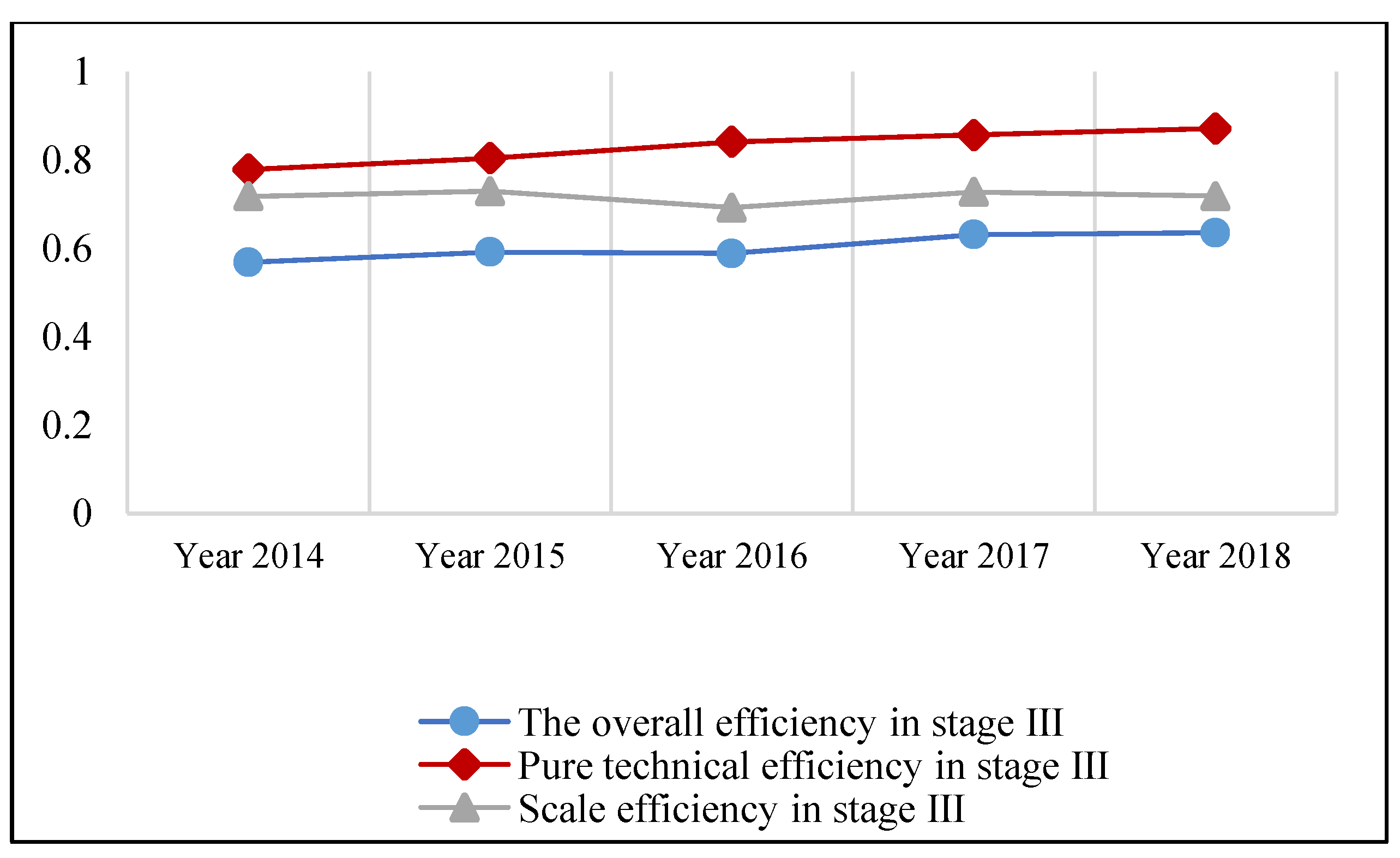
5.3. Stage III: Adjusted Efficiency Analysis

In stage III, the adjusted input was used as input, keeping the original output unchanged, and the DEA-BCC model was reused for operation. The results are shown in

Table 4. The efficiency value of China’s coastal ports in stage III (2014–2018).

Port	2014				2015				2016				2017				2018				Five-Year Average
	Crste	Vrste	Scale		Crste	Vrste	Scale		Crste	Vrste	Scale		Crste	Vrste	Scale		Crste	Vrste	Scale		Crste	Vrste	Scale
Dalian	0.526	0.534	0.985	drs	0.511	0.515	0.993	drs	0.589	0.594	0.993	irs	0.623	0.635	0.982	irs	0.64	0.651	0.983	irs	0.578	0.586	0.987
Qingdao	1	1	1	-	1	1	1	-	1	1	1	-	1	1	1	-	1	1	1	-	1	1	1
Rizhao	1	1	1	-	1	1	1	-	0.991	1	0.991	irs	0.942	1	0.942	irs	0.944	1	0.944	irs	0.975	1	0.975
Qinhuangdao	0.919	1	0.919	irs	0.671	0.819	0.819	irs	0.513	0.883	0.582	irs	0.713	0.959	0.744	irs	0.726	0.965	0.752	irs	0.708	0.925	0.763
Tianjin	0.758	1	0.758	drs	0.789	1	0.789	drs	0.79	0.907	0.871	drs	0.934	0.941	0.992	irs	1	1	1	-	0.854	0.97	0.882
Yantai	0.564	0.779	0.723	irs	0.618	0.829	0.746	irs	0.633	0.834	0.759	irs	0.493	0.582	0.846	irs	0.487	0.596	0.818	irs	0.559	0.724	0.778
Yingkou	0.801	0.834	0.96	irs	0.838	0.876	0.957	irs	0.856	0.914	0.937	irs	0.896	0.983	0.911	irs	0.911	1	0.911	irs	0.86	0.921	0.935
Lianyungang	0.582	1	0.582	irs	0.579	0.962	0.602	irs	0.587	1	0.587	irs	0.629	1	0.629	irs	0.617	1	0.617	irs	0.599	0.992	0.603
Ningbo-Zhoushan	0.502	1	0.502	drs	0.549	1	0.549	drs	0.586	1	0.586	drs	0.657	1	0.657	drs	0.648	1	0.648	drs	0.588	1	0.588
Shanghai	0.61	1	0.61	drs	0.704	1	0.704	drs	0.795	1	0.795	drs	0.854	1	0.854	drs	0.846	1	0.846	drs	0.762	1	0.762
Wenzhou	0.184	0.433	0.425	irs	0.488	0.688	0.709	irs	0.231	0.658	0.35	irs	0.265	0.705	0.376	irs	0.265	0.746	0.355	irs	0.287	0.646	0.443
Fuzhou	0.286	0.496	0.576	irs	0.268	0.477	0.562	irs	0.283	0.59	0.48	irs	0.307	0.571	0.537	irs	0.296	0.602	0.492	irs	0.288	0.547	0.529
Xiamen	0.416	0.541	0.768	irs	0.42	0.572	0.733	irs	0.43	0.597	0.72	irs	0.472	0.653	0.723	irs	0.478	0.669	0.715	irs	0.443	0.606	0.732
Guangzhou	0.486	0.517	0.941	drs	0.593	0.627	0.946	drs	0.653	0.714	0.914	drs	0.723	0.828	0.874	drs	0.737	0.848	0.87	drs	0.638	0.707	0.909
Shantou	0.218	0.742	0.294	irs	0.212	0.845	0.252	irs	0.201	0.977	0.205	irs	0.207	1	0.207	irs	0.206	1	0.206	irs	0.209	0.913	0.233
Shenzhen	0.95	1	0.95	drs	1	1	1	-	0.991	1	0.991	drs	1	1	1	-	1	1	1	-	0.988	1	0.988
Zhuhai	0.249	0.483	0.514	irs	0.27	0.535	0.505	irs	0.281	0.617	0.455	irs	0.339	0.632	0.537	irs	0.342	0.639	0.536	irs	0.296	0.581	0.509
Fangchenggang	0.314	0.576	0.545	irs	0.312	0.611	0.51	irs	0.298	0.73	0.408	irs	0.291	0.668	0.435	irs	0.297	0.726	0.409	irs	0.302	0.662	0.461
Haikou	0.506	1	0.506	irs	0.437	1	0.437	irs	0.41	1	0.41	irs	0.474	1	0.474	irs	0.473	1	0.473	irs	0.46	1	0.46
Zhanjiang	0.512	0.638	0.802	irs	0.585	0.74	0.791	irs	0.671	0.817	0.821	irs	0.821	0.981	0.837	irs	0.813	1	0.813	irs	0.68	0.835	0.813
Mean	0.569	0.779	0.718		0.592	0.805	0.73		0.589	0.842	0.693		0.632	0.857	0.728		0.636	0.872	0.719

Note: crste, comprehensive efficiency; vrste, pure technical efficiency; scale, scale efficiency; drs, diminishing returns to scale; irs, increasing returns to scale; -, constant returns to scale.

. Considering the influence of environmental factors and random errors, the results of this stage could have been different from those of the first stage. If the original low-efficiency port was improved after adjustment, the environment of the port was relatively poor. In the same way, a drop in efficiency indicates a relatively favorable environment.

(1) Efficiency comparison before and after adjustment

For the convenience of observation, the average comprehensive efficiency, pure technical efficiency, and scale efficiency of each port in the past five years were selected for comparison.

The difference between before and after adjustment was reflected by the average value of the comprehensive efficiency of each port from 2014 to 2018, as shown in Table 2 and Table 4. After adjustment, the comprehensive efficiency of most ports changed compared with the first stage, which means that environmental factors had an impact on the redundancy of various inputs. Compared with the first stage, the average comprehensive efficiency of 10 ports improved, that of 2 ports remained unchanged, and that of 8 ports decreased. Among them, Tianjin port showed the highest increase from 0.731 to 0.854, indicating that the external environment of the port was relatively poor and was underestimated in the first stage. The largest decline was for Haikou port, which dropped from 0.569 to 0.460, indicating that the port is located in a relatively friendly environment and its efficiency was overestimated.

As shown in Table 2 and Table 4, after the adjustment, the pure technical efficiency of each port did not decline, that of six ports remained unchanged, and that of the others improved. Among them, Yantai, Wenzhou, Fuzhou, Zhuhai, and Fangcheng significantly increased, all by more than 0.1. These results show that the technical environment and management level of these ports were relatively low. Compared with other ports, their production infrastructure and equipment still need to be improved.

As shown in Table 2 and Table 4, after adjustment, the scale efficiency of most ports declined, and only that of five ports improved: Dalian, Tianjin, Ningbo-Zhoushan, Shanghai, and Guangzhou ports. Fuzhou port showed the most obvious decline from 0.702 to 0.529. Yantai, Zhuhai, Fangcheng, and Haikou ports also showed obvious declines. For ports with increasing returns to scale, it is necessary to appropriately increase the investment in production facilities to expand the scale. For example, they should appropriately increase the number of berths, widen the length of the production wharf, and construct 10,000-ton berths. Ports with diminishing returns to scale mainly need to improve their technology and management level rather than excessively pursue scale expansion.

(2) Logistics efficiency trend of China’s coastal ports from 2014 to 2018

As shown in Figure 1, from the perspective of time, after excluding environmental differences and random errors, the pure technical efficiency from 2014 to 2018 increased year by year while the scale efficiency remained at around 0.7. These results indicate that China’s coastal ports improved the operation capacity of production infrastructure, as well as that the technical level and management environment also improved in recent years. The scale efficiency was not as high as the pure technical efficiency in each year, which reflects the phenomena of blind expansion of scale and waste of resources in most of China’s coastal ports. The improvement of overall efficiency was mainly due to pure technical efficiency. It is not difficult to see that scale efficiency largely has hindered the improvement of overall efficiency. These results show that China’s coastal ports unilaterally pursued cargo and container throughput and invested too much in infrastructure construction, resulting in idle berths and a large number of berths not being reasonably utilized.

(3) Comparison of logistics efficiency of coastal ports in various regions

China’s coastal ports have regional characteristics. The coastal ports were divided into five port clusters by the Ministry of Communications in September 2006, as shown in

Table 5. The five major regional divisions.

Region	Port
Bohai Rim port cluster	Dalian Port, Qingdao Port, Rizhao Port, Qinhuangdao Port, Tianjin Port, Yantai Port, Yingkou Port
Yangtze River Delta coastal port cluster	Lianyungang Port, Ningbo-Zhoushan Port, Shanghai Port, Wenzhou Port
Southeast coastal port cluster	Fuzhou Port, Xiamen Port
Pearl River Delta port cluster	Guangzhou Port, Shantou Port, Shenzhen Port, Zhuhai Port
Southwest coastal port cluster	Fangchenggang Port, Haikou Port, Zhanjiang Port

. Based on this, the difference in logistics efficiency of coastal ports was explored.

As shown in

Table 6. The average value of port logistics efficiency by region (2014-2018).

Region	Stage I			Stage III
	Crste	Vrste	Scale	Crste	Vrste	Scale
Bohai Rim port cluster	0.759	0.825	0.924	0.791	0.875	0.903
Yangtze River Delta coastal port cluster	0.527	0.873	0.592	0.559	0.910	0.599
Southeast coastal port cluster	0.366	0.479	0.754	0.366	0.577	0.631
Pearl River Delta port cluster	0.528	0.740	0.705	0.533	0.800	0.660
Southwest coastal port cluster	0.516	0.772	0.667	0.481	0.832	0.578
Mean	0.539	0.738	0.728	0.546	0.799	0.674

, from a regional perspective, the comprehensive efficiency of ports around the Bohai Rim, Yangtze River Delta, and Pearl River Delta port clusters improved after adjustment, though the improvement was not large. The Bohai Rim port cluster still had the highest comprehensive efficiency (0.791), and the Southeast coastal port cluster ranked last with a comprehensive efficiency value of 0.366.

These results show that the overall efficiency of port logistics in China from 2014 to 2018 was at a low level. In terms of pure technical efficiency, all regions performed relatively well. Although the Yangtze River Delta coastal port cluster ranked first in pure technical efficiency (0.910), the scale efficiency was only 0.599. The Pearl River Delta and Southwest coastal port clusters also showed relatively low overall efficiency due to a low scale efficiency.

Based on the above analysis, our recommendations are as follows. For regional ports with a low overall efficiency due to a low scale efficiency, the input of various production factors should be strictly controlled (while maintaining a sustainable port management environment and technical level), especially the construction of port infrastructure, and the scale should be appropriately expanded according to actual development. For regional ports with a low pure technical efficiency and a low scale efficiency, it is necessary to not only improve the port management system and the level of production technology but also to strengthen the integration of port resources, reduce investment redundancy, and improve efficiency.

(4) Cluster analysis of coastal port logistics efficiency

The matrix in Figure 2 reflects the market competitiveness of China’s coastal ports from the perspective of efficiency and output, and it makes it easy to understand the advantages and disadvantages of various ports. In the matrix, the average comprehensive efficiency of all ports (0.604) is on the horizontal axis and the average throughput of all ports (320.49 million tons) is on the vertical axis. The matrix was used for the cluster analysis of coastal port logistics efficiency.

(1) “Abundant” port

This type of port performs better in throughput and efficiency. Usually, it has great advantages in terms of cargo source, economic environment, and collection and distribution systems. For example, Qingdao, Rizhao, Yingkou, and Tianjin ports in the Bohai Rim region have good geographical locations. The coastline of the region is nearly 5700 km long, accounting for about one-third of the country’s coastline. It is regarded as the main gate of China’s shipping market. According to its advantages, it should reasonably allocate port resources, appropriately reduce the number of berths, integrate berths with a short distance, and promote the construction of 10,000-ton and 100,000-ton berths while maintaining a steady increase in output. In addition, investment in intelligent technology should be strengthened to improve the level of port information.

(2) “Refined” port

This type of port performs better in efficiency, but its throughput output is relatively weak. In general, such ports can reasonably invest and allocate port resources to improve efficiency. However, due to their awkward location and relatively few sources of goods, these ports should cooperate with other ports in the region to promote increased trade volume so as to ensure the source of goods.

(3) “Fat” port

This type of port has a relatively large advantage in throughput, but its efficiency is relatively low. Such ports are usually large in scale, but they do not have a good grasp of infrastructure investment and resource allocation. Generally, the construction of berths requires a large amount of capital investment and a long recovery period, and the investment in infrastructure is irreversible. For this type of port, the internal planning of the port and the rational distribution of production factors should be the focus of work.

(4) “Lean” port

This type of port has low levels of efficiency and throughput. Such ports may be in a poor state in both respects due to their small scale, unreasonable investment in infrastructure, limited economic level in the hinterland, and inadequate external collection and distribution systems. In this regard, these ports should first improve their internal management capability and effectively integrate resources to ensure business capability. Second, they should strengthen cooperation with neighboring ports to ensure that a certain amount of trade is maintained. Finally, hinterland cities should improve their economic levels in both quality and quantity, as well as strengthen the construction of inland transportation infrastructure, in order to provide a sustainable external environment for the port to improve its efficiency and therefore transform into a refined port.

5.4. Stage IV: Analysis of Influencing Factors Based on Tobit Model

Stage II analysis verified that environmental variables can have an impact on input redundancy, but the same environmental variable can have different effects on each instance of input redundancy in many cases. Therefore, the influence direction of a particular environmental factor on port logistics efficiency cannot be determined. Based on these results and considering the comprehensive efficiency of stage III as the dependent variable and the environmental factors as the independent variables, the Tobit model was used to explore the degree and direction of the impact of various environmental factors on port logistics efficiency. Comparing the evaluation mode from the literature [33], the four-stage DEA was used to identify explicit causes of inefficiency based on more scientific evidence.

The external environmental variables under investigation were divided into economic level and transportation conditions. The economic level was set to include GDP, foreign trade level, and scale of service industry in hinterland cities. The level of transportation condition was set to include road network construction and public service capacity in hinterland cities. The results are shown in

Table 7. The results of factors influencing logistics efficiency of China’s coastal ports.

	Coefficient	Standard Deviation	Z Value	p Value
Economic level	0.0000279	6.04 × 10−6	4.02	0.000 ***
Foreign trade level	−0.0000806	0.0000423	−1.78	0.075 *
Scale of service industry	−0.0000302	0.0000129	−2.34	0.019 **
Road network construction	0.0139583	0.0045271	2.99	0.003 ***
Public service capacity	0.0000182	9.30 × 10−6	1.96	0.05 **
Constant	0.3894028	0.0758252	5.14	0.000 ***

Note: *, **, ***, respectively indicate significance at 90%, 95%, 99% confidence level.

.

The GDP of port hinterland cities was found to be positively correlated with port logistics efficiency, and it was significant at the 99% confidence level. This indicates that the rapid economic growth of port hinterland cities promotes the improvement of port logistics efficiency over a certain period of time. With improved economic strength, hinterland cities can increase their investment in constructing port production infrastructure, which would also bring a relatively considerable output of cargo throughput and thereby improve the efficiency of port logistics.

Foreign trade level was found to be negatively correlated with port logistics efficiency, which was significant at the 95% confidence level. An improved foreign trade level is attributable to increased total import and export volume. However, if a large amount of infrastructure construction cost is sacrificed as a condition for increasing the foreign trade level, the improvement of port logistics efficiency would be restricted. For inefficient ports, this also shows that hinterland cities do not invest in infrastructure construction due to the one-sided pursuit of improving the foreign trade level, resulting in a failure to improve port logistics efficiency.

The scale of the service industry was found to be negatively correlated with port logistics efficiency, which was significant at the 95% confidence level. This means that it is not appropriate to increase investment in the scale of the service industry for ports with a low logistics efficiency because of the characteristics of the long construction and payback periods of port production infrastructure—especially the construction of berths, for which its usually take more than five years to recover the cost, thus resulting in increased investment but no output.

Road network construction and public service capacity in port hinterland cities were found to be positively correlated with port logistics efficiency and were significant at the 95% confidence level, which indicates that they play a positive role in improving logistics efficiency. Since it is difficult to expand an urban administrative area in a short period of time, for ports with a low logistics efficiency, hinterland cities should reasonably plan an inland transportation system. They can improve the efficiency of port logistics by implementing measures such as strengthening highway construction, increasing the mileage of highways to increase the density of the highway network, and increasing investment in public buses (electric vehicles). These results also show that improving the efficiency of port logistics should not only rely on improving internal production technology, facilities, and equipment but also pay attention to the external traffic conditions of the port and the capability of the collection and distribution system.

6. Conclusion and Suggestions

Logistics is one of the fastest growing sectors in the world, and its efficiency evaluation is considered to be a key competency to acquire world-class efficiency [24]. Since the port production mode itself has the characteristics of logistics function, we selected 20 main coastal ports in China as the research object in this study. The logistics efficiency of China’s coastal ports was systematically evaluated with four-stage DEA including the Tobit model. Specifically, the logistics efficiency of coastal ports was accurately measured, the market competitiveness characteristic of China’s coastal ports was clearly analyzed, and the path for improving logistics efficiency was explored. Several conclusions can be drawn from the empirical evidence as follows:

(1)

The pure technical efficiency of most ports was underestimated and the scale efficiency was overestimated in the first stage. After adjusting the external environment in the second stage, the logistics efficiency of most of China’s coastal ports was in a low state from 2014 to 2018. The reason for the low efficiency is that the scale efficiency had not been improved. Judging from the change trend from 2014 to 2018, the overall logistics efficiency of coastal ports is on the rise. During this period, only the Qingdao, Rizhao, and Shenzhen ports performed well, maintaining a comprehensive efficiency value of over 0.9 every year. The strengths of each port in each region showed that the ports around the Bohai Sea have a relatively good overall performance and the ports along the Yangtze River Delta have a higher pure technical efficiency. It was also found that the impact of environmental variables on input redundancy varies from year to year.

(2)

By applying the Tobit model, we found that the impact degree and direction of different environmental variables on port logistics efficiency were different. During the study period, the increased road network construction and GDP in port hinterland cities promoted the improvement of port logistics efficiency. The foreign trade level was found to have an inhibitory effect on the improvement of port logistics efficiency. An increased scale of the service industry in hinterland cities was not shown to be conducive to improving the efficiency of port logistics.

Based on the conclusions described above, the following suggestions are put forward to improve the logistics efficiency of China’s coastal ports:

(1)

Promote the coordinated development of port logistics and hinterland cities. Hinterland cities should ensure a steady improvement in quality while increasing the GDP level. As port cities, their key economic development targets should be their ports. Local governments should provide targeted policy support and financial assistance according to the actual operating conditions of each port so that improving the economic level can become a booster for improving the port logistics efficiency.

(2)

Enable reasonable planning and key construction. The development direction of ports that emphasizes scale and light planning should be avoided as much as possible. In addition, ports with a low scale efficiency should strengthen their resource integration in order to improve resource waste. For those low-competitive ports, it is difficult for the proportion of increased output to be equal to the proportion of increased input, so it is difficult to improve the scale efficiency. In this regard, regions should cooperate and each port should seek business differentiation to reduce the degree of such competition.

(3)

Strengthen foreign trade and attract supply. Against the background of the 21st Century Maritime Silk Road, Chinese coastal ports should strengthen trade and exchanges with countries along the route to attract investment from foreign-funded enterprises. At the same time, they should also actively link with ports of countries along the route to form a sustainable maritime transportation network to achieve mutual benefit with neighboring countries.

(4)

Build and improve the collection and distribution system of hinterland cities, as well as promote the development of port logistics. Coastal ports have become important nodes of the integrated logistics chain. Improving the inland transportation system will help to ensure the safety of cargo transportation and improve the speed of cargo concentration in ports. Hinterland cities should rationally plan the construction of highways, appropriately increase the mileage of highways, improve the external collection and distribution system of ports, improve the speed of goods collection and distribution in ports, and increase the output of ports.

(5)

Introduce new technologies to realize smart ports. Chinese coastal ports should speed up the application of new technologies in port logistics. In terms of software facilities, port enterprises should promote the application of new information technologies such as 5G, the BeiDou positioning and navigation system, cloud computing, big data, and sensors as soon as possible to improve the information level of ports. In terms of hardware facilities, loading and unloading equipment and dispatching and transshipment equipment should be upgraded with the aim of reaching international standards. A combination of software and hardware is also necessary.

For the variables needed to evaluate the efficiency of port logistics, the difficulty of obtaining relevant data is inconsistent. Thus, the input variable only adopts the number and length of berths. In future research, more input variables (including the number of port employees and port construction investment) should be selected to enable the more accurate calculation of port logistics efficiency. An additional limitation in this study was that other coastal ports were not considered.

References

1. Wu, Y.C.J.; Goh, M. Container port efficiency in emerging and more advanced markets. Transp. Res. Part E 2010, 46, 1030–1042. [Google Scholar] [CrossRef]
2. Guner, S. Incorporating value judgments into port efficiency measurement models: From Turkish ports. Marit. Econ. Logist. 2018, 20, 569–586. [Google Scholar] [CrossRef]
3. Cao, L.L. Changing port governance model: Port spatial structure and trade efficiency. J. Coastal Res. 2020, 95, 963–968. [Google Scholar] [CrossRef]
4. Hatami-Marbini, A.; Saati, S.; Tavana, M. An ideal-seeking fuzzy data envelopment analysis framework. Appl. Soft Comput. 2010, 10, 1062–1070. [Google Scholar] [CrossRef]
5. Sav, G.T. Four-Stage DEA Efficiency Evaluations: Financial Reforms in Public University Funding. Int. J. Econ. Financ. 2012, 5, 24–33. [Google Scholar] [CrossRef]
6. Zeng, S.; Jiang, C.; Ma, C.; Su, B. Investment efficiency of the new energy industry in China. Energy Econ. 2018, 70, 536–544. [Google Scholar] [CrossRef]
7. Hu, J.L.; Lio, M.C.; Yeh, F.Y.; Lin, C.H. Environment-adjusted regional energy efficiency in Taiwan. Appl. Energy 2011, 88, 2893–2899. [Google Scholar] [CrossRef]
8. Lu, S.; Li, S.; Zhou, W. Does government subsidy stimulate or shackle new energy industry efficiency? Evidence from China. Environ. Sci. Pollut. Res. 2022, 29, 34776–34797. [Google Scholar] [CrossRef]
9. Wang, F.C.; Hung, W.T.; Shang, J.K. Measuring pure managerial efficiency of international tourist hotels in Taiwan. Serv. Ind. J. 2006, 26, 59–71. [Google Scholar] [CrossRef]
10. Lado-Sestayo, R.; Fernández-Castro, Á.S. The impact of tourist destination on hotel efficiency: A data envelopment analysis approach. Eur. J. Oper. Res. 2019, 272, 674–686. [Google Scholar] [CrossRef]
11. Medina-Borja, A.; Triantis, K. Modeling social services performance: A four-stage DEA approach to evaluate fundraising efficiency, capacity building, service quality, and effectiveness in the nonprofit sector. Ann. Oper. Res. 2014, 221, 285–307. [Google Scholar] [CrossRef]
12. Goyal, G.; Dutta, P. Performance analysis of Indian states based on social–economic infrastructural investments using data envelopment analysis. Int. J. Product. Perform. Manag. 2021, 70, 2258–2280. [Google Scholar] [CrossRef]
13. Zheng, W.; Sun, H.; Zhang, P.; Zhou, G.; Jin, Q.; Lu, X. A four-stage DEA-based efficiency evaluation of public hospitals in China after the implementation of new medical reforms. PLoS ONE 2018, 13, e0203780. [Google Scholar] [CrossRef]
14. Shieh, H.S.; Hu, J.L.; Ang, Y.Z. Efficiency of Life Insurance Companies: An Empirical Study in Mainland China and Taiwan. SAGE Open 2020, 10, 1–17. [Google Scholar] [CrossRef]
15. Clark, E.; Qiao, Z. The post-SOX comparative dynamics of public accounting firm efficiency. Account. Res. J. 2022, 35, 178–195. [Google Scholar] [CrossRef]
16. Tsaur, R.C.; Chen, I.F.; Chan, Y.S. TFT-LCD industry performance analysis and evaluation using GRA and DEA models. Int. J. Prod. Res. 2016, 55, 4378–4391. [Google Scholar] [CrossRef]
17. Li, H.; Zhu, X.; Chen, J. Total factor waste gas treatment efficiency of China’s iron and steel enterprises and its influencing factors: An empirical analysis based on the four-stage SBM-DEA model. Ecol. Indic. 2020, 119, 106812. [Google Scholar] [CrossRef]
18. Chen, Y.; Cheng, S.; Zhu, Z. Measuring environmental-adjusted dynamic energy efficiency of China’s transportation sector: A four-stage NDDF-DEA approach. Energy Effic. 2021, 14, 35. [Google Scholar] [CrossRef]
19. Fugate, B.S.; Mentzer, J.T.; Stank, T.P. Logistics performance: Efficiency, effectiveness, and differentiation. J. Bus. Logist. 2010, 31, 43–62. [Google Scholar] [CrossRef]
20. Tongzon, J.; Heng, W. Port privatization, efficiency and competitiveness: Some empirical evidence from container ports (terminals). Transp. Res. Part A: Policy Pract. 2005, 39, 405–424. [Google Scholar] [CrossRef]
21. Dai, J. Evaluation Method of Logistics Transportation Efficiency of Port Enterprises Based on Game Model. J. Coast. Res. 2020, 103 (Supp. 1), 609–613. [Google Scholar] [CrossRef]
22. Zheng, W.; Xu, X.; Wang, H. Regional logistics efficiency and performance in China along the Belt and Road Initiative: The analysis of integrated DEA and hierarchical regression with carbon constraint. J. Clean. Prod. 2020, 276, 123649. [Google Scholar] [CrossRef]
23. Nguyen, N.T.; Tran, T.T. Raising opportunities in strategic alliance by evaluating efficiency of logistics companies in Vietnam: A case of Cat Lai Port. Neural Comput. Appl. 2019, 31, 7963–7974. [Google Scholar] [CrossRef]
24. Çakır, S. Measuring logistics performance of OECD countries via fuzzy linear regression. J. Multi-Criteria Decision Anal. 2017, 24, 177–186. [Google Scholar] [CrossRef]
25. Hamdan, A.; Rogers, K.J. Evaluating the efficiency of 3PL logistics operations. Int. J. Prod. Econ. 2008, 113, 235–244. [Google Scholar] [CrossRef]
26. Zhang, H.; You, J.; Haiyirete, X.; Zhang, T. Measuring Logistics Efficiency in China Considering Technology Heterogeneity and Carbon Emission through a Meta-Frontier Model. Sustainability 2020, 12, 8157. [Google Scholar] [CrossRef]
27. Schøyen, H.; Bjorbæk, C.T.; Steger-Jensen, K.; Bouhmala, N.; Burki, U.; Jensen, T.E.; Berg, Ø. Measuring the contribution of logistics service delivery performance outcomes and deep-sea container liner connectivity on port efficiency. Res. Transp. Bus. Manag. 2018, 28, 66–76. [Google Scholar] [CrossRef]
28. Bajec, P.; Kontelj, M.; Groznik, A. Assessment oF logistics platForm efficiency using an integrated delphi analytic hierarchy process-data envelopment analysis approach: A novel methodological approach including a case study in slovenia. EM Ekon. A Manag. 2020, 23, 191–207. [Google Scholar] [CrossRef]
29. Cullinane, K.; Wang, T.F.; Song, D.W.; Ji, P. The technical efficiency of container ports: Comparing data envelopment analysis and stochastic frontier analysis. Transp. Res. Part A: Policy Pract. 2006, 40, 354–374. [Google Scholar] [CrossRef]
30. Mustafa, F.S.; Khan, R.U.; Mustafa, T. Technical efficiency comparison of container ports in Asian and Middle East region using DEA. Asian J. Shipp. Logist. 2021, 37, 12–19. [Google Scholar] [CrossRef]
31. Charnes, A.T.; Cooper, W.W. Efficiency characterizations in different DEA models. Socio-Econ. Plan. Sci. 1988, 22, 253–257. [Google Scholar] [CrossRef]
32. Fried, H.O.; Lovell, C.A.K.; Schmidt, S.S.; Yaisawarng, S. Accounting for environmental effects and statistical noise in data envelopment analysis. J. Product. Anal. 2002, 17, 157–174. [Google Scholar] [CrossRef]
33. Cruz, M.R.P.; Ferreira, J.J.M. Evaluating lberian seaport competitiveness using an alternative DEA approach. Eur. Transp. Res. Rev. 2016, 8, 1. [Google Scholar] [CrossRef]
34. Gan, W.H.; Yao, W.P.; Huang, S.Y. Evaluation of green logistics efficiency in Jiangxi province based on three-stage DEA from the perspective of high-quality development. Sustainability 2022, 14, 797. [Google Scholar] [CrossRef]
35. Wu, Y.C.J.; Lin, C.W. National port competitivveness: Implications for India. Manag. Decis. 2008, 46, 1482–1507. [Google Scholar] [CrossRef]
36. Song, Y.W.; Liu, H.G. Internet development, economic level, and port total factor productivity: An empirical study of yangtze river ports. Int. J. Logist. Res. Appl. 2019, 23, 375–389. [Google Scholar] [CrossRef]
37. Dias, J.C.Q.; Azevedo, S.G.; Ferreira, J.; Palma, S.F. A comparative benchmarking analysis of main lberian container terminals: A DEA approach. Int. J. Shipp. Transp. Logist. 2009, 3, 260–275. [Google Scholar] [CrossRef]
38. Wanke, P.; Barros, C.P. New evidence on the determinants of efficency at Brazilian ports: A bootstraped DEA analysis. Int. J. Shing Transp. Logist. 2016, 8, 250–272. [Google Scholar] [CrossRef]
Figure 1. The average efficiency of China’s major coastal ports (2014–2018).
Jmse 10 01147 g001
Figure 2. The port logistics efficiency throughput matrix.
Jmse 10 01147 g002